Solving a reverse supply chain design problem by improved Benders decomposition schemes

(1)

Solving a reverse supply chain design problem by improved Benders

decomposition schemes

q

Ernesto D.R. Santibanez-Gonzalez

a,⇑

_{, Ali Diabat}

b a_{Departamento de Computação, Universidade Federal de Ouro Preto, Ouro Preto, MG, Brazil}

b_{Department of Engineering Systems & Management, Masdar Institute of Science & Technology, Abu Dhabi, UAE}

a r t i c l e

i n f o

Article history: Received 3 October 2012

Received in revised form 11 May 2013 Accepted 6 September 2013 Available online 18 September 2013

Keywords:

Supply chain management Reverse logistics Benders decomposition Mixed-integer programming

a b s t r a c t

In this paper we propose improved Benders decomposition schemes for solving a remanufacturing supply chain design problem (RSCP). We introduce a set of valid inequalities in order to improve the quality of the lower bound and also to accelerate the convergence of the classical Benders algorithm. We also derive quasi Pareto-optimal cuts for improving convergence and propose a Benders decomposition scheme to solve ourRSCPproblem. Computational experiments for randomly generated networks of up to 700 sourcing sites, 100 candidate sites for locating reprocessing facilities, and 50 reclamation facilities are presented. In general, according to our computational results, the Benders decomposition scheme based on the quasi Pareto-optimal cuts outperforms the classical algorithm with valid inequalities.

1. Introduction

Adopting a friendly sustainable management approach implies a number of changes for companies from the strategic level up to the operational point of view, affecting their employees and impacting their business processes and technology. In this regard,

Simchi-Levi, Kaminsky, and Simchi-Levi (2007) point out, ‘‘the strategic level deals with decisions that have a long-lasting effect on the firm. These include decisions regarding the number, loca-tion and capacities of warehouses and manufacturing plants, or the flow of material through the logistics network.’’

The problem of locating facilities and allocating customers is not new to the operations research community and involves the key aspects of supply chain design (Daskin, Snyder, & Berger, 2005). This problem is one of ‘‘the most comprehensive strategic decision problems that need to be optimized for long-term effi-cient operation of the whole supply chain’’ (Altiparmak, Gen, Lin, & Paksoy, 2006). As observed byFarahani and Hekmatfar (2009), some small changes to classical facility location models can make the problems much harder to solve.

In the last few years, mathematical modeling and solution methods for the efficient management of return flows (and/or inte-grated with forward flows) have been studied in the context of re-verse logistics, closed-loop supply chains, and sustainable supply chains.

Fleischmann, Krikke, Dekker, and Flapper (2000)discussed new issues that arise in the context of reverse logistics, and they reviewed the mathematical models proposed in the literature.

Fleischmann, Beullens, Bloemhof-Ruwaard, and Va (2001) pro-posed a generic recovery network model based on the elementary characteristics of return networks identified inFleischmann et al. (2000).Zhou and Wang (2008)proposed a generic mixed integer model for the design of a reverse distribution network including repairing and remanufacturing options simultaneously.

Regarding reverse logistics networks in connection with loca-tion problems,Bloemhof-Ruwaard, Salomon, and Van Wassenhove (1996)presented a two-level distribution and waste disposal prob-lem, in which demand for products is met by plants while the waste generated by production is correctly disposed of at waste disposal units.Barros, Dekker, and Scholten (1998)described a net-work for recycling sand from construction waste and proposed a two-level location model to solve the location problem of two types of intermediate facilities.

Regarding remanufacturing location models, Krikke, Van Harten, and Schuur (1999)described a small reverse logistics net-work for the returns, processing, and recovery of discarded copiers. They presented a mixed integer linear programming (MILP) model based on a multi-level uncapacitated warehouse location model. The model was used to determine the locations and capacities of the recovery facilities as well as the transportation links connect-ing various locations. In Jayaraman, Patterson, and Rolland (2003), a 0–1 MILP model for a product recall distribution problem is proposed. They analyzed a particular case in which the customer returns the product to a retail store, and the product is sent to a

q

The manuscript was processed by the area editor Qiuhong Zhao.

⇑ Corresponding author. Tel.: +55 31 3559 1692.

E-mail address:santibanez@iceb.ufop.br(E.D.R. Santibanez-Gonzalez).

Contents lists available atScienceDirect

Computers & Industrial Engineering

(2)

refurbishing site which will rework the product or properly dis-pose it. The reverse supply chain is comdis-posed of origination, collec-tion, and refurbishing sites. With the objective to minimize fixed and distribution costs, the model has to decide which collection sites and which refurbishing sites to open, subject to a limit on the number of collection sites and refurbishing sites that can be opened.

Several authors have studied different aspects of closed-loop supply chain problems. See, for example,Jayaraman, Guide, and Srivastava (1999), Fleischmann (2003), Barbosa-Povoa, Salema, and Novais (2007), Guide and Van Wassenhove (2009) and Neto, Walther, Bloemhof-Ruwaard, Van Nunen, and Spengler (2010). Sahyouni, Savaskan, and Daskin (2007) presented three generic facility location MIP models for integrated decision making in the design of forward and reverse logistics networks. The formulations are based on the well-known uncapacitated fixed-charge location model, and they include the location of used product collection centers and the assignment of product return flows to these cen-ters.Lu and Bostel (2007)presented a two-level location problem with three types of facilities to be located in a reverse logistics sys-tem. They proposed a 0–1 MILP model which simultaneously con-siders ‘‘forward’’ and ‘‘reverse’’ flows and their mutual interactions. The model has to decide the number and locations of three differ-ent types of facilities: producers, remanufacturing cdiffer-enters, and intermediate centers.

In summary, reverse logistics models are chronologically dis-cussed by Bloemhof-Ruwaard et al. (1996), Barros et al. (1998), Krikke et al. (1999), Fleischmann et al. (2000, 2001), Shih (2001), Sodhi and Reimer (2001), Jayaraman et al. (2003), Le Blanc, Fleuren, and Krikke (2004), Listesßand Dekker (2005), and more recently

Zhou and Wang (2008), Salema, Barbosa-Povoa, and Novais (2010), Gomes, Barbosa-Povoa, and Novais (2011) and Alumur, Nickel, Saldanha-da-Gama, and Verter (2012). Almost all of this re-search proposed MILP models. Listesßand Dekker proposed a sto-chastic MILP and Alumur et al. studied the dynamic factors that affect location decisions. The majority of solution methods are based on standard commercial packages.

In this paper, the problem of designing a reverse supply chain network is addressed, and a Benders decomposition-based algo-rithm is proposed for solving it. The problem is a NP-hard combi-natorial optimization problem. The MILP model follows some previously published work by, for example, Jayaraman et al. (2003), Salema et al. (2010) and Li (2011), but in this paper we de-velop a more efficient algorithm for solving it. For randomly gener-ated test instances of the problem, we analyze the performance of the algorithms in term of computational times and quality of the solution obtained.

This paper makes three primary contributions. First, it proposes a Benders decomposition algorithm for solving large-scale reverse network design problems. We test two sets of valid inequalities to strengthen the Relaxed Master Problem in order to improve the quality of the lower bound. Second, we derive quasi Pareto-optimal cuts as another strategy to accelerate convergence, and third, we propose a primal based Benders decomposition algorithm for solv-ing the problem. Computational results are conducted on large-scale networks of up to 700 sourcing facilities, 100 candidate sites for locating reprocessing facilities, and 50 reclamation facilities (70010050). To the best of our knowledge, for this kind of problems, these are the largest problems explored and solved so far.

The remainder of this paper is organized as follows. In the sec-ond section, we formulate the mathematical model for the prob-lem. In the third section, the Benders decomposition-based algorithms for solving the problem are proposed. In the fourth sec-tion, we present some strategies for accelerating the convergence of the Benders algorithms. In the fifth section, the computational

experiments performed with the algorithms are presented. The last section contains our conclusions.

2. Model for designing a reverse supply chain network

The problem can be categorized as a single product, static, three-echelon, capacitated location model with known demand. The reverse supply chain network consists of three types of mem-bers: sourcing facilities (origination sites like a retail store), collec-tion sites, and reclamacollec-tion facilities. At the customer levels, there are product demands and used products ready to be recovered (for example, cell phones). We suppose that customers return products to origination sites like a retail store. At the second layer of the supply chain network, there are reprocessing centers (collec-tion sites) used only in the reverse channel, and they are responsi-ble for activities such as cleaning, disassembly, checking, and sorting, before the returned products are sent back to reclamation facilities. At the third layer, reclamation facilities accept the checked returns from intermediate facilities and they are responsi-ble for the process of reclamation. In this paper, we address the backward flow of returns coming from sourcing facilities and going to reclamation facilities through reprocessing facilities properly lo-cated at pre-defined sites. In such a supply chain network, the ‘‘re-verse’’ flow moves from customers through collection sites to reclamation facilities and is formed by used products. On the other hand, the ‘‘forward’’ flow moves from reclamation facilities directly to new products at points of sale.

2.1. RSCP model

In this model, it is assumed that new product demands and available quantities of used products are known and determinis-tic. All returned (used) products are first shipped back to collec-tion facilities where some of them will be discarded for various reasons, including poor quality. The checked return-products will then be sent back to reclamation facilities, where some of them may still be discarded. We introduce the following inputs and sets:

I the set of sourcing facilities at the first layer, indexed byi J the set of reclamation nodes at the third layer indexed by

j

K the set of candidate reprocessing facility locations at the mid layer, indexed byk

ai supply quantity at source locationi2I bj demand quantity at reclamation locationj2J

fk fixed cost of locating a mid layer reprocessing facility at

candidate sitek2K

gk management cost at a mid layer reprocessing facility at

candidate sitek2K

cik is the unit cost of delivering products atk2Kfrom a

source facility located ini2I

dkj is the unit cost of supplying demandj2Jfrom a mid layer

facility located ink2K

mk capacity at reprocessing facility locationk2K

We consider the following decision variables:

wk 1 if we locate a reprocessing facility at candidate site k2K, 0 otherwise

xik flow from source facilityi2Ito reprocessing facility

located atk2K

ykj flow from reprocessing facility located atk2Kto facility j2J

(3)

Minimize X k2K

fkwkþ X

i2I X

k2K

ðcikþgkÞxikþ X

k2K X

j2J

dkjykj ð1Þ

X

i2I

xik6mkwk

8

k2K ð2Þ

X

k2K

xik6ai

8

i2I ð3Þ

X

k2K

ykjPbj

8

j2J ð4Þ

X

i2I

xik¼ X

jJ

ykj

8

k2K ð5Þ

xik;ykjP0;

8

i2I;

8

j2J;

8

k2K ð6Þ

wk2 f0;1g

8

k2K ð7Þ

The objective function(1) minimizes the sum of the installation reprocessing facility costs plus management costs at the reprocess-ing facilities plus delivery costs from sourcreprocess-ing facilities to repro-cessing facilities and from these to reclamation facilities. Constraints(2)ensure that all of the products that arrive at repro-cessing sitek2Kmust be less than its capacity and that this facility must be opened. Constraints(3)guarantee that up to a volume ofai

return products available atiare going backward to facilityk2K. Constraints(4)warrant that the demand at facilityj2Jmust be sat-isfied by reprocessing facilities. Constraints(5)ensure that all the return products arriving to facilitykare also delivered to reclama-tion facilities. Constraints (6) are the standard nonnegative con-straints. Constraints(7) are the standard binary constraints. This model has O(n2) continuous variables where n=max{|I|, |J|, |K|} and |K| are binary variables. The number of constraints isO(n).

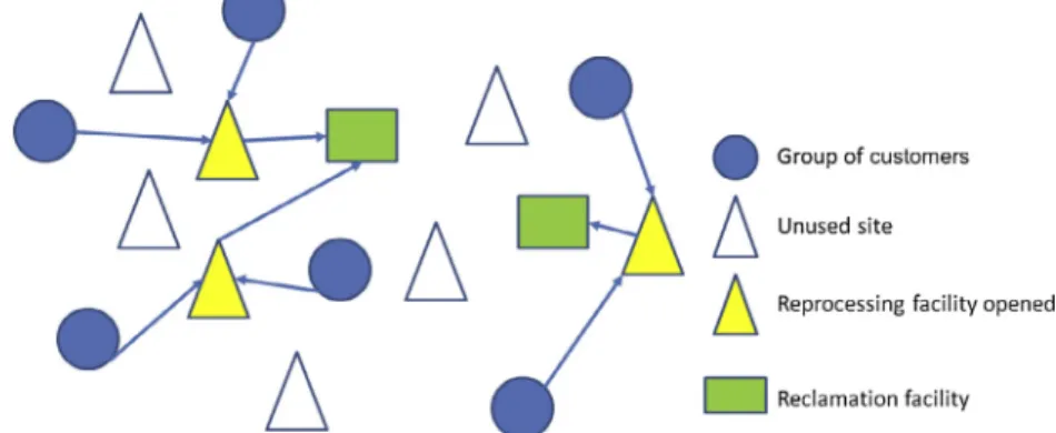
Fig. 1 shows a reverse supply chain network consisting of 6 groups of customers, 8 candidate sites for locating reprocessing facilities (with three facilities opened), and two reclamation facilities.

3. Benders decomposition

Benders decomposition is a classical decomposition technique (Benders, 1962) which is advisable for solving hard mixed integer programming problems with integer variables and coupling con-straints. Benders decomposition technique involves decomposing the overall formulation into a Master problem and a (Benders) sub-problem, and then solving them iteratively by utilizing the solution of one in the other. The Benders Master problem with only integer variables and an auxiliary variable is a relaxation of the primary problem. The auxiliary variable is introduced to facilitate the inter-action between the Master problem and the subproblem. In a min-imization problem, an optimal solution of the Benders Master problem provides a lower bound on the original problem and the values of the integer variables are passed through the subproblem for solving a new subproblem. By fixing the integer variables, the

primary problem with only continuous variables becomes a Bend-ers subproblem that can be solved easily. By solving the subprob-lem, the values of its dual variables and a valid upper bound for the primary problem (in the case of minimization) are obtained, and, in this case, by utilizing its objective value along with the cost com-ponents implied by the Master problem solution. The bounds are updated, and if the stopping criterion is not met, a Benders cut using the dual subproblem solution is generated. This new cut is appended to the Master problem, and the Benders decomposition algorithm is iterated continuously until a stopping criterion is met. To establish a stopping criteria, we employ a small percentage gap between the best upper and lower bounds and a maximum number of Benders cycles reached; whatever is achieved first ends the algorithm.

There are a number of publications to support the fact that the Benders algorithm has not been uniformly successful in all applica-tions; it has some deficiencies.Geoffrion and Graves (1974), among others, have noted that reformulating a mixed integer program can have a profound effect upon the efficiency of the algorithm. For the particular case of a network design problem (Magnanti & Wong, 1981), it has been observed that a straightforward implementation of the Benders algorithm often converged very slowly, requiring the solution of a large number of Relaxed Master Problems. The main issues associated with slow convergence of Benders algo-rithms are (a) the solution of Relaxed Master Problems and Bend-ers subproblems, and (b) the quality of the cuts produced in each iteration. To overcome these issues, accelerating techniques have been studied by a number of authors, among them: McDaniel and Devine (1977), Magnanti and Wong (1981), Côté and Laughton (1984), Papadakos (2008), Rei, Cordeau, Gendreau, and Soriano (2008), Saharidis, Minoux, and Ierapetritou (2010), Sherali and Lunday (2011) and Tang, Jiang, and Saharidis (2012). In a seminal paper,Magnanti and Wong (1981)proposed generating more than one cut in each iteration to accelerate the Benders algorithm, using what they refer to as Pareto-optimal cuts. A cut is defined as Par-eto-optimal if no other cut dominates it. The authors propose to add, in each iteration of the algorithm, two types of cuts: the opti-mality or feasibility cut produced by the classical Benders proce-dure, and also the Pareto-optimal cuts. The results obtained by their approach showed a significant improvement in the algorithm convergence.

In the context of facility location problems, the Benders decom-position algorithm has been successfully applied by many researchers. Among them, Geoffrion and Graves (1974) employed the Benders decomposition algorithm to solve the two-stage distri-bution system design problem. Dogan and Goetschalckx (1999)

studied the integrated design problem of a multi-period produc-tion–distribution system. Cordeau, Pasin, and Solomon (2006)

solved an integrated model for a logistics network design problem, andWentges (1996)used Pareto-optimal cuts and a procedure to

Fig. 1.Reverse supply chain network.

(4)

strengthen Benders cuts to speed up the Benders decomposition algorithm for a discrete capacitated facility location problem.

In this paper, we will use Benders decomposition algorithms to solve a reverse supply chain design problem. We derive a series of valid inequalities (VI) to add to the Benders Master problem to re-strict its solution space. We enter these VIs into a classical Benders decomposition algorithm to solve the problem. We also propose a Pareto-optimal cut strategy to generate cuts and we test it in order to accelerate the convergence and to evaluate the impact on the quality of the bounds obtained. Regarding the Pareto-optimal strategy, we propose to use a primal–dual Benders decomposition algorithm to generate quasi Pareto-optimal cuts and to solve the problem. The algorithms are compared in terms of speed of conver-gence and quality of the bounds generated.

3.1. Decomposition scheme

Consider the special structure of our formulation that facilitates a decomposition approach. Notice that the integer variables,w, and the flows variables, xandy, are related decisions and that con-straint(2)is a coupling constraint. We observe that by fixing the number and location of facilities, i.e., for fixedwvalues, we get a linear program that can be solved efficiently. Utilizing this struc-ture, in our Benders decomposition based solution algorithm, the Master problem includes the binary integer location decisions and the subproblem determines the flows of return products from the sourcing sites to reclamation facilities throughout reprocessing facilities already opened.

To simplify, consider the following mixed integer linear pro-gramming Principal Problem (PP), where the vectory contains a number of facility location variables which are considered compli-cated variables, while vectorxcontains a number of return flows positive variables.

(PP)

Minimize cT

1xþcT2y ð8Þ

Subject to AxþBy6b ð9Þ

xP0 _ð10_Þ

y2 f0;1g ð11Þ

Applying Benders decomposition to this problem, the decision variables are partitioned into two sets:xandy, and the principal problem is decomposed into the Relaxed Master Problem (RMP) and a series of Benders subproblems (BSP).

Fixing integer variables y¼€y in PP, the general form of the Benders subproblem is as follows:

(BSP)

Minimize cT

1x ð12Þ

Subject to Ax6bB€y ð13Þ

xP0 ð14Þ

The dual problem of BSP (D-BSP) can be written as

(D-BSP)

Maximize ðbB€yÞTu ð15Þ

Subject to ATu6cT

1 ð16Þ

u60 ð17Þ

And the general form of the Master Problem (MP) is as follows:

(MP)

Minimize cT

1xþz ð18Þ

Subject to ðbB€yÞTðup_Þ

6z ð19Þ

ðbB€yÞTðuq

Þ60 ð20Þ

y2 f0;1g ð21Þ

whereup_and_uq_{are vectors of extreme points and extreme rays,}

respectively, of the polyhedron formed by constraints (16) and (17), andzis an auxiliary continuous variable. The main drawback of MP is that the dimension of vectorsup_and_uq_{is usually extremely}

large. To overcome this limitation, the Benders algorithm proposes to generate constraints(19) and (20)iteratively, as we will explain later in this paper.

Following the Benders decomposition scheme described above, for ourRSCPproblem, we obtain the following problems:

3.2. Subproblem

By fixing binary (facility location) variableswk¼w€k, the primal

Benders subproblem (PBS) in ourRSCPproblem is as follows:

(PBS)

Minimize X i2I

X

k2K

ðcikþgkÞxikþ X

k2K X

j2J

dkjykj ð22Þ

Subject to X i2I

xik6mkw€k

8

k2K ð23Þ

X

k2K

xik6ai

8

i2I ð24Þ

X

k2K

ykjPbj

8

j2J ð25Þ

X

i2I

xikP X

j2J

ykj

8

k2K ð26Þ

xik;ykjP0;

8

i2I;

8

j2J;

8

k2K ð27Þ

Notice that, without loss of generality, constraint(26)replaces constraint(5), considering that,

X

i2I

aiPX j2J

bj ð28Þ

Defining dual variablesukassociated with constraint(23),si

associ-ated with constraint(24), associated with constraint(25), andqk

associated with constraint(26), we can write the dual of the PBS problem (DBS) as follows:

(DBS)

Maximize X j2J

bjrj X

k2K

mkw€kukþ X

i2I

aisi !

ð29Þ

Subject to qksiukP0;

8

i2I;

8

k2K ð30Þ

qkrjP0;

8

j2J;

8

k2K ð31Þ

qk;rj;si;ukP0;

8

i2I;

8

j2J;

8

k2K ð32Þ

By duality theory, if the PBS problem is infeasible for the fixed val-uesw€k, then the DBS problem has a bounded solution which is an

extreme point of the polyhedronXconstituted by(30)–(32), and thus an optimality Benders cut is deduced, taking the form in

(33). If the PBS problem is infeasible, the DBS problem has an un-bounded solution, an extreme ray of the polyhedron can be identi-fied, and a feasibility Benders cut will be generated taking the form in(34).

LetPXandQXbe the sets of all the extreme points and extreme rays of polyhedronX, respectively;zan auxiliary variable, then the optimality and feasibility Benders cuts are as follows:

zPX

j2J

bjrpj X

k2K

mkw€kupkþ X

i2I

aispi !

ð33Þ

and

0PX j2J

bjrQj X

k2K

mkw€kuQk þ X

i2I

aisQi !

ð34Þ

whererp j;s

p iandu

p

kPXandrQ_j;s Q i andu

(5)

3.3. Relaxed Master Problem

Based on the cuts of type(33) and (34)described above, the Re-laxed Master Problem (RMP) in ourRSCPcan be written as follows:

(RMP)

Minimize X k2K

fkwkþz ð35Þ

Subject to

zPX

j2J

bjrpj X

k2K

mkw€kupkþ X

i2I

aispi !

ð36Þ

0PX j2J

bjrQj X

k2K

mkw€kuQk þ X

i2I

aisQi !

ð37Þ

wk2 f0;1g

8

k2K ð38Þ

The optimality Benders cuts (36) can strengthen the lower bound obtained from the RMP problem while the feasibility Bend-ers cuts(37) make the lower bound valid for the RSCPprimary problem.

3.4. Benders decomposition algorithm

InFig. 2we show the pseudo-code of a classical Benders decom-position algorithm. We use this scheme jointly with the valid inequalities described in the next section.

4. Strategies for accelerating Benders decomposition algorithm

4.1. Valid inequalities

We derive a series of valid inequalities to strengthen the Master problem and to improve the lower bound provided by the Benders decomposition algorithm. As described earlier in this paper, one of the reasons for slow convergence of the Benders decomposition algorithm is that the lower bound provided by the RMP problem could be relatively weak.

According to the structure of our problem, we developed the following valid inequality (VI) to narrow the solution space of the RMP:

(1) Forcing to open at less than one facility –wcon

Tragantalerngsak, Holt, and Rönnqvist (2000)proposed to im-prove the relaxation of a related capacitated location problem by introducing a constraint of the following type:

X

k2K

wkP1 ð39Þ

Constraint(39)forces the selection of at least one facility to be open. (2) Feasibility – facilities servicing the demand –wcon1

X

k2K

mkw€kP X

j2J

bj ð40Þ

Constraint(40)ensures that opened reprocessing facilities have en-ough capacity to service all the demand for returned products at reclamation facilities.

4.2. Generation of Pareto-optimal cuts

TheBSPproblem has a network structure; hence, it typically has multiple dual solutions as an alternative for the optimality cut computed by(36). We would like to generate a cut that dominates others’ cuts in the vicinity of the optimal solution. According to

Magnanti and Wong (1981), a Pareto-optimal cut can be obtained by solving the following problem:

(PO-BSP)

Maximize ðbByþÞTu ð41Þ

Subject to AT_u 6cT

1 ð42Þ

ðbB€yÞTu6ðbB€yÞTu _ð₄₃_Þ

u60 ð44Þ

where ðbB€yÞTu _{is the optimal objective value of the dual}

sub-problem (D-BSP) andy+_{is a core point of the solution space of the}

Relaxed Master problem (RMP).

For our problem, we use the following two facts for deriving Pareto-optimal cuts:

any extreme point or any extreme ray of the dual subproblem gives a valid Benders cut (Benders, 1962);

it is not necessary to use a core point of the solution space of the Master problem to produce a Pareto cut (Papadakos, 2008).

Then, the following auxiliary problem can produce Pareto-opti-mal cuts:

(APO)

Maximize ðbBy

ÞTu ð45Þ

Subject to ATu6cT

1 ð46Þ

ðbB€yÞT6cT

1x ð47Þ

u60 ð48Þ

wherecT

1xis the optimal objective value of the primal subproblem

(BSP) andy-is the linear relaxation solution of the Master problem.

Fig. 3depicts the pseudo-code of a classical Benders decompo-sition algorithm considering the procedure for generating Pareto-optimal cuts (Cordeau et al., 2006; Magnanti & Wong, 1981; Papadakos, 2008). Observe that it includes the auxiliary problem solution for obtaining the Pareto-optimal cuts, after solving the DSP problem. That is because it used the optimal solu-tion of the DSP for generating the optimality cut to be included in the Master problem. As explained before, the core point is obtained by getting the LP solution of the Master problem.

5. Computational experiments

In this section we describe computational experiments using the proposed Benders decomposition methods for solving

Fig. 2.Pseudo-code for a classical Benders decomposition algorithm.

(6)

large-scale reverse supply chain design problems. We first describe the characteristics of the test problems and some implementation details, and then we demonstrate the computational efficiencies achieved by each of the Benders decomposition methods in terms of computing times, quality of the lower and upper bounds, and the number of Benders cycles.

To evaluate the impact of employing the different proposed va-lid inequalities (VI), we solve each instance with our Benders algo-rithm, given inFig. 1, both with and without the proposed VI. The effects of the different types of cuts on the performance of the Benders decomposition algorithm are compared and the computa-tional results are reported. The Benders decomposition algorithms are coded in GAMS and tested on the computer with CPU of 2.3 GHz and 4.0 GB RAM. Whenever Benders decomposition algo-rithms are needed to solve the Master problem and Benders sub-problems, CPLEX (version 12.3) with default settings is used as an optimization solver.

The Benders decomposition algorithms stopped when one of the following criteria was reached:

(i) the optimality gap (100(zub–zlb)/zlb) was below a threshold

value

e

= 0.009;

(ii) the maximum number of iterations (Benders cycles) was hit: we set it to 50.

For the alternative types of VI and Pareto-optimal cuts, the pro-gression ofzubandzlbvalues over the iterations is depicted inFig. 4.

For space limitation, we plot the results for a problem instance of 60010040. We can observe that the use of proposed VI of type

wcon1is effective in speeding up convergence and that the quality of both the upper and lower bounds is affected. We also observe the same effects when using the Pareto optimal cuts. Note that, in the case of the Pareto-optimal cuts, we developed an alternative Benders decomposition algorithm based on the solution of a primal subproblem.Fig. 4 represents what we observe in our numerical studies with other instances: a similar high performance in conver-gence with cuts and, in particular, with a VI of typewcon1. We ob-serve that alternative Benders decomposition algorithms with Pareto optimal cuts converge very quickly to the best lower bound.

5.1. Data generation

We randomly generated a set of 10 instances ranging from net-works of 350 sourcing facilities, 100 candidate sites for locating reprocessing facilities, and 40 reclamation facilities (35010040) up to 70010040. The size of an instance

var-ies according to the number of sourcing facilitvar-ies (|I|), the number of candidate sites for locating reprocessing facilities (|K|), and the number of reclamation facilities (|J|). The data set for the test prob-lems is given inTable 1. All the transportation costs were gener-ated randomly using a uniform distribution with parameters [1, 40]. Management costs (gk) were set to 30 for all problem

in-stances. Fixed costs (fk) for problem instances 6–10 were obtained,

multiplying by 10 the fixed costs of the corresponding reprocessing facilities of problem instances 1–5. Sourcing units (ai), the capacity

of reprocessing facilities (mk), and the capacity of reclamation

facil-ities (bj) are shown inTable 1.

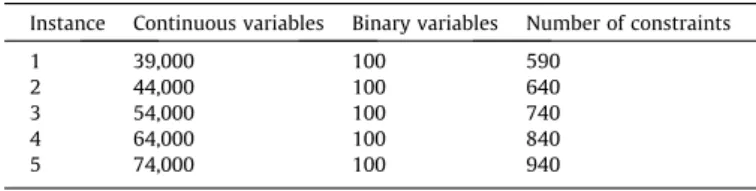
To illustrate the size differences between the problem instances of the RSCP model, for problem instances 1–5,Table 2shows the number of continuous and binary variables as well as the number of constraints.

5.2. Results analysis

InTable 3, the lower and upper bounds, gap (%), and number of Benders cycles are presented for Benders algorithmswithout any additional VI andwithVI of typewcon. These VI do not produce any significant impact, neither on the gap nor in the number of Benders cycles. To illustrate, for problem instance 3, gaps and

Fig. 3.Pseudo-code for a classical Benders decomposition algorithm with Pareto-optimal cuts.

(7)

Benders cycles are 0.869% and 9 respectively for both algorithms. When the algorithm hits the maximum number of Benders cycles (50), gaps provided by the Benders algorithms with cutswconis slightly lesser than those provided without any VI, except for prob-lem instance 9. This is a consequence of an upper bound slightly worse than that achieved by the Benders decomposition algorithm with VI of typewcon. To illustrate, for problem instance 4, the upper bounds are 3,357,200 and 3,354,300 for the Benders algo-rithmwithoutany VI andwithVI of typewcon, respectively. For

problem instance 5, gaps provided by both algorithms are the same. Regarding lower bounds, both algorithms present the same values.

InTable 4, the lower and upper bounds, gap (%) and number of Benders cycles are presented for Benders algorithm with VI of type

wcon1and for the alternative Benders algorithm with Pareto opti-mal cuts. The Benders algorithm with VI of typewcon1presents good results compared with the alternative Bender algorithm with Pareto optimal cuts. In some problem instances – for example, 2, 4, and 8 – gaps achieved by Benders algorithm with VI of typewcon1

are better than those provided by the alternative Benders algo-rithm. However, gaps are very similar between the two algorithms. Notice that for those instances, the alternative Benders algorithm has a smaller number of Benders cycles except for problem in-stance 4, where both algorithms have the same number. For prob-lem instances 1, 3, 5, 7, and 9–10, gaps provided by the alternative Benders algorithm are the best. In particular for problem instance 9, a network of 60010040, the alternative Benders algorithm required 13 Benders cycles to achieve a gap of 0.866%, while the Benders algorithm with VI of typewcon1required 50 Benders cy-cles – and hit the limit – to get a gap of 0.922%. However, inTable 8, we can observe that the smaller number of Benders cycles of the alternative Benders algorithm did not mean smaller computing times. On the contrary, the alternative Benders algorithm has the biggest computing times as a consequence of the time spending in solving the auxiliary problem to generate the Pareto optimal cuts. As observed by other authors, in our problem, the time spent to generate the optimal cuts at each iteration does not necessarily compensate with a reduction in the number of iterations and the total resolution time of the problem (Mercier & Soumis, 2007).

Table 5presents a summary of gaps and Benders cycles for the different Benders algorithms. To illustrate, for problem instance 9, gaps are 1.042%, 0.922%, 1.084% and 0.866% for the Benders algorithm without any VI, with VI of type wcon1,wconand the

Table 1 Data set.

# Instance problems |I| |K| |J| fk ai mk bj

1 35010040 350 100 40 2000 200 800 1750

2 40010040 400 100 40 2000 200 1500 2000

3 50010040 500 100 40 2000 200 1500 2500

4 60010040 600 100 40 2500 300 3000 2500

5 70010040 700 100 40 3000 300 3000 2500

6 35010040 350 100 40 20,000 200 800 1750

7 40010040 400 100 40 20,000 200 1500 2000

8 50010040 500 100 40 20,000 200 1500 2500

9 60010040 600 100 40 25,000 300 3000 2500

10 70010040 700 100 40 30,000 300 3000 2500

Table 2

Size formulation for problem instances 1–5.

Instance Continuous variables Binary variables Number of constraints

1 39,000 100 590

2 44,000 100 640

3 54,000 100 740

4 64,000 100 840

5 74,000 100 940

Table 3

Lower bound (zlb), upper bound (zub), gap and number of Benders cycles.

Instances Benders algorithm without any VI Benders algorithm with VIwcon

zlb zub Gap (%) Benders cycles zlb zub Gap (%) Benders cycles

1 2457900 2466000 0.330 5 2457900 2466000 0.330 5

2 2715200 2737200 0.810 22 2715200 2737200 0.810 22

3 3371300 3400600 0.869 9 3371300 3400600 0.869 9

4 3312700 3357200 1.343 50 3312700 3354300 1.256 50

5 3314000 3344500 0.920 50 3314000 3344500 0.920 50

6 4041900 4048550 0.165 6 4041900 4048550 0.165 4

7 3687200 3720100 0.892 9 3687200 3720100 0.892 7

8 4577300 4609900 0.712 7 4577300 4609900 0.712 5

9 4077700 4120200 1.042 50 4077600 4121800 1.084 50

10 4232000 4269000 0.874 9 4232000 4269000 0.874 8

Table 4

Lower bound (zlb), upper bound (zub), gap and number of Benders cycles.

Instances Benders algorithm – VIwcon1 Benders algorithm with Pareto optimal cuts

zlb zub Gap (%) Benders cycles zlb zub Gap (%) Benders cycles

1 2457900 2465050 0.291 2 2457900 2464300 0.260 2

2 2715200 2738000 0.840 24 2715200 2738600 0.862 22

3 3371300 3397800 0.786 10 3371300 3395700 0.724 12

4 3312700 3355400 1.289 50 3312700 3369000 1.700 50

5 3314000 3346500 0.981 21 3314000 3342000 0.845 22

6 4041900 4048500 0.163 2 4041900 4048500 0.163 2

7 3687200 3716600 0.797 4 3687200 3715400 0.765 4

8 4577300 4598700 0.468 5 4577300 4618300 0.896 4

9 4077700 4115300 0.922 50 4077700 4113000 0.866 13

10 4232000 4267000 0.827 7 4232000 4258500 0.626 5

(8)

alternative Benders algorithm with Pareto optimal cuts, respec-tively. For the same instance, the number of Benders cycles is 13 for the alternative Benders algorithm and 50 for all other algo-rithms. For problem instances 2, 4 and 8, the alternative Benders algorithm gap is worse than that obtained for the others’ algo-rithms. In all other cases, alternative Benders algorithms perform better in term of gaps and Benders cycles, except for the problem instances mentioned above. The minimum average number of Benders cycles is obtained by the alternative Benders decomposi-tion algorithm with Pareto optimal cuts, while the minimum aver-age gap is obtained by the Benders algorithm with VI of type

wcon1.

Table 6presents the initial (iLB) and the last lower bounds (zlb)

obtained by each Benders algorithm. Notice that the Benders algo-rithm with VI of typewcon1and the alternative Benders algorithm obtain the best lower bound in the first iteration (Benders cycle) of the algorithm. Comparing the other two Benders algorithms, we observe that there is not a significant difference between the lower bounds provided by them.Table 7shows the relative difference in percentage between the initial lower bound (iLB) and the last low-er bound (100[iLBzlb]/iLB) provided by the Benders algorithm

(withoutany VI) and the Benders algorithmwithVI of typewcon. This percentage represents an improvement percentage of the low-er bound ovlow-er the initial lowlow-er bound. Note that the maximum rel-ative difference is 71.5% and 70.3% for the Benders algorithm and the Benders algorithm with VI of typewcon,respectively.

Table 8reports the computational times (in seconds) required for the different Benders algorithms to obtain an integer solution within 0.9% of optimality. We observe that, in general, computa-tional times are mostly well below 91 s. The Benders decomposi-tion algorithm based on Pareto-optimal cuts presents the highest computational time. This is true for problem instances 2, 3, 4, 5,

8 and 10. We note that the Benders decomposition algorithm using

wcon1cuts in general performs well in terms of computational

Table 5

Summary gap and number of Benders cycles – different Benders decomposition algorithms.

Instances Without any VI VIwcon1 VIwcon Pareto-optimal cuts

Gap (%) Benders cycles Gap (%) Benders cycles Gap (%) Benders cycles Gap (%) Benders cycles

1 0.330 5 0.291 2 0.330 5 0.260 2

2 0.810 22 0.840 24 0.810 22 0.862 22

3 0.869 9 0.786 10 0.869 9 0.724 12

4 1.343 50 1.289 50 1.256 50 1.700 50

5 0.920 50 0.981 21 0.920 50 0.845 22

6 0.165 6 0.163 2 0.165 4 0.163 2

7 0.892 9 0.797 4 0.892 7 0.765 4

8 0.712 7 0.468 5 0.712 5 0.896 4

9 1.042 50 0.922 50 1.084 50 0.866 13

10 0.874 9 0.827 7 0.874 8 0.626 5

Ave 0.796 21.7 0.736 17.5 0.791 21 0.771 14.9

Max 1.343 50 1.289 50 1.256 50 1.700 50

Min 0.165 5 0.163 2 0.165 4 0.163 2

Table 6

Summary of initial and last lower bound – different Benders decomposition algorithms.

# Without any VI VIwcon1 VIwcon Pareto-optimal cuts

Initial Last Initial Last Initial Last Initial Last

1 2355500 2457900 2457900 2457900 2355500 2457900 2457900 2457900

2 2630200 2715200 2715200 2715200 2630200 2715200 2715200 2715200

3 3269800 3371300 3371300 3371300 3269800 3371300 3371300 3371300

4 3227000 3312700 3312700 3312700 3230200 3312700 3312700 3312700

5 3215000 3314000 3314000 3314000 3215000 3314000 3314000 3314000

6 2356300 4041900 4041900 4041900 2373900 4041900 4041900 4041900

7 2631200 3687200 3687200 3687200 2648200 3687200 3687200 3687200

8 3271800 4577300 4577300 4577300 3288800 4577300 4577300 4577300

9 3227700 4077700 4077700 4077700 3252600 4077600 4077700 4077700

10 3215000 4232000 4232000 4232000 3242000 4232000 4232000 4232000

Table 7

Relative difference between the initial and the last lower bound provided by Benders algorithms.

Instances Without any VI

relative difference (%)

VIwconrelative difference (%)

1 4.35 4.35

2 3.23 3.23

3 3.10 3.10

4 2.63 2.55

5 3.08 3.08

6 71.54 70.26

7 40.13 39.23

8 39.90 39.18

9 26.33 25.36

10 31.63 30.54

Table 8

Computational times (s) for the Benders algorithms.

Instances Without any VI

time (s)

VIwcon1 time (s)

VIwcon time (s)

Pareto-optimal cuts time (s)

1 4.219 1.708 4.156 3.056

2 13.853 14.543 14.096 30.458

3 7.715 8.580 7.739 21.422

4 35.480 30.628 31.646 91.731

5 34.643 34.361 34.552 44.324

6 4.797 1.896 3.244 3.167

7 6.739 3.144 5.110 5.802

8 6.901 4.390 4.851 7.462

9 34.345 30.869 32.033 31.070

(9)

times. This algorithm presents the smallest computational time for problem instances 1, 4, 5, 6, 7, 8, 9 and 10. For problem instances 2 and 3, the Benders decomposition algorithm usingwcon1cuts pre-sents the worst computational time. For our problem, considering the quality of the lower and upper bounds obtained by the Benders decomposition algorithm usingwcon1cuts and the computational time it spent in obtaining these bounds, the relative performance of this algorithm is good. Furthermore, as it was observed for other problems (Saharidis, Boile, & Theofanis, 2011; Tang et al., 2012), a strong valid inequality, like thewcon1, can help to accelerate the convergence of the Benders algorithm by providing an improved lower bound (the best lower bound in seven out of ten, excluding Benders algorithm with Pareto-optimal cuts) and that can also eventually compensate the increase in the total resolution time produced by the poor quality of the optimality cuts generated by the Benders subproblem (without using Pareto-optimal cuts).

6. Conclusions

In this paper, we analyzed a reverse and sustainable supply chain network design problem. This is a NP-hard combinatorial problem and it addresses the design of a supply network that con-sists of three types of members: sourcing facilities (sources), repro-cessing facilities, and reclamation facilities. We need to locate reprocessing facilities in order to minimize the flow cost from the origination sites to the reclamation facilities through repro-cessing facilities. We proposed Benders decomposition algorithms for solving the problem. In order to accelerate the convergence of the algorithm and to improve the quality of the lower bounds, we proposed two sets of valid inequalities. One of them proved to have a significant impact on the quality of the lower bound. As a second strategy to accelerate convergence of the algorithm, we derived quasi Pareto-optimal cuts and proposed a primal based Benders decomposition algorithm for solving the problem. Both algorithms were compared and, in some problem instances, in terms of the quality of lower and upper bounds, computational re-sults provided better performance for the primal based Benders decomposition algorithm with Pareto-optimal cuts. But in terms of total resolution time, this algorithm presents the highest values. As observed by other authors (for example,Mercier and Soumis, 2007; Sherali and Lunday, 2011), the time required to generate Pareto-optimal cuts does not necessarily offset the total resolution time. On the other hand, introducing awcon1valid inequality into the Master problem from the first iteration proved to be an effec-tive way to accelerate convergence; in addition, the first lower bound obtained by solving the Relaxed Master Problem was signif-icantly improved. This algorithm presents the smallest computa-tional time in eight out of ten problem instances. The final gap provided by this algorithm does not present a significance differ-ence (less than 0.2%) when compared with the best gap provided by the Benders algorithm with Pareto-optimal cuts. We can con-clude that, for this problem, a Benders algorithm with a strong va-lid inequality presents a good performance in terms of gap and total resolution time.

References

Altiparmak, F., Gen, M., Lin, L., & Paksoy, T. (2006). A genetic algorithm approach for multi-objective optimization of supply chain networks.Computers & Industrial Engineering, 51(1), 196–215.http://dx.doi.org/10.1016/j.cie.2006.07.011. Alumur, S. A., Nickel, S., Saldanha-da-Gama, F., & Verter, V. (2012). Multi-period

reverse logistics network design.European Journal of Operational Research, 220(1), 67–78.http://dx.doi.org/10.1016/j.ejor.2011.12.045.

Barbosa-Povoa, A. P., Salema, M. I. G., & Novais, A. Q. (2007). Design and planning of closed loop supply chains. In L. G. Papageorgiou & M. C. Georgiadis (Eds.),Supply chain optimization(pp. 187–218). Wiley.

Barros, A. I., Dekker, R., & Scholten, V. (1998). A two-level network for recycling sand: A case study.European Journal of Operational Research, 110(2), 199–214. http://dx.doi.org/10.1016/S0377-2217(98)00093-9.

Benders, J. F. (1962). Partitioning procedures for solving mixed-variables programming problems.Numerische Mathematik, 4(1), 238–252.

Bloemhof-Ruwaard, J., Salomon, M., & Van Wassenhove, L. N. (1996). The capacitated distribution and waste disposal problem. European Journal of Operational Research, 88, 490–503. <http://www.sciencedirect.com/science/ article/pii/0377221794002118>.

Cordeau, J.-F., Pasin, F., & Solomon, M. M. (2006). An integrated model for logistics network design.Annals of Operations Research, 144(1), 59–82.http://dx.doi.org/ 10.1007/s10479-006-0001-3.

Côté, G., & Laughton, M. A. (1984). Large-scale mixed integer programming: Benders-type heuristics. European Journal of Operational Research, 16(3), 327–333.http://dx.doi.org/10.1016/0377-2217(84)90287-X.

Daskin, M. S., Snyder, L. V., & Berger, R. T. (2005). Facility location in supply chain design. In A. Langevin & D. Riopel (Eds.), Logistics systems: Design and optimization(pp. 39–65). Kluwer.

Dogan, K., & Goetschalckx, M. (1999). A primal decomposition method for the integrated design of multi-period production–distribution systems. IIE Transactions, 31(11), 1027–1036.http://dx.doi.org/10.1080/07408179908969904. Farahani, R. Z., & Hekmatfar, M. (2009). Facility location: Concepts, models, algorithms

and case studies. In R. Zanjirani Farahani & M. Hekmatfar (Eds.),Media(pp. 549). Springer-Verlag. <http://www.dx.doi.org/10.1007/978-3-7908-2151-2>. Fleischmann, Moritz, Beullens, P., Bloemhof-Ruwaard, J. M., & Va, L. N. (2001). The

impact of product recovery on logistics network design. Production and Operations Management, 10(2), 156–173.

Fleischmann, Moritz (2003). Reverse logistics network structures and design. In V. D. R. Guide & L. N. Van Wassenhove (Eds.),Business aspects of closed-loop supply chains(pp. 117–135). New York: Carnegie Mellon University Press.

Fleischmann, Mortiz, Krikke, H. R., Dekker, R., & Flapper, S. D. P. (2000). A characterisation of logistics networks for product recovery. Omega, 28(6), 653–666.http://dx.doi.org/10.1016/S0305-0483(00)00022-0.

Geoffrion, A., & Graves, G. (1974). Multicommodity distribution system design by Benders decomposition.Management science, 20(5), 822–844.

Gomes, M. I., Barbosa-Povoa, A. P., & Novais, A. Q. (2011). Modelling a recovery network for WEEE: A case study in Portugal.Waste Management (New York, NY), 31(7), 1645–1660.http://dx.doi.org/10.1016/j.wasman.2011.02.023.

Guide, V. D. R., & Van Wassenhove, L. N. (2009). OR FORUM – The evolution of closed-loop supply chain research.Operations Research, 57(1), 10–18.http:// dx.doi.org/10.1287/opre.1080.0628.

Jayaraman, V., Guide, V. D. R., & Srivastava, R. (1999). A closed-loop logistics model for remanufacturing.Journal of the Operational Research Society, 50(5), 497–508. http://dx.doi.org/10.1057/palgrave.jors.2600716.

Jayaraman, Vaidyanathan, Patterson, R. A., & Rolland, E. (2003). The design of reverse distribution networks: Models and solution procedures. European Journal of Operational Research, 150(1), 128–149. http://dx.doi.org/10.1016/ S0377-2217(02)00497-6.

Krikke, H. R., Van Harten, A., & Schuur, P. C. (1999). Business case Océ: Reverse logistic network re-design for copiers.OR Spectrum, 21(3), 381–409.http:// dx.doi.org/10.1007/s002910050095.

Le Blanc, H. M., Fleuren, H. A., & Krikke, H. R. (2004). Redesign of a recycling system for LPG-tanks.OR Spectrum, 26(2), 283–304. http://dx.doi.org/10.1007/s00291-003-0145-3.

Li, N. (2011). Research on location of remanufacturing factory based on particle swarm optimization.MSIE 2011(pp. 1016–1019). IEEE. doi:http://dx.doi.org/ 10.1109/MSIE.2011.5707588.

Listesß, O., & Dekker, R. (2005). A stochastic approach to a case study for product recovery network design. European Journal of Operational Research, 160(1), 268–287.http://dx.doi.org/10.1016/j.ejor.2001.12.001.

Lu, Z., & Bostel, N. (2007). A facility location model for logistics systems including reverse flows: The case of remanufacturing activities.Computers & Operations Research, 34(2), 299–323.http://dx.doi.org/10.1016/j.cor.2005.03.002. Magnanti, T., & Wong, R. (1981). Accelerating Benders decomposition: Algorithmic

enhancement and model selection criteria.Operations Research, 29(3), 464–484. <http://www.or.journal.informs.org/content/29/3/464.short>.

McDaniel, D., & Devine, M. (1977). A modified Benders partitioning algorithm for mixed integer programming.Management Science, 24, 312–319.

Mercier, A., & Soumis, F. (2007). An integrated aircraft routing, crew scheduling and flight retiming model.Computers & Operations Research, 34(8), 2251–2265. http://dx.doi.org/10.1016/j.cor.2005.09.001.

Neto, Q. F., Walther, G., Bloemhof-Ruwaard, J. M., Van Nunen, J. A. E. E., & Spengler, T. (2010). From closed-loop to sustainable supply chains: The WEEE case. International Journal of Production Research, 15, 4463–4481.

Papadakos, N. (2008). Practical enhancements to the Magnanti-Wong method. Operations Research Letters, 36(4), 444–449.

Rei, W., Cordeau, J.-F., Gendreau, M., & Soriano, P. (2008). Accelerating Benders decomposition by local branching. INFORMS Journal on Computing, 21(2), 333–345.http://dx.doi.org/10.1287/ijoc.1080.0296.

Saharidis, G. K. D., Boile, M., & Theofanis, S. (2011). Initialization of the Benders master problem using valid inequalities applied to fixed-charge network problems. Expert Systems with Applications, 38(6), 6627–6636. http:// dx.doi.org/10.1016/j.eswa.2010.11.075.

Saharidis, G. K. D., Minoux, M., & Ierapetritou, M. G. (2010). Accelerating Benders method using covering cut bundle generation. International Transactions in Operational Research, 17(2), 221–237.

(10)

Sahyouni, K., Savaskan, R. C., & Daskin, M. S. (2007). A facility location model for bidirectional flows.Transportation Science, 41(4), 484–499.http://dx.doi.org/ 10.1287/trsc.1070.0215.

Salema, M. I. G., Barbosa-Povoa, A. P., & Novais, A. Q. (2010). Simultaneous design and planning of supply chains with reverse flows: A generic modelling framework.European Journal of Operational Research, 203(2), 336–349.http:// dx.doi.org/10.1016/j.ejor.2009.08.002.

Sherali, H. D., & Lunday, B. J. (2011). On generating maximal nondominated Benders cuts. Annals of Operations Research. http://dx.doi.org/10.1007/s10479-011-0883-6.

Shih, L.-H. (2001). Reverse logistics system planning for recycling electrical appliances and computers in Taiwan. Resources Conservation and Recycling, 32(1), 55–72.http://dx.doi.org/10.1016/S0921-3449(00)00098-7.

Simchi-Levi, D., Kaminsky, P., & Simchi-Levi, E. (2007).Designing and managing the supply chain(3rd ed., Vol. 3). New York: McGraw-Hill/Irwin (pp. 354). New York: McGraw-Hill/Irwin.

Sodhi, M. S., & Reimer, B. (2001). Models for recycling electronics end-of-life products.OR Spectrum, 23, 97–115.

Tang, L., Jiang, W., & Saharidis, G. K. D. (2012). An improved Benders decomposition algorithm for the logistics facility location problem with capacity expansions.Annals of Operations Research.http://dx.doi.org/10.1007/ s10479-011-1050-9.

Tragantalerngsak, S., Holt, J., & Rönnqvist, M. (2000). An exact method for the two-echelon, single-source, capacitated facility location problem.European Journal of Operational Research, 123, 473–489. <http://www.sciencedirect.com/science/ article/pii/S0377221799001058>.

Wentges, P. (1996). Accelerating Benders’ decomposition for the capacitated facility location problem.Mathematical Methods of Operations Research, 44(2), 267–290.