Efficient Clustering of Web-Derived Data Sets
Lu´ıs Sarmento
Fac. Engenharia Univ. Porto Rua Dr. Roberto Frias, s/n
4200-465 Porto Portugal
[email protected]
Alexander P. Kehlenbeck
Google Inc. NYC 79, 9th Ave., 10019 NYC
New York, NY USA
[email protected]
Eug ´enio Oliveira
Fac. Engenharia Univ. Porto Rua Dr. Roberto Frias, s/n
4200-465 Porto Portugal
[email protected]
Lyle Ungar
Computer and Inf. Science Univ. of Pennsylvania 504 Levine, 200 S. 33rdSt
Philadelphia, PA USA
[email protected]
ABSTRACT
Many data sets derived from the web are large, high-dimensional, sparse and have a Zipfian distribution of both classes and features. On such data sets, current scalable clustering methods such as streaming clustering suffer from fragmen-tation, where large classes are incorrectly divided into many smaller clusters, and computational efficiency drops signif-icantly. We present a new clustering algorithm based on connected components that addresses these issues and so works well on web-type data.
1. INTRODUCTION
Clustering techniques are used to address a wide variety of problems using data extracted from the Web. Document clustering has long been used to improve Web IR results [21] or to detect similar documents on the Web [5]. More recently web-navigation log data has been clustered to provide news recommendation to users [8]. Several clustering-based ap-proaches have been proposed for named-entity
disambigua-tion some of them specifically dealing with web extracted
from the Web [20], [18].
Clustering data sets derived from the web - either docu-ments or information extracted from them - provides several challenges. Web-derived data sets are usually very large, easily reaching several million of items to cluster and ter-abyte sizes. Also, there is often a significant amount of noise due to difficulties in document pre-processing such as html boiler-plate removal and feature extraction.
More fundamentally, web-derived data sets have specific data distributions, which are not usually found in other datasets, that impose special requirements on clustering ap-proaches. First, web-derived datasets usually involve sparse,
high-dimensional features spaces (e.g., words). In such spaces,
comparing items is particularly challenging, not only be-cause of problems arising from high-dimensionality [1], but also because most vectors in sparse spaces will have similar-ities close to zero. For example, some clustering-based ap-proaches to named-entity disambiguation use co-occurring
Copyright is held by the author/owner(s).
WWW2009, April 20-24, 2009, Madrid, Spain. .
names as features for describing mentions (i.e. the occur-rence of a name ni in a document dk) for disambiguation.
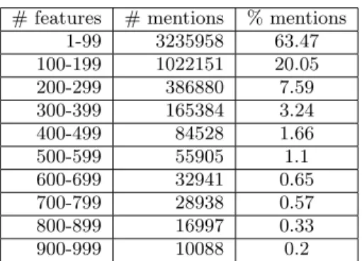
On a small Web sample of 2.6 million name-annotated doc-uments, we found 5.1 million mentions corresponding to 52,000 names. (I.e., the feature space is has dimension 52,000.) About 63% of the mentions we are trying to cluster have fewer than 100 features, and another 20% have between 100 and 199. As can be seen from Table 1, the vast major-ity of items have fewer than 1% of the possible features. On the open Web, the set of possible names - and hence the feature space dimensionality - is on the order of millions, so sparsity becomes specially problematic for clustering-based named-entity disambiguation approaches.
# features # mentions % mentions
1-99 3235958 63.47 100-199 1022151 20.05 200-299 386880 7.59 300-399 165384 3.24 400-499 84528 1.66 500-599 55905 1.1 600-699 32941 0.65 700-799 28938 0.57 800-899 16997 0.33 900-999 10088 0.2
Table 1: Distribution of the number features in men-tion vectors extracted from a 5.2 million documents web sample
The class distributions of the web-derived data are usually
highly unbalanced (often Zipfian), with one or two dominant
classes and a long tail of smaller classes. Let us consider again the problem of named-entity disambiguation. A name such as “Paris”, can refer to many possible entities. In fact, the Wikipedia disambiguation page for “Paris” (http:// en.wikipedia.org/wiki/Paris_(disambiguation)) shows more than 80 possible entities. (And doesn’t include hun-dreds of less well known people.) However, most of the men-tions of “Paris” found on the web refer either to the capital of France or to the famous socialite Paris Hilton. Table 2 shows hit counts for five queries sent to Google containing
Figure 1: The highly unbalanced distribution of the number features in mention vectors.
the word “Paris” and additional (potentially) disambiguat-ing keywords. These values are merely indicative of the or-ders of magnitude at stake, since hit counts are known to change significantly over time.
# query # hit count (x106) %
paris 583 100
paris france 457 78.4
paris hilton 58.2 9.99
paris greek troy 4.130 0.71
paris mo 1.430 0.25
paris tx 0.995 0.17
paris sempron 0.299 0.04
Table 2: Number of hits obtained for several entities named “Paris”
For other entities named “Paris” (for example, the French battleship), Google results are clearly contaminated by the dominant entity (the French capital) and thus it becomes almost impossible to estimate their relative number of hits. This also causes a problem for clustering algorithms, which need to be able to deal with such an unbalanced distribution in web-derived data, and still correctly cluster items of non-dominant classes.
Additionally, methods to cluster such large data sets have to deal with the fact that “all-against-all” comparison of items is impossible. In practice, items can only be com-pared to cluster summaries (e.g., centroids) or to only a few other items. The most widely used methods for clustering extremely large data sets are streaming clustering methods [10] that compare items against centroids. Streaming clus-tering has linear computational complexity and (under ideal conditions) modest RAM requirements. However, as we will show later, standard streaming clustering methods are less than ideal for web-derived data because of the difficulty in comparing items in high-dimensional, sparse and noisy spaces. As a result, they tend to produce sub-optimal solu-tions where classes are fragmented in many smaller clusters. Additionally, their computational performance is degraded by this excessive class fragmentation.
We propose a clustering algorithm that has performance comparable to that of streaming clustering for well-balanced data sets, but that is much more efficient for the sparse, un-evenly sized data sets derived from the web. Our method relies on an efficient strategy for comparing items in high
dimensional spaces that ensures that only the minimal suf-ficient number of comparisons is performed. A partial link-graph of connected components of items is built which takes advantage of the fact that each item in a large cluster only needs be compared with a relatively small number of other items. Our method is robust to variation in the distribution of items across classes; in particular, it efficiently handles Zipfian distributed data sets, reducing fragmentation of the dominant classes and producing clusters whose distributions are similar to the distribution of true classes.
2. STREAMING CLUSTERING OF WEB DATA
For the purpose of explaining the limitations of streaming clustering for web-derived data sets, we will consider a sin-gle pass of a simplified streaming clustering algorithm. This simplification only emphasizes the problems that stream-ing clusterstream-ing algorithms face, while not changstream-ing the basic philosophy of the algorithm. In Section 2.3 we will show that this analysis can be extended to realistic streaming-clustering approaches. The simplified version of the stream-ing clusterstream-ing algorithm we will be usstream-ing is as follows:
1. shuffle all items to be clustered and prepare them for sequential access;
2. while there are unclustered items, do: (a) take the next unclustered item;
(b) compare with all existing cluster centroids; (c) if the distance to the closest centroid is less that
mindist, add the item to the closest cluster and
update the corresponding centroid;
(d) otherwise, create a new cluster containing this item only.
The time and space complexity analysis of this algorithm is straight-forward. For n items to be clustered and if Cf
clusters are found, this algorithm will perform in O(n Cf)
time, since each item is only compared with the centroids of the Cf existing clusters, and in O(Cf) space: we only need
to store the description of the centroid for each clusters.
2.1 Problems arising from False Negatives
The high dimensionality and sparseness of web-derived the data hurts streaming clustering because when compar-ing two items with sparse features there is a non negligi-ble probability of those items not sharing any common at-tribute. This is so even when the items being compared belong to the same class.
Such false negatives have a very damaging effect on stream-ing clusterstream-ing. If a false negative is found while performstream-ing comparisons between an item to be clustered and existing cluster centroids, the streaming clustering algorithm will as-sume that the item belongs to an as yet unseen class. In such cases a new cluster will be created to accommodate it. This will lead to an artificial increase in the number of clusters that will be generated for each class, with two direct conse-quences:
1. during streaming, clustered items will have to be pared with additional clusters, which will degrade com-putational performance in time and space; and
2. the final clustering result will be composed of multiple clusters for each class, thus providing a fragmented solution
Whether this degradation is significant or not depends ba-sically on how probable it is to find a false negative when comparing items with existing clusters. Our claim is that on web generated data the probability is in fact quite large since the dimensionality of the spaces is very high and vec-tor representations are very sparse. To make matters worse, fragmentation starts right at the beginning of the clustering process because most items will have nothing in common with the early clusters.
2.2 The Impact of False Negatives
To make a more rigorous assessment of the impact of false negatives on the performance of streaming clustering, let us consider only the items belonging to one specific arbitrary class, class A. In the beginning no clusters exist for items of class A, so the first item of that class generates a new cluster, Cluster 1. The following elements of class A to be clustered will have a non-zero probability of being a false negatives. i.e, of not being correctly matched with the already existing cluster for class A. (We assume for now that there are no false positives, i.e. that they will not be incorrectly clustered with elements of other classes.) In this case a new cluster, Cluster 2, will be generated.
The same rationale applies when the following items of class A are compared with existing clusters for that class. We assume that in any comparison, there is a probability pf n
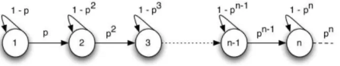
of incorrectly mismatching the item with a cluster. There-fore, one expects new clusters for class A to be generated as more items are processed by streaming clustering. This behavior can be modeled by an infinite Markov Chain as depicted in Figure 2.
Figure 2: Markov model for fragmentation in streaming clustering
The probability of having created l clusters after perform-ing streamperform-ing clusterperform-ing for n + 1 items is the probability of being in a given state s (1, 2, 3, ...) of the chain. Assuming independence, as more clusters are generated the probabil-ity of creating a new (false) cluster decreases exponentially because that would require more consecutive false negative comparisons.
Despite the regularities of this Markov Chain, deriving general expressions for the probability of a given state af-ter n iaf-terations is relatively hard except for trivial cases (see [19]). However, for the purpose of our analysis, we can perform some simplifications and obtain numeric values for comparison. By truncating the size of a chain to a maximum length (smax) and changing the last state of the chain to
become an “absorbing state” that represents all subsequent states, numeric computation of state probabilities becomes straight-forward for any value of p. Table 3 shows the most probable state, smp and its corresponding probability, pmp
after clustering 10,000 and 100,000 items (with smax= 16)
for various values of pf n:
pf n smp(10k) pmp(10k) smp(100k) pmp(100k) 0.2 6 0.626 8 0.562 0.3 8 0.588 10 0.580 0.4 10 0.510 13 0.469 0.5 13 0.454 16 0.844 0.6 16 0.941 16 1.000
Table 3: Most probable state of the Markov chain, for 10k and 100k items clustered and different prob-abilities of false negatives, pf n
As can be easily seen, even for very low probabilities for false negatives (pf n ≤ 0.3), the chances of replicating the
number of clusters several times is considerable. In a realis-tic scenario, values of pf n > 0.5 can easily occur for
domi-nant classes because item diversity in those clusters can be very significant. Therefore, when performing streaming clus-tering in such conditions, cluster fragmentation of at least one order of magnitude should be expected.
2.3 Impact on Realistic Streaming Clustering
Actual streaming clustering implementations attempt to solve the fragmentation problems in two ways. The first option is to perform a second pass for clustering the frag-mented clusters based on their centroids. The problem with this is that the information that could be used for safely connecting two clusters (i.e., the points in between them) has been lost to centroid descriptions, and these might be too far apart to allow a safe merge since centroids of other clusters may be closer. (See the illustration in Figure 3). This situation can more easily occur for large clusters in high-dimensional and sparse spaces, where sub-clusters of items might be described by almost disjoint sets of features, and thus be actually distant in the hyperspace. Thus, for
web derived data, re-clustering will not necessarily solve the
fragmentation problem, although such an approach is often successful in lower-dimensional and homogeneous datasets.
Figure 3: Centroids of belonging to fragments of the same clusters might be more distant than those belonging to different clusters.
A second variation of streaming clustering algorithms keeps a larger number of clusters than the final target, and alter-nates between adding more new items to clusters and con-sidering current clusters for merging. However, if each of the items included in the cluster has a sparse representa-tion, and if such “intermediate” clusters have a high level of intra-cluster similarity (as they are supposed to be in or-der to avoid adding noisy items), then the centroids will probably also have a sparse feature representation. As more items are clustered, each of these many intermediate clusters will tend have only projections in small set of features, i.e.
those of the relatively few and very similar items it contains. Therefore, feature overlap between clusters will tend to be low, approximately in the same way item feature overlap is low. Such centroids will thus suffer from the same false negative problems as individual items do, and the number of potential clusters to hold in memory may grow large. In practice, unless one reduces the minimum inter-cluster sim-ilarity for performing merge operations (which could lead to noisy clusters), this strategy will not lead to as many clus-ter merging operations as expected, and many fragmented clusters will persist in the final solution. Again, the frag-mentation effect should be more visible for larger clusters, in high-dimensional and sparse space.
3. CLUSTERING BY FINDING CONNECTED
COMPONENTS
In this section we present a scalable clustering method that is robust to the previously described problems. It is easy to understand that overcoming the problems generated by false negatives involves changing the way comparisons are made; Somehow we need to obtain more information about similarity between items to compensate the effect of false negatives, but that needs to be done without compromising time and space restrictions.
Complete information about item similarity is given by the Link Graph, G, of the items. Two items are linked in
G if their level of pair-wise similarity is larger than a given
threshold. The information contained in the Link Graph should allow us to identify the clusters corresponding to the classes. Ideally, items belonging to the same class should exhibit very high levels of similarity and should thus be-long to the same connected component of G. On the other hand, items from different classes should almost never have any edges connecting them, implying the they would not be part of the same connected components. In other words, each connected component should be a cluster of items of the same class, and there should be a 1-1 mapping between connected components (i.e. clusters) and classes.
Clustering by finding connected-components is robust to the problem of false negatives, because each node in G is ex-pected to be linked to several other nodes (i.e. for each item we expect to find similarities with several other nodes). The effect of false negatives could be modeled by randomly re-moving edges from G. For a reasonably connected G, random edge removal should not affect significantly the connectivity within the same connected component, since it is highly un-likely that all critical edges get removed simultaneously. The larger the component, the more unlikely it is that random edge removal will fragment that component because more connectivity options should exist. Thus, for web-derived data sets, where the probability of false negatives is non-negligible, clustering by finding the connected-components of the link graph seems to be an especially appropriate op-tion.
Naive approaches to building G would attempt an all-against-all comparison strategy. For large data sets that would certainly be infeasible due to time and RAM limita-tion. However, an all-against-all strategy is not required. If our goal is simply to build the Link Graph for finding the true connected components then we only need to ensure that we make enough comparisons between items to obtain a
suf-ficiently connected graph, Gmin, which has the same set of
connected components as the complete Link Graph G. This means that Gminonly needs to contain the sufficient number
of edges to allow retrieving the same connected components as if a complete all-against-all comparison strategy had been followed. In the most favorable case, Gmincan contain only
a single edge per node and still allow retrieving the same connected components as in G (built using an all-against-all comparisons strategy).
Since efficient and scalable algorithms exist for finding the connected components of a graph ([7], [12]), the only addi-tional requirement needed for obtaining a scalable clustering algorithm that is robust to the problem of false negatives is a scalable and efficient algorithm for building the link graph. We propose one such solution in the next section.
3.1 Efficiently Building the Link Graph
GOur goal at this step is to obtain a sufficiently connected Link Graph so we can then obtain clusters that correspond to the original classes without excessive fragmentation. We will start by making the following observation regarding web derived data sets: because the distribution of items among class is usually highly skewed, then for any item that we randomly pick belonging to a dominant class (possibly only one or two) we should be able to rather quickly pick another item that is “similar” enough to allow the creation of an edge in the link graph. This is so even with the finite probability of finding false negatives, although such negatives will force us to test a few more elements. In any case, for items in the dominant classes one can establish connections to other items with vastly fewer comparisons than used in an all-against-all comparison scheme. We only need enough con-nections (e.g., one) to ensure enough connectivity in order to later retrieve the original complete connected components.
For the less frequent items many more comparisons will be needed to find another “similar enough” item, since such items are, by definition, rare. But since rare items are rare, the total number of comparisons is still much lower than what is required under a complete all-against-all-strategy.
We use a simple procedure: for each item keep comparing it with the other items until kpossimilar items are found, so
as to ensure enough connectivity in the Link Graph. More formally:
1. Shuffle items in set S(n) to obtain Srand(n).
2. Give sequential number i to each item in Srand(n)
3. Repeat for all the items starting with i = 0: (a) take item at position i, ii
(b) Set j = 1
(c) Repeat until we find kpos positive comparisons
(edges)
i. Compare item iiwith item ii+j
ii. Increment j
One can show (Appendix A) that the average computation cost under this “amortized comparison strategy” is:
˜ O „ n · |C| · kpos 1 − pf n « (1) with n the number of items in the set, |C| the number of different true classes, pf nis the probability of false negatives
and kposas the number of positive comparisons,
correspond-ing to the number of edges we wish to obtain for each item. This cost is vastly lower than what would be required for a blind all-against-all comparison strategy, without signifi-cantly reducing the chances of retrieving the same connected components. Notice that computation cost is rather stable to variation of pf n when pf n < 0.5. For pf n = 0.5 the
cost is just the double of the ideal case (pf n= 0), which is
comparatively better than values presented in Table 3. One can also show that the expected value for the maxi-mum number of items that have to be kept in memory during the comparison strategy, nRAM is equal to:
E(nRAM) = kpos
pmin· (1 − pf n) (2)
where pminis the percentage of items of the smallest class.
This value depend solely on the item distribution for the smallest class and on the probability of false negatives, pf n.
If only 0.1% of the elements to be clustered belong to the the smallest class kpos= 1, and pf n= 0.5 then E(nRAM) =
2000. It is perfectly possible to hold information in RAM that many vectors with standard computers. Imposing a hard-limit on this value (for e.g. 500 instead of 2000) will mostly affect the connectivity for less represented classes.
Another important property of this strategy is that link graphs produced this way do not depend too much on the order by which items are picked up to be compared. One can easily see that, ideally (i.e., given no false negatives), no matter which item is picked up first, if we were able to correctly identify any pair of items of the same class as sim-ilar items, then the link graph produced would contain ap-proximately the same connected components although with different links. In practice, this will not always be the case because false negatives may break certain critical edges of the graph, and thus make the comparison procedure order-dependent. A possible solution for this issue is to increase the number of target positive comparison to create more alternatives to false negative and thus reduce the order de-pendency.
3.2 Finding Connected Components
Given an undirected graph G with vertices {Vi}i=1..N and
edges {Ei}i=1..K, we wish to identify all its connected
com-ponents; that is, we wish to partition G into disjoint sets of vertices Cj such that there is a path between any two
vertices in each Cj, and such that there is no path between
any two vertices from different components Cj and Ck.
There is a well-known [7] data structure called a disjoint-set forest which naturally solves this problem by maintaining an array A of length N of representatives, which is used to identify the connected component to which each vertex belongs. To find the representative of a vertex Vi, we apply
the function Find(x) {
if(A[x] == x) return x; else return Find(A[x]); }
starting at i. Initially A[i] = i for all i, reflecting the fact that each vertex belongs to its own component. When an edge connecting Viand Vjis processed, we update A[F ind(i)] ←
F ind(j).
This naive implementation offers poor performance, but it can be improved by applying both a rank heuristic, which
determines whether to update via A[F ind(i)] ← F ind(j) or
A[F ind(j)] ← F ind(i) when processing a new edge and path compression, under which F ind(i) sets each A[x] it ever
vis-its to be the final representative of x. With these improve-ments, the runtime complexity of a single Find() or update operation can be reduced to O(α(N )), where α is the inverse of the (extremely fast-growing) Ackermann function A(n, n) [7]. Since A(4, 4) has on the order of 2(1019729)digits, α(N ) is effectively a small constant for all conceivably reasonable values of N .
4. EXPERIMENTAL SETUP
We compared the (simplified) streaming clustering (SC) algorithm with our connected component clustering (CCC) approach on artificially generated data-sets. Data-sets were generated with properties comparable to web-derived data, namely:
• Zipfian distribution of class sizes, with one or two
dom-inant classes;
• The number of features associated with each class
in-creases sub-linearly with class size.
• The number of non-negative features in each item is
Zipfian distributed, and larger for larger classes. (Items have at least three non-negative features).
• The feature distribution inside each class is lightly Zip-fian (exponent 0.5), meaning that there is a subset of
features that occurs more frequently but often enough to make them absolutely discriminant of the class. Each class has its own set of exclusive features. Therefore, in the absence of noise, items of different classes will never share any feature and thus will always have 0 similarity. Overlap between items of different classes can be achieved by adding noisy features, shared by all classes. A given proportion of noise features can be randomly added to each item.
To ensure a realistic scenario, we generated a test set with 10,000 items with Zipfian-like item distribution over 10 classes. Noise features were added so that clustering would have to deal with medium level noise. Each item had an ad-ditional 30% noise features added, taken from a noise class with 690 dimensions. Noise features have a moderately de-caying Zipfian distribution (exponent 1.0). Table 4 shows some statistics regarding this test set, S30. We show the average number of features per item, avg(#ft), and the av-erage number of noise features per item, avg(#ftnoise). Pno
is the probability of not having any overlap if we randomly pick two items from a given class (this should be a lower bound for Pf n).
4.1 Measures of Clustering Performance
The evaluation of the results of clustering algorithms is a complex problem. When no gold standard clusters are avail-able the quality of clustering can only be assessed based on internal criteria, such as intra-cluster similarity which should be as high, and inter-cluster similarity, which should be as low. However, these criteria do not necessarily im-ply that the clusters obtained are appropriate for a given practical application [15].
Class Items dim avg(#ft) avg(#ftnoise) Pno 1 6432 657 54.14 15.95 0.53 2 1662 556 48.25 14.14 0.56 3 721 493 44.13 12.88 0.56 4 397 448 39.83 11.60 0.58 5 249 413 34.04 9.84 0.57 6 187 392 34.70 10.06 0.59 7 133 366 35.03 10.18 0.58 8 87 334 29.64 8.56 0.58 9 77 325 26.71 7.61 0.61 10 55 300 24.6 7.05 0.61
Table 4: Properties of the test set S30 When gold standard clusters are available one can perform evaluation based on external criteria by comparing cluster-ing results with the existcluster-ing gold standard. Several metrics have been proposed for measuring how “close” test clusters are to reference (gold standard) clusters. Simpler metrics are based frequency counts regarding how individual items [22] or pairs of items [11, 17] are distributed among test clusters and gold standard clusters. These measures, how-ever, are not invariant under scaling, i.e., they are sensitive to the number of items being evaluated so we opted for two information-theoretic metrics, which depend solely on item distribution.
Given a set of |T | test clusters T to be evaluated, and a gold standard, C, containing the true mapping from the items to the |C| classes, we wish to evaluate how well clusters in T , t1, t2,...t|T | represent the classes in C, c1, c2,... c|c|.
Ideally, all the items from any given test cluster, tx, should
belong to only one class. Such a tx cluster would then be
considered “pure” because it only contains items of a unique class as defined by the Gold Standard. On the other hand, if items from txare found to belong to several gold standard
classes, then the clustering algorithm was unable to correctly separate classes. To quantify how elements in test cluster tx
are spread over the true classes, we will measure the entropy of the distribution of the elements in tx over all the true
classes, cy. High quality “pure” clusters should have very
low entropy values.
Let ixy be the number of items from test cluster tx that
belong to class cyand let |tx| be the total number of elements
of cluster tx(that can belong to any of the |C| true classes).
The cluster entropy of the test cluster tx over all |C| true
classes is: et(tx) = |C| X y=0 −ixy |tx| · ln(ixy |tx| ) (3)
For all test clusters under evaluation we can compute Et,
the weighted average of the entropy of each individual test cluster, e(tx): Et= P|T | x=0|tx| · et(tx) P|T | x=0|tx| (4) In the most extreme case, all test clusters would have a single element and be “pure”. This, however, would mean that no clustering had been done, so we need to simultane-ously measure how elements from the true classes are spread throughout the test clusters. Again, we would like to have all items from a given true class in the fewest test clusters possible, ideally only one. Let |cy| the the number of items
in class cy. Then, for each true class, cy, we can compute the
class entropy, i.e. the entropy of the distribution of items of
such class over the all test clusters by:
ec(cy) = |T | X x=0 −ixy |cy| · ln(ixy |cy| ) (5)
A global clustering performance figure can be computed as a weighted average over all classes of each individual class
entropy Ec= P|C| y=0|cy| · ec(cy) P|C| y=0|cy| (6) We would like to simultaneously have Et and Ecas close
to zero as possible, meaning that test clusters are “pure” and that they completely represent the true classes. In the case of a perfect clustering (a 1-to-1 mapping between clusters and classes), both Et and Ecwill be 0.
5. RESULTS
We compared the performance of our connected compo-nents clustering (CCC) algorithm with two other algorithms: simplified 1-pass stream clustering (1p-SC) and 2-pass stream-ing clusterstream-ing (2p-SC). The simplified 1-pass streamstream-ing clus-tering was described in Section 3 and was included in the comparison for reference purposes only. The 2-pass stream-ing clusterstream-ing consists in performstream-ing a re-clusterstream-ing of the clusters obtained in the 1-pass, using information about the centroids of the clusters obtained. The re-clustering is made using the exact same stream-clustering procedure, merging clusters using their centroid information. The 2-pass SC algorithm is thus a closer implementation of the standard streaming clustering algorithm.
Each of the algorithms has parameters to be set. For the CCC algorithm we have three parameters that control how the “amortized comparison strategy” is made: (i) minimum
item similarity, smincc; (ii) target positive comparisons for
each item, kpos; and (iii) maximum sequence of comparisons
that can be performed for any item, kmax (which is
equiv-alent to the maximum number of items we keep simulta-neously in RAM). The kposand kmax parameters was kept
constant in all experiments: kpos = 1, kmax = 2000 (see
Section 3.1).
The 1-pass SC algorithm has only one parameter, sminp1, which is the minimum distance between an item and a clus-ter centroid to merge it to that clusclus-ter. The 2-pass SC algo-rithm has one additional parameter in relation to the 1-pass SC. sminp2controls the minimum distance between the cen-troids for the corresponding clusters to be merged together in the second pass. The vector similarity metric used in all algorithms was the Dice metric.
Since all algorithms depend on the order of the items be-ing processed, items were shuffled before bebe-ing clustered. This process (shuffling and clustering) was repeated 5 times for each configuration. All Results shown next report the average over 5 experiments.
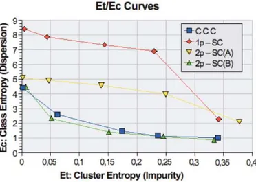
Figure 4 shows the Et (“cluster impurity”), Ec (“class
dispersion”) curves obtained for the three algorithms, using the test set S30. Results were obtained by changing smincc,
sminp1 and sminp2, from relatively high values that ensured almost pure yet fragmented clusters (Et≈ 0 but Ec>> 0)
noisier clusters (Ec< 1 but Et>> 0). We compared the
re-sults of the CCC algorithm with rere-sults obtained from the 1-pass SC (1p-SC) and two different configuration for the two pass stream-clustering algorithm: 2p-SC(A) and 2p-SC(B). Configuration 2p-SC(A) was obtained by changing sminp2 while keeping the value sminp1 constant at a level that en-sured that the partial results from the first pass would have high purity (yet very high fragmentation). For the configu-ration 2p-SC(B), we followed for a different strategy for set-ting parameters: we kept sminp2constant at a medium level, and slowly decreased sminp1 to reduce the fragmentation of partial clusters. Configuration 2p-SC(B) was found to the best performing combination among all (several dozens) of configuration tried for the two pass clustering algorithm.
Since we manually verified that, for this test set, values of Et larger than 0.3 indicate that the clusters produced
are mixing items from different classes, Figure 4 only shows results for Et< 0.4.
Figure 4: Ec(y-axis) vs. Et(x-axis) for four
cluster-ing methods (see text). CCC gives much better re-sults than most streaming clustering configurations, and is comparable to a carefully tuned streaming method.
We made further comparisons between our CCC algo-rithm and the best performing configuration of the 2p-SC al-gorithm. Table 5 shows the results of this comparison when aiming at a target value of Et= 0.15. Relevant criteria for
comparing clustering quality are the Et and Ec values, the
number of clusters generated (# clusters) and the number of singleton clusters (# singleton) produced. For compar-ing computational performance we present the number of comparisons made (# comparisons) and the overall execu-tion time of each algorithm. For 2p-SC we show statistics regarding both the intermediate results (i.e., after pass 1) and the final results (after pass 2), so as to emphasize their relative contributions.
Table 6 shows a typical example of the cluster / true class distribution of the top 10 clusters for the results obtained. (Compare with Table 4). The existence of two or more clus-ters for Class 1 (and sometimes also for Class 2) was a com-mon result for the 2p-SC algorithm.
2p-SC (pass 1) 2p-SC (final) CCC Et 0.08 0.15 0.15 Ec 7.64 1.1 1.53 # clusters 755.4 184 647.6 # singletons 66.4 66.4 478.2 # comparisons 4.2M 74k 2.2M t (secs.) 142 4 42
Table 5: Comparison between 2p-SC and CCC for target cluster purity Et= 0.15.
CCC 2p-SC
Cluster True Class [#Items] True Class [#Items]
1 1 [6113] 1 [3302] 2 2 [1405] 1 [3087] 3 3 [582] 2 [1573] 4 4 [321] 3 [636] 5 5 [170] 4 [323] 6 6 [134] 5 [192] 7 7 [96] 6 [150] 8 9 [40] 7 [100] 9 4 [38] 8 [68] 10 8 [37] 9 [58] 11 1 [32] 10 [36] 12 10 [30] 2 [18]
Table 6: Typical cluster / true class distribution for target cluster purity Et= 0.15. Note that streaming
clustering (2p-SC) splits class 1 across two clusters.
6. ANALYSIS OF RESULTS
The results plotted in Figure 4 show that the connected components clustering (CCC) algorithm we propose gives clustering qualities very close to those of the best perform-ing 2p-streamperform-ing clusterperform-ing approach (2p-SC). Additionally, the CCC algorithm consistently required approximately only
half the number of comparisons to produce results
compa-rable to the 2p-SC, as the first pass of streaming clustering tends to generate heavy fragmentation (and hence Ec> 6).
This is especially the case for the relevant part of the Et /
Ec curve (Et ≤ 0.3); Thus, we can obtain a significant
im-provement in computational performance in the regime we most care about.
The results in Table 5 suggest that in practice, CCC may have better results than 2p-SC. The Ec(fragmentation)
val-ues that the CCC algorithm obtains are worsened by the extremely large tail of singleton or very small clusters that are produced. (These are outliers and items in the end of the buffer that ended up not having the chance to be compared to many others). So, if one were to ignore these smaller clusters in both cases (since filtering is often required in practice), the new corresponding Ec values would become
closer.
The question of filtering is, in fact, very important and helps to show another advantage of the CCC for clustering data when processing Zipfian distributed classes on sparse vector spaces. As can be seen from Table 6, 2p-SC failed to generate the single very large cluster for items in Class 1. Instead it generated two medium-size clusters. This type of behavior, which occurred frequently in our experiments for large classes (e.g., 1, 2 and 3), is an expected consequence
of the greedy nature of the streaming clustering algorithm. During streaming clustering, if two clusters of the same class happen to have been started by two distant items (imagine, for example, the case of a class defined by “bone-like” hull), greedy aggregation of new items might not help the two cor-responding centroids to become closer, and can even make them become more distant (i.e. closer to the two ends of the bone). In high dimensional and sparse spaces, where classes are very large and can have very irregular shapes, such local minima can easily occur. Thus, if we were to keep only a few of the top clusters produced by 2p-SC (e.g., the top 5), there would be a high probability of ending up only with fragmented clusters corresponding only to the one or two (dominant) classes, and thus loose the other medium-sized, but still important, clusters.
The CCC algorithm we propose, in contrast, is much more robust to this type of problem. CCC tends to transfer the distribution of true classes to the clusters, at least for the larger classes, where the chances of finding a link between connected components of the same class is higher. Only smaller classes will be affected by fragmentation. Thus, fil-tering will mostly exclude only clusters from these smaller classes, keeping the top clusters that should directly match the corresponding top classes. Excluded items might be pro-cessed separately later, and since they will be only a small fraction of the initial set of items, more expensive clustering methods can be applied.
7. RELATED WORK
Several techniques have been developed to cluster very large data sets; For a more complete survey of clustering and large scale clustering see [3] and [14].
Streaming clustering [10, 6] is one of the most famous classes of algorithms capable of processing very large data sets. Given a stream of items S, classic streaming clustering alternates between linearly scanning the data and adding each observation to the nearest center, and, when the num-ber of clusters formed becomes too large, clustering the re-sulting clusters. Alternatively, data can be partitioned, each partition clustered in a single pass, and then the resulting clusters can themselves be clustered.
BIRCH is another classic method for clustering large data sets. BIRCH performs a linear scan of the data and builds a balanced tree where each node keeps summaries of clus-ters that best describe the points seen so far. New items to be clustered are moved down the tree until they reach a leaf, taking into account the distance between its features and node summaries. Leafs can be branched when they are over-crowded (have too many items), leading to sharper summaries. BIRCH then applies hierarchical agglomerative clustering over the leaf summaries, treating them as indi-vidual data points. The overall complexity is dominated by the tree insertion performed in first stage.
A different approach to reducing computational complex-ity is presented in [16]. In a first stage data is divided into overlapping sets called canopies using a very inexpensive distance metric. This can be done, for examples using and inverted index of features. Items under the same inverted index entry (i.e. that share the same feature) fall into the same canopy. In a second stage, an exact - and more expen-sive - distance metric is used only to compare elements that have been placed in the same canopy.
These three last methods process data in two passes,
un-like our method which uses only a single pass. None of the other methods deal explicitly with the problem of false neg-atives, which is crucial in web-derived data. The first two methods also suffer a non-negligible risk of reaching sub-optimal solutions due to their greedy nature.
Another line of work aims at finding efficient solutions to the problems arising from high-dimensionality and spar-sity, specially those concerned with measuring similarities between items in such spaces [1]. CLIQUE [2] is a density-based subspace clustering algorithm that circumvents prob-lems related to high-dimensionality by first clustering on a 1-dimension axis only and then iteratively adding more di-mensions. CLIQUE starts by dividing each dimension of the input space in equal bins and retaining only those where the density of items is larger than a given threshold. It then combines each pair of dimensions, producing 2D bins for the bins retained in the previous iteration. Again, only those 2D bins with high density will be retained for the next iteration. This process is repeated iteratively: for obtaining k-dimension bins, all (k-1)-dimension bins that intersect in k-2 dimensions are combined. During this process some di-mensions are likely to be dropped for many of the bins.
In [8], the authors use an approximation to a nearest-neighbor function for very high dimension feature space to recommend news articles, based on user similarity. Instead of directly comparing users, a Locality Sensitive Hashing [13] scheme named Min-Hashing (Min-wise Independent Permu-tation Hashing) is used. For each item ij (i.e. user) in the
input set S, the hash function H(ij) returns the index of the
first non-null feature from the corresponding the feature vec-tor (corresponding to a click from the user on a given news item). If random permutations of feature positions are per-formed to S, then it is easy to show ([4], [13]) that the proba-bility of two items hashing to the same value, H(ij) = H(ik)
is equal to their Jaccard coefficient J(ij, ik). Min-hashing
can thus be seen as a probabilistic clustering algorithm that clusters together two items with a probability equal to their Jaccard Coefficient. The hash keys for p different permuta-tions can be concatenated so that two item will converge on the same keys with probability J(ij, ik)p, leading to
high-precision, yet small, clusters. Repeating this process for a new set of p permutations will generate different high-precision clusters, giving increased recall. For any item ij
it is possible to obtain the list of its approximate nearest-neighbors by consulting the set of clusters to which ij was
hashed. Since clusters produced by min-hashing are very small, it will produce extremely fragmented results when di-rectly used for clustering large data sets. It could, however, potentially be used as an alternative technique for building the link graph because it provides a set of nearest neighbors for each item. However, there is no assurance that the link graph thus created would contain the complete connected components. Clusters extracted from that graph could thus be very fragmented.
8. CONCLUSION AND FUTURE WORK
We have seen that the Zipfian distribution of features and of feature classes for problems such as web-document clus-tering can lead to cluster fragmentation when using methods such as streaming clustering, as individual items often fail to share any features with the cluster centroid. (Streaming clustering using medoids, as is often done in the theory lit-erature, would be much worse, as most items would fail to
intersect with the medoid.)
Connected component clustering does a better job of ad-dressing this problem, as it keeps searching for items close to each target item being clustered until they are found. This is not as expensive as it sounds, since it will be easy to find connected items for the many items that are in large classes. We showed that a reasonably connected link graph can be obtained u sing an item comparison procedure with cost amortized to O(n·C). We showed that the performance of our algorithm is comparable to best performing configura-tions of a streaming clustering approach, while consistently reducing the number of comparisons to half.
Another important characteristic of our algorithm is that it is very robust to fragmentation and can thus transfer the distribution of true classes in the resulting clusters. Basi-cally, this means that the top largest clusters will represent the top largest classes, which is fundamental when filtering is required.
The above work has described the clustering as if it were done on a single processor. In practice, web scale cluster-ing requires parallel approaches. Both stages of our algo-rithm (the amortized comparison procedure and procedure for finding the connected components on the graph) are specially suited for being implemented in the Map-Reduce paradigm [9]. Future work will focus on parallel implemen-tation of our algorithm using the Map-Reduce platform and studying its scalability and performance.
9. REFERENCES
[1] C. Aggarwal, A. Hinneburg, and D. Keim. On the Surprising Behavior of Distance Metrics in High Dimensional Spaces. Proceedings of the 8th
International Conference on Database Theory, pages
420–434, 2001.
[2] R. Agrawal, J. Gehrke, D. Gunopulos, and
P. Raghavan. Automatic subspace clustering of high dimensional data for data mining applications.
SIGMOD Rec., 27(2):94–105, 1998.
[3] P. Berkhin. Survey of clustering data mining techniques. Accrue Software, 10:92–1460, 2002. [4] A. Z. Broder. On the resemblance and containment of
documents. In SEQS: Sequences ’91, 1998. [5] A. Z. Broder, S. C. Glassman, M. S. Manasse, and
G. Zweig. Syntactic clustering of the web. Comput.
Netw. ISDN Syst., 29(8-13):1157–1166, 1997.
[6] M. Charikar, L. O’Callaghan, and R. Panigrahy. Better streaming algorithms for clustering problems. In STOC ’03: Proceedings of the thirty-fifth annual
ACM symposium on Theory of computing, pages
30–39, New York, NY, USA, 2003. ACM. [7] T. H. Cormen, C. E. Leiserson, and R. L. Rivest.
Introduction to Algorithms. The MIT Press and
McGraw-Hill Book Company, 1990.
[8] A. S. Das, M. Datar, A. Garg, and S. Rajaram. Google news personalization: scalable online collaborative filtering. In WWW ’07: Proceedings of
the 16th international conference on World Wide Web,
pages 271–280, New York, NY, USA, 2007. ACM. [9] J. Dean and S. Ghemawat. Mapreduce: Simplified
data processing on large clusters. In OSDI’04: Sixth
Symposium on Operating System Design and Implementation, 2004.
[10] S. Guha, A. Meyerson, N. Mishra, R. Motwani, and L. O’Callaghan. Clustering Data Streams: Theory and Practice. IEEE Transactions on Knowledge and Data
Engineering, 15(3):515–528, 2003.
[11] M. Halkidi, Y. Batistakis, and M. Vazirgiannis. On clustering validation techniques. Journal of Intelligent
Information Systems, 17:107–145, 2001.
[12] J. Hopcroft and R. Tarjan. Algorithm 447: efficient algorithms for graph manipulation. Commun. ACM, 16(6):372–378, 1973.
[13] P. Indyk and R. Motwani. Approximate nearest neighbors: towards removing the curse of
dimensionality. In Proc. of 30th STOC, pages 604–613, 1998.
[14] A. K. Jain, M. N. Murty, and P. J. Flynn. Data clustering: a review. ACM Comput. Surv., 31(3):264–323, 1999.
[15] C. D. Manning, P. Raghavan, and H. Sch¨utze.
Introduction to Information Retrieval. Cambridge
University Press, July 2008.
[16] A. McCallum, K. Nigam, and L. H. Ungar. Efficient clustering of high-dimensional data sets with application to reference matching. In KDD ’00:
Proceedings of the sixth ACM SIGKDD international conference on Knowledge discovery and data mining,
pages 169–178, New York, NY, USA, 2000. ACM. [17] M. Meil˘a. Comparing clusterings—an information based distance. J. Multivar. Anal., 98(5):873–895, 2007.
[18] T. Pedersen and A. Kulkarni. Unsupervised
discrimination of person names in web contexts. pages 299–310. 2007.
[19] E. Samuel-Cahn and S. Zamir. Algebraic characterization of infinite markov chains where movement to the right is limited to one step. Journal
of Applied Probability, 14-14:740–747, December 1977.
[20] A. Yates and O. Etzioni. Unsupervised resolution of objects and relations on the web. In Proceedings of
NAACL Human Language Technologies 2007, 2007.
[21] O. Zamir and O. Etzioni. Web document clustering: a feasibility demonstration. In SIGIR ’98: Proceedings
of the 21st annual international ACM SIGIR conference on Research and development in information retrieval, pages 46–54, New York, NY,
USA, 1998. ACM.
[22] Y. Zhao and G. Karypis. Criterion Functions for Document Clustering: Experiments and Analysis. Technical report, University of Minnesota, Minneapolis, 2001.
APPENDIX
A. DEMONSTRATIONS
Consider the set of I containing |I| items that belong to C classes c1, c2, c3,... cC. Let pji be the probability of an
item (or element) ej randomly picked from I belonging to
class ci: P (ej∈ ci) = pji with 1 < i < C.
Now consider the problem of sequentially comparing items in I (previously shuffled) in order to find items similar to the initial (target) item. If we randomly pick one item ej
from I, we wish to estimate the number of additional items that we need to pick (without repetition) from I before we
find another item that belongs to the same class. For a sufficiently large set of items the probabilities P (ej ∈ ci)
do not change significantly when we pick elements out of I without replacement, and we can consider two subsequent draws to be independent. We can thus make P (ej ∈ ci) =
pi and approximate this procedure by a Bernoulli Process.
Therefore, for a given element of class ci, the number of
comparisons ki needed for finding a similar item follows a
Geometric Distribution with parameter, pi. The expected
value for k is:
E(ki) = 1
pi (7)
For C classes, the average number of comparisons is:
E(k) = |C| X c=1 pc· E(kc) = |C| X c=1 pc· 1 pc = |C| (8)
For sufficiently large |I|, the number of classes will remain constant during almost the entire sampling process. Thus, the total number of comparisons for the |I| items is: Ncomp=
|I| · |C|.
If we extend the previous item comparison procedure to find kpos similar items to the target item,n we can model
the process by a Negative Binomial Distribution (or Pascal
Distribution) with parameters piand kpos:
Bneg(ki, kpos) = ki− 1
kpos− 1
!
· pkpos
i · (1 − pi)ki−kpos (9)
In this case, the average number of comparisons made, given by the corresponding Expected Value is:
EBneg(ki, kpos) =kpos
pi
(10) The longest series of comparison wills be made for the class with the lowest pi, i.e. the small class. However, it lead
us to a average number of comparisons when considering all the |C| of classes of:
Ecomp(k) = |C|
X
c=1
pc· EBneg(kc, kpos) = kpos· |C| (11)
For all |I| items we should thus have:
Ncomp= |I| · |C| · kpos (12)
If we now consider that there a probability of pf nof having
a false negative when comparing two items, and that pf n
is constant and independent of classes, the pishould be
re-placed by pi· (1 − pf n), i.e. the probability of a random
pick finding another item in class cihas to be multiplied by
the probability of not having a false negative. Then all the above equations will change by a constant factor, giving:
Ncomp0 =
|I| · |C| · kpos
1 − pf n (13)
Likewise, the expected value for longest series of compar-isons will be given by performing the same substitution in Equation 10, and making pi= pmin:
Els= kpos