A Work Project, presented as part of the requirements for the Award of a Master Degree in Finance from the NOVA School of Business and Economics.
VaR Adjusted to Business and Financial Cycles
Daniel Alberto Amaral Vicente, 24220
A Project carried out on the Master in Finance Program, under the supervision of: Professor Gonçalo Sommer Ribeiro
Abstract
Value-at-Risk is an important risk measurement tool. However, since the Subprime crisis there have been claims that it is an ineffective measure of risk. This paper shows that VaR breaks occur much more often in periods of recessions compared to expansions. By using business and financial cycle theory, an economic indicator (MOI) was created to assess when the economy was approaching a recession. Using the MOI indicator, several models were created to adjust the volatility according to business cycle conditions. Results confirm the effectiveness of using volatility adjusted to business and financial cycles as an input for a VaR model.
Keywords
Value-at-Risk; Business cycles; Volatility models; Adjusted volatility
Acknowledgments:
I am grateful to all the people that supported and motivated me during this process. A special thanks to my supervisor, Professor Gonçalo Sommer Ribeiro for his support and patience. To my parents, Alberto and Eugénia, for their unwavering support that led me to where I am now. To my friends for their enthusiasm and encouragement. Especially to Dinis Lucas for his distinguished comments and helpfulness.
This work used infrastructure and resources funded by Fundação para a Ciência e a Tecnologia (UID/ECO/00124/2013, UID/ECO/00124/2019 and Social Sciences DataLab, Project 22209), POR Lisboa (LISBOA-01-0145-FEDER-007722 and Social Sciences DataLab, Project 22209) and POR Norte (Social Sciences DataLab, Project 22209).
1. Introduction
Financial markets are often affected by recessions and crises. Under the “Amendment to the capital accord to incorporate market risks” (Basle 1996) banks are required to measure and apply capital charges in respect to their market risks. Also, the Basel Committee on Banking Supervision uses Value-at-Risk (VaR) to require financial institutions, such as banks and investment firms, to meet capital requirements to cover the market risks that they incur (Engle and Manganelli 2004). Banks must periodically report to their own vigilance authority a VaR estimate of the entire business, along with an accurate backtesting procedure that validates the VaR model used for the estimate. Value-at-Risk is an important risk measurement tool for practitioners due to its wide implications on a firm’s losses and regulatory capital requirement (Virdi 2011). In order to provide the most accurate VaR figures for financial institutions, volatility is the key component for VaR models.
According to Dalio (2018) one of the main reasons that led to the 2008 Subprime Mortgage Crises was the fact that both Banks and Investors were massively overexposed to risky mortgage securities, at that time some leverage ratios were nearing 100:1, the reason being the way they analyzed risk. The metric used to assess risk was the VaR and was commonly used both by investment firms and commercial banks to determine the likely magnitude and occurrence of losses. The author says that using recent volatility as the main input to how much risk one could comfortably take by extrapolating current conditions forward and imagining they will be just a slightly different version of today is a bad way to estimate risk considering the true range of possibilities going forward. He explains that, since the instruments had not yet had a loss cycle or experienced much volatility, low volatility and naive VaR estimates led to a significant underestimation of capital requirements encouraging increasing leverage by many banks and investors which led to heavy exposure to subprime mortgages derivatives products.
In this paper our preliminary step will be to demonstrate that Dalio’s statements about the inaccuracy of VaR are indeed correct. To do this we will start by testing if the VaR breaks are significantly superior in periods of recession compared to periods of no recession. Our hypothesis is that if this happens, we will have a wrongly estimated volatility for these periods and thus an improved computation of the VaR might be possible.
As will be shown, the VaR fails much more often in recessions that in no recessions and the monthly excess volatility during recession periods is 2.37% higher when compared to the economic expansion periods. Therefore, if it is possible to predict ex-ante when there is a higher likelihood of recessions it is possible to adjust the VaR estimates, estimating a higher implicit volatility correspondent to the current state of the economy.
We will only consider the American Economy since it is the largest and fluctuations that happen to it tend to have worldwide echoes. Our next step will be to model a set of economic variables that are theoretically correlated with recessions in the literature to obtain a VaR adjusted with business and financial cycles that is able to assess more accurately how much systematic risk is implicit for that state of the economy. This topic is highly relevant because as risk is defined as the volatility of unexpected outcomes (Jorion 2006) a better metric to assess risk will help banks and investors adjust leverage for a certain asset class and have a better and more accurate management of risk in the portfolio.
2. Literature Review
2.1 VaR
VaR is a summary statistic that quantifies the potential loss of a portfolio. It measures the lower tail of the distribution and potential expected loss that could occur for a given holding period with a given confidence level. VaR is represented by:
(1) 𝑉𝑎𝑅 = −𝑁𝑧𝛼𝜎
Where N is the nominal value of the portfolio, 𝑧𝛼 is the value of the cumulative standardized normal distribution with α probability mass to the left, and 𝜎 is the volatility. As N and 𝑧𝛼 are known a priori the main input to compute the VaR is the volatility, therefore a good estimation of future volatility will provide a good estimation of the VaR.
Abad et al. (2014) reviewed the three methods that exists to compute the VaR: The Historical Simulation (Non-parametric method), the Parametric method, and Semi-parametric method. The Historical approach seek to measure a portfolio VaR without making strong assumptions about returns distribution. The authors state its two main advantages are that the method is very easy to implement and it does not depend on parametric assumptions on the distribution of the return portfolio, hence it can accommodate non-normal features in financial observations. The main weakness of this approach is that its results are completely dependent on the data set and often underestimate or overestimate risk depending on the data period considered. Parametric approaches measure risk by fitting probability curves to the data and then inferring the VaR from the fitted curve as represented below:
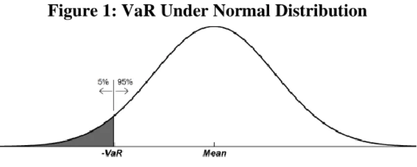
Figure 1: VaR Under Normal Distribution
Fig. 1. Representation of the left tail of the VaR under a Standard Normal Distribution where y-axis represents the density of probability and the x-axis represents the z-scores
The first parametric approach to estimate VaR was developed as part of Riskmetrics by Morgan (1996) where it assumes that the return portfolio follow a normal distribution. Under this assumption, the VaR of a portfolio at an 1 − % confidence level is calculated as:
(2) 𝑉𝑎𝑅 = 𝜇 + 𝑧𝛼𝜎
Where, is the mean of the returns, is the standard deviation of a normal distribution, 𝑧𝛼 is the value of the cumulative standardized normal distribution with α probability mass to the left. The major drawbacks of this measure developed by Riskmetrics are related to the normal distribution assumption for financial market returns. Empirical evidence shows that financial returns do not follow a normal distribution.
2.2 Volatility models
Andersen et al. (2001) affirm that asset returns share properties across a wide range of instruments, markets and time periods, known as stylized features. These stylized features include fat tails, meaning, the unconditional distribution tend to be leptokurtosis. Some of these stylized facts include: (1) volatility clustering, meaning that periods of high (low) variability tend to be followed by periods of low (high) variability; (2) leverage effect, which shows that most measures of volatility of an asset are negatively correlated with the returns of that asset itself; (3) gain/loss asymmetry meaning that stock prices and stock index values exhibit larger negative drawdowns compared to their upward movements; and finally (4) slow decay of autocorrelation in absolute returns, which translates into the autocorrelation function of absolute returns decays slowly as a function of the time lag. This last is sometimes interpreted as a sign of long-range dependence.
Several models (Abad et al. 2014) have been developed to forecast volatility, which can be broadly classified into GARCH-type models, stochastic volatility (SV) models, and, realized
(ARCH), which allows the variance to vary throughout time. This idea was further extended the model by inserting the generalized ARCH model (GARCH) represented by:
(3) 𝜎𝑡2 = 𝛼0 + 𝛼1𝑢𝑡−12 + 𝛽𝜎𝑡−12
Where σ2 represents the variance, µ2 represents the squared returns, 𝛼0 is a constant and can be interpreted as the long-run average variance, it captures long range dependence to where volatility tends to decay. The parameters (𝛼1+ 𝛽) represent the volatility clustering effect. Since then several complex models in the GARCH family have been developed that allow to capture better the volatility clustering, leverage effect, and the long-range dependence. As in the case of GARCH family, stochastic and realized volatility models have been developed in order to capture these same distribution features.
According to Abad et al. (2014) when comparing SV, GARCH family, and RV models there is mix evidence in the literature for superior predictive power and, in general, they don’t improve the results between them. The author states that it is the assumption of distribution, not the volatility models, the important factor for estimating VaR.
2.3 Accuracy test
Due to the discrepancy in the estimates produced by each VaR methodologies, it becomes essential to test the performance of VaR models. For VaR models to be accurate, they should satisfy two conditions: statistical significance when comparing the observed frequency of VaR violations w.r.t the expected one, and independence of violations (Cesarone and Colucci 2016) Virdi (2011) reviews the backtesting methods for evaluating VaR. The first of them that was developed was the unconditional coverage test developed by Kupiec (1995). The test analyzes the statistical significance of the observed frequency of violations in relation to the expected number of violations. The test can be defined as:
(4) 𝐿𝑅𝑢𝑐 = −2𝑙𝑛 ((1−𝛼)𝑇−𝑁∗𝛼𝑁
(1−𝑞)𝑇−𝛼∗𝑞𝑁)
Where α is the failure rate, T the number of observations, N the number exceptions (violations), and q is the exception rate (N/T). Under normal conditions and the Null hypothesis, the failure rate must be equal to the exception rate:
(5) 𝐻0 = 𝛼 = 𝑞
Later the independence test emerged, and it tests the independence of violations. It states that the violations should be independent through time meaning that an exception today should not depend on whether an exception occurred on the previous day. The test is defined as:
(6) 𝐿𝑅𝑖𝑛𝑑 = −2𝑙𝑛 ( (1−𝑞)𝑛00+𝑛10𝑞𝑛01𝑛11 (1−𝑞0)𝑛00𝑞0𝑛01(1−𝑞1)𝑛10𝑞1𝑛11) Where, 𝑞0 = 𝑛01 𝑛00+𝑛01 , 𝑞1 = 𝑛11 𝑛10+𝑛11 and, 𝑞 = 𝑛01+𝑛11 𝑛00+𝑛01+𝑛10+𝑛11
Then n00 means that there is not a VaR violation at time t and at t-1. n10 is: no VaR violation at time t but there is VaR violation on t-1. Next, n01 implies a VaR violation on time t but no VaR violation at time t-1 while n11 means there is a VaR violation at time t followed at other VaR violation at time t-1 (two consecutive violations).
Finally, the conditional coverage test combines the previous two with the respective equation: (7) 𝐿𝑅𝑐𝑐= 𝐿𝑅𝑢𝑐+ 𝐿𝑅𝑖𝑛𝑑
2.4 Business/Financial cycles and economic variables
Diving in the realm of economics the foundations of modern economics can be traced as far back as the various thinkers of the nineteenth century such as Adam Smith, David Ricardo, Karl Marx (Solomon 2010). Today there are several competing schools of economic thought such as the neoclassical, the post-Keynesians among others.
The Neoclassical approach is built from Walras’s General Equilibrium Theory which expounds that relative prices are determined through exchange in a competitive market by supply and demand and any individual market is necessarily in equilibrium if all other markets are also in equilibrium. Further developments culminated in the Real Business Cycle Theory also known as neoclassical synthesis, which states that fluctuations in output and employment are equilibrium phenomena and the outcome of rational economic agents responding optimally to unavoidable changes in the economic environment, with variations in the rate of technological changes being one key determinant (Cencini 2014).
One of the main representatives of post-Keynesian thought is Keen (2013a) who argues that the abstract model of the neoclassical synthesis cannot generate instability. The author states when the neoclassical synthesis is constructed, capital assets, financing arrangements that center around banks and money creation, constraints imposed by liabilities, and the problems associated with knowledge about uncertain futures are all assumed away. Keen’s analysis rises from Hyman Minsky’s innovations. The latter conceives the financial cycle as transitioning from an original state of affairs of low debt to equity ratios and high aversion to risk from the part of banks due to some recent occurrence of a systematic financial catastrophe to rising prices on par with a progressive accumulation of debt mobilized to projects and investment, ending with an overpowered aggregate demand relative to the aggregate supply and debtors having to sell their assets hastily and overcrowding the market in the process of doing so. The totality of the economy would have been driven into a halt.
Keen (2013b) shows the key indicator of impending crisis that Minsky’s hypothesis adds is the ratio of private debt to GDP, and in particular its first and second derivatives with respect to time. The ratio of debt to GDP alone is an indicator of the degree of financial stress on an economy. According to Keen (2013b) in a monetary economy in which banks endogenously create money aggregate demand is income plus the change in debt and income is primarily
expended on consumption goods. As personal consumption represents 68% of the US GDP (Bureau of Economic Analysis 2019) a variation of household consumption is the main driver for how much the GDP will vary. The above can thus be summated: a deacceleration of the total private debt will lead to a decrease in the aggregate demand and therefore to a contraction in the rate of growth of GDP which might turn negative if prolonged long enough.
There are already models with at least some capacity to predict recessions such as the Fed. This model (Federal Reserve 2019) uses the term spread of the 10-year Note and 3-month Treasury rates to calculate the probability of a recession in the United States twelve months ahead.
Beyond private debt/GDP, unemployment rate and inflation a vast number of other indicators can be used to trace the business cycle. One of them is the spread between the yield on a 10-year Treasury bond and the yield on a shorter maturity bond which Engstrom and Sharpe (2018) state as being commonly used as an indicator for predicting U.S. recessions. Bauer and Mertens (2018) give credence to this wide usage by showing that term spread has a strikingly accurate record for forecasting recessions. Periods with an inverted yield curve are reliably followed by economic slowdowns and almost always by a recession.
The Purchasing Manager's Index (PMI) is a widely watched indicator of recent U.S. economic
activity which assesses changes in production levels from month to month. It is built out of
surveys of purchasing managers at manufacturing firms by the Institute for Supply Management
(ISM). A low level together with a decrease in the PMI suggests a contraction of the
manufacturing sector. Smirnov (2011) shows that PMI gave the most drastic signal for the
economical drop in real time in December 2007.
Siegel (2016) states that the CAPE ratio is a significant variable that can predict long-run stock returns and its predictability is implied in the mean reverting feature of the CAPE ratio. The author also suggests that one of the reasons for elevated CAPE ratios is that investors are
over-optimistic about future earnings growth and when that growth does not materialize, investors will sell, sending stock prices downward. Another variable that can be used is the VIX. It is a non-economic but rather market-based measure derived from the price inputs of the S&P 500 index options and represents the market's expectation of one month forward-looking volatility.
Neffelli and Resta (2018) affirm that the VIX (CBOE volatility index) has never been such a strong fear gauge for US market than during and after the high volatility period of the 2008 financial crisis. He states that empirical evidence confirms the asymmetry response to negative returns and that even in low volatility periods, the VIX promptly reacted to market drawdowns.
3. Data and Methodology
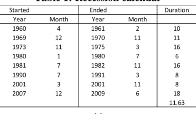
For this research it was used financial and economic data of a sample period from 01/01/1961 to 31/12/2017. To compute the daily returns, the S&P 500 stock index was downloaded using the Bloomberg-database. From the same source the monthly seasonally adjusted unemployment rate, core inflation, the ISM Manufacturing PMI, the yields from the 3-month Treasury bill and 10-year Treasury note, and the VIX were collected. The Cyclically adjusted total return price-to-earnings ratio (TRCAPE ratio) was collected from Yale resources (Yale Ressources 2019), the Total Private debt to GDP was collected quarterly from the Bank for International Settlements (International Settlements 2019), from NBER (National Bureau 2019) it was collected data referring to the business cycles (Table 1), and from New York (Federal Reserve 2019) it was downloaded monthly data of the New York Federal Reserve's probability model.
Table 1: Recession calendar
Started Ended Duration
Year Month Year Month
1960 4 1961 2 10 1969 12 1970 11 11 1973 11 1975 3 16 1980 1 1980 7 6 1981 7 1982 11 16 1990 7 1991 3 8 2001 3 2001 11 8 2007 12 2009 6 18 11.63
Although data frequency is monthly we have used every data point in that frequency except for the S&P500 volatility calculations where we used daily data because by doing so it is possible to get more information about the dispersion of the volatility. This allowed us to have a better estimation of the realized volatility when converting it into a monthly basis by summing the daily squared returns (Meddahi et al. 2011).
With the S&P500 returns we computed the average returns and volatility for three different time-frames: for its entirety, for recession periods, and for non-recession periods. This was done to discriminate the behavior of this metric among the different time-frames considered. To confirm our hypothesis, that the VaR breaks are significantly superior in periods of recession compared to periods of no recession, we tested using the Unconditional Coverage test from 01/1966 to 12/2017. For that, it was necessary to choose a volatility model that would enter as an input in the VaR estimation. The chosen criterion was the model with the lowest Mean squared error (MSE). Three models were considered to compare their MSE: the “20 days rolling window realized volatility”, the “60 days rolling window realized volatility” and the “GARCH(1,1)”. With the first two models, the 20 and the 60 days rolling window, we computed the 20 and the 60 days realized standard deviation, converted it to a monthly basis (this is done by multiplying it with the squared root of 20) for each day. After we made the average per month of that volatility. The GARCH(1,1) was estimated through standard econometrics focusing in the period from 03/1961 to 12/1965 (table 2). Among these three models, the “20 days rolling window realized volatility” was the model with the lowest value, with an MSE of 0.0004203 (table 3). However, the other models also presented similar results. After we obtained the volatility, we performed a backtest of the VaR using the “20 days rolling window realized volatility” for three different periods: (1) using all the sample from 01/1966 to 12/2017; (2) all the sample excluding recession years; and (3) all the sample excluding
recession years plus one year after and before the recessions. The purpose of the last period window presented (3) was to verify our original hypothesis while considering any S&P500 fluctuations happening before or after NBER announced either the beginning or the end of the recession.
To integrate the economic data into the adjusted VaR estimates, two strategies were considered. The first was to build an indicator able to assess with a certain degree of accuracy if there is a potential for a recession in the near future, and the second was to do a direct regression with the economic variables with the same intent.
To avoid forward looking bias, which would happen if for example the economic variable was released the 28th of a certain month but were using it as an input for a model that is making a forecast for that same month, we computed the indicator using one-month lag values of the seasonally adjusted unemployment rate, core inflation, the Manufacturing PMI, the 10y-3m yield spread, VIX, the TRCAPE ratio and the total private debt. For each one of the first six indicators we used the rank of the percentiles to understand what is the contemporary ranking of each monthly data point (mt) when compared to its historical past values starting at 01/1961 and up to period in analysis. The ranking was dynamically computed at the point mt, meaning,
for each month in the sample the indicator will only consider the ranking compared to its past values from m0to mt-1 avoiding therefore the forward looking bias. As the computation advances through time, the indicator will be able to check the relative difference in relation to the top and bottom of its historical values and therefore we were able to estimate the evolution of each indicator through the business cycle. For the core inflation and the TRCAPE ratio, in the theory, the higher it is the more it is expected that the economy is overheating, hence their ranking will be put forth in a direct proportion in the indicator. For the VIX is expected to be higher closer we are from a recession. For the yield spread, Manufacturing PMI, and Unemployment rate it is expected, as it is shown in the literature, that the lower they are, the closer the business cycle
is to the peak. As these three variables have an inverse relation with the business cycle we will use their inverse ranking as an input for the business cycle (the lower they are the higher the likelihood to enter in a recession).
To test the Keen (2013b) hypothesis that recessions tend to occur in tandem with decelerations in private debt we computed an indicator using the 1st and 2nd order derivatives of total private debt. We will thus have a dummy of value 1 when the 1st derivative of the private debt is positive and the 2nd is negative in at least the last three quarters of the last year.
Given that the VIX index only has data available since the beginning of 1990, it was necessary to estimate a proxy of the VIX for the previous years. As the VIX is derived from the price inputs of the S&P 500 index options and represents the market's expectation of one month forward-looking volatility in an annualized base (Neffelli and Resta 2018), to create a proxy to the VIX index, we tried to regress the VIX on the 20 days rolling annualized realized volatility of the S&P 500 from 01/1994 to 12/2017 with daily data to better capture the dispersion. With an R2 of 0.76 (Figure 2) the regressor seemed a good variable to build the proxy for the VIX. The proxy was then created using the 20 days rolling annualized realized volatility as an input in the regression for the data points from 01/1966 to 01/1990. The VIX indicator used as input to build the indicator for all the sample period is a combination of the actual VIX plus its proxy for the previous values it was missing.
With these seven variables set forth we can build our proprietary indicator henceforth referred to as “Market Overheating Indicator”.
To do so, we agglomerated these seven variables into one by making an equal weighted average of them. The higher the value of our proprietary, the more the economy is in a state of overheating and it's more likely that the economy enters a recession. To get an idea of how much was the relative value of the indicator at the inaugural moment of the recessions in
accordance with the NBER calendar we computed a “recession threshold” by doing the average of the value of the indicator for each point at the beginning of recessions. The Market Overheating Indicator (MOI) was further tested (table 5) to access its prediction to give correct signals of having a recession in the next 12 and 24 months after reaching the calculated “recession threshold” (61.95%). To test the robustness of the indicator and if the model was giving good results the same test was done with the New York Federal Reserve's probability model.
To assess the capability of the indicator to predict forward volatility it was computed the correlation of the indicator with the average volatility of the next 3 and 12 months. The same was done with the New York Federal Reserve's probability model.
With all this information it was time to create volatility models that incorporate the indicators presented previously. The goal of these models is to adjust the volatility upwards when there is a higher likelihood of recession given our proprietary indicators. This adjusted volatility models will serve as an input for the VaR that was than tested using the unconditional coverage test already described. We expect that the newly developed models will better capture the excess volatility in recession periods, and therefore provide better VaR estimates. Moreover, to explore the predictive power of the new adjusted volatility models it was computed for each the Mean Squared Errors with the realized volatility. Since the “20 days rolling window realized volatility” gave the lower MSE result, it will serve as a benchmark to compare the predictive power of the newly adjusted volatility models.
Model 1
For the 1st model the adjusted realized volatility was regressed for the subsample period of 01/2004 to 12/2017 taking into account all the economic and financial variables used until now:
(8) 𝐴𝑑𝑗_𝑟𝑒𝑎𝑙𝑖𝑧𝑒𝑑_𝑣𝑜𝑙𝑎𝑡𝑖𝑙𝑡𝑦𝑡= + 1𝑈𝑛𝑝𝑡−1+2𝐼𝑛𝑓𝑡−1+3𝑃𝑀𝐼𝑡−1+4𝐶𝐴𝑃𝐸𝑡−1+5𝑌_𝑠𝑝𝑟𝑒𝑎𝑑𝑡−1+6𝑃𝑟𝑖𝑣_𝑑𝑒𝑏𝑡𝑡−1+7𝑉𝐼𝑋𝑡−1+
𝜀𝑡
In the first model there were some insignificant variables (table 10), so we remade the model by taking them out:
(9) 𝐴𝑑𝑗_𝑟𝑒𝑎𝑙𝑖𝑧𝑒𝑑_𝑣𝑜𝑙𝑎𝑡𝑖𝑙𝑡𝑦𝑡= + +1𝑃𝑀𝐼𝑡−1+2𝑃𝑟𝑖𝑣_𝑑𝑒𝑏𝑡𝑡−1+3𝑉𝐼𝑋𝑡−1+ 𝜀𝑡
Model 2
For the 2nd model the adjusted realized volatility was regressed for the subsample period of 01/2004 to 12/2017 using the following equation:
(10) 𝐴𝑑𝑗_𝑟𝑒𝑎𝑙𝑖𝑧𝑒𝑑_𝑣𝑜𝑙𝑎𝑡𝑖𝑙𝑡𝑦𝑡= + +120𝑑_𝑟𝑚𝑣𝑡−1+2𝑂𝑣𝑒𝑟ℎ𝑒𝑎𝑡𝑖𝑛𝑔 𝐼𝑛𝑑𝑖𝑐𝑎𝑡𝑜𝑟𝑡−1+ 𝜀𝑡
Model 3
For the 3rd model the adjusted realized volatility was computed simply by adding the excess volatility of 2.37% (which is the difference between the volatility in recessions compared to no recessions periods) for the next 18 months each time the indicator is above the dynamic indicator threshold (61.95%). Those 18 months correspond to the average length of a recession that lasts 12 months (table 1) in our sample plus 6 months that is the average length it takes to enter in a recession after that MOI has given a correct signal (table 5).
Model 4
The 4th model is similar to Model 2 but the indicator was subdivided in percentiles to take into account the excess volatility for each interval. The intent of this subdivision it to capture not only the excess of volatility when the indicator is high but also to capture the lack of volatility for the periods when the indicator is low.
As the 4th model was excessively underestimating volatility when the indicator was below 50%, a 2nd version of the 4th model was created, named Model 5, by taking only into account the
4. Results
By analyzing the behavior of the returns and volatility for the different subperiods we discovered that the average monthly returns are almost symmetrical in periods of recessions and periods excluding recessions, -0.75% and 0.76% respectively (table 4). As to the volatility, the results were more interesting. With an average monthly volatility of 4.32% for all the sample, we obtained 6.24% in recessions and 3.88% for all the sample excluding recessions. The difference between the two periods is the excess volatility of 2.37%. These results are very interesting because they show a clear discrepancy of the standard deviation when they are sorted by recessions and periods of expansion. This tells us that the volatility is nonrandom and not independent through time, since we were able to identify two periods where the volatility has a consistently different behavior and we did this by demonstrating excess volatility in periods of recessions.
After, to test the statistical significance of VaR breaks and the independence of the violations. We backtested the VaR for the sample period and two sub sample periods. The following tables show the number of observations (T), the exception rate (N/T) that is the number of violations over the total observations, the tests and it respective critical values for the different significance levels. We could observe the following results:
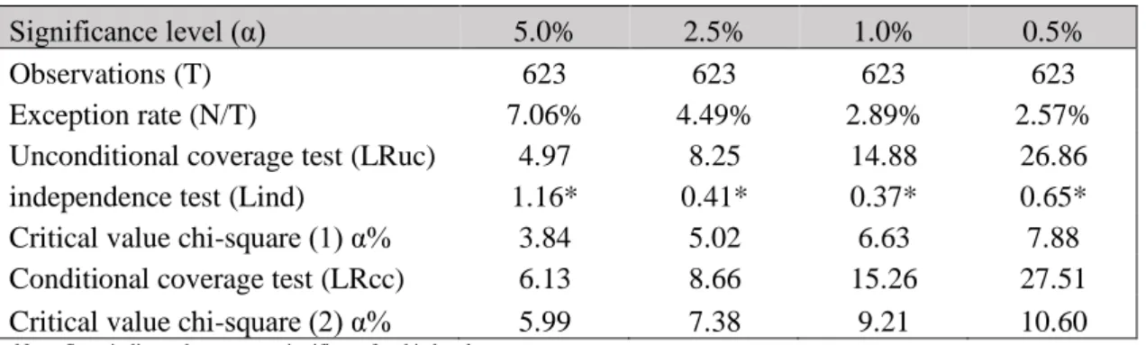
Table 7: VaR backtest outcomes for all the sample
Significance level (α) 5.0% 2.5% 1.0% 0.5%
Observations (T) 623 623 623 623
Exception rate (N/T) 7.06% 4.49% 2.89% 2.57%
Unconditional coverage test (LRuc) 4.97 8.25 14.88 26.86 independence test (Lind) 1.16* 0.41* 0.37* 0.65* Critical value chi-square (1) α% 3.84 5.02 6.63 7.88 Conditional coverage test (LRcc) 6.13 8.66 15.26 27.51 Critical value chi-square (2) α% 5.99 7.38 9.21 10.60
In the period containing all the data available the unconditional coverage test demonstrates that the VaR was rejected for all significance levels. Then, the number of violations is significantly higher than it should be and therefore, without adjusting volatility, the VaR is underestimating the potential risk. This proves VaR is not an accurate risk measure, as previously hypothesized. At this point our first objective has been achieved. We have given grounding to Dalio ́s statements about the inaccuracy of VaR in respect to the subprime crisis.
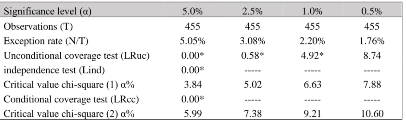
Table 8: VaR backtest outcomes for all the sample excluding recession years
Significance level (α) 5.0% 2.5% 1.0% 0.5%
Observations (T) 455 455 455 455
Exception rate (N/T) 5.05% 3.08% 2.20% 1.76%
Unconditional coverage test (LRuc) 0.00* 0.58* 4.92* 8.74
independence test (Lind) 0.00* --- --- ---
Critical value chi-square (1) α% 3.84 5.02 6.63 7.88 Conditional coverage test (LRcc) 0.00* --- --- --- Critical value chi-square (2) α% 5.99 7.38 9.21 10.60
Note: Stars indicate the test was significant for this level and (---) indicates the test was not applicable
If the recession periods are excluded, the Unconditional coverage test shows a more effective VaR model. The test shows significant results at significance levels of 5%, 2.5%, and 1%. That means our VaR provides fairly accurate measures of true risk.
Table 9: VaR backtest outcomes for all the sample excluding recession years plus year after and before
Significance level (α) 5.0% 2.5% 1.0% 0.5%
Observations (T) 311 311 311 311
Exception rate (N/T) 6.11% 3.54% 2.25% 1.93%
Unconditional coverage test (LRuc) 0.75* 1.22* 3.63* 7.38* independence test (Lind) --- --- --- --- Critical value chi-square (1) α% 3.84 5.02 6.63 7.88 Conditional coverage test (LRcc) --- --- --- --- Critical value chi-square (2) α% 5.99 7.38 9.21 10.60
Similar results for the Unconditional coverage test were obtained by removing the recessions years plus one year before and after but here they are also significant at the significance level of 0.5%.
These results are important because they demonstrate that VaR breaks occur much more often in periods of recessions that it was supposed to. This demonstrates that the left fat tail is concentrated in the years of recessions and therefore the risk in recessions is being underestimated. Then, if it is possible to adjust the VaR for the periods one knows are going to be more volatile, one can get a better estimation of risk during all the periods of the sample, regardless of the economic conditions.
After computing the Market Overheating Indicator, we tested its predictive power to sense a recession for 1 year and 2 years following the indicator having reached the recession threshold. For 12 months (1 year) it gave 7/7 correct signals, predicting all the recessions in the sample, and 6 false signals with an accuracy of 53.85%. For 24 months (2 years) the accuracy increased to 70% (table 5). With the New York Federal Reserve's probability model, we got the same results for 12 months but for 24 months the accuracy decreased to 63.64% compared to the Market overheating indicator (table 6).
To assess the capability of the indicator to predict forward volatility it was analyzed the correlation of forward 1-year volatility (Figure 4) with the Market overheating indicator and the Fed probability model indicator. The results obtained were 37.1% and 24.54% respectively. This indicates that the Market overheating indicator has a good potential to predict forward excess volatility and, by consequence, forward risk. These results meant that our proprietary indicator is indeed quite accurate and a good proxy to access the overheating of the economy and to predict recessions.
The following tables contain the backtest results of the unconditional coverage test and Mean squared errors for the different volatility models shown previously. The Mean squared error of the adjusted volatility of each model is represented as MSE ((adj_v)-rv) and MSE (20d_mrv-rv) for the 20 days rolling window realized volatility. In this table there are two variables that are important: The unconditional coverage test and the Mean squared error of the adjusted volatility of each model. The first refers to the performance of the VaR by testing if it is measuring the number of violations correctly. The second refers to the predictive power of the volatility model considered. The goal is to obtain in the Unconditional Coverage test a well performing VaR without distorting too much the predictive power of the volatility. In other words, to get a model that doesn’t reject the VaR for the maximum number of significance levels possible and also has the lowest possible MSE.
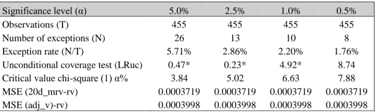
Table 12: VaR backtest outcomes for Model 1
Significance level (α) 5.0% 2.5% 1.0% 0.5%
Observations (T) 455 455 455 455
Number of exceptions (N) 26 13 10 8
Exception rate (N/T) 5.71% 2.86% 2.20% 1.76%
Unconditional coverage test (LRuc) 0.47* 0.23* 4.92* 8.74 Critical value chi-square (1) α% 3.84 5.02 6.63 7.88 MSE (20d_mrv-rv) 0.0003719 0.0003719 0.0003719 0.0003719 MSE (adj_v)-rv) 0.0003998 0.0003998 0.0003998 0.0003998
Note: Stars indicate the test was significant for this level
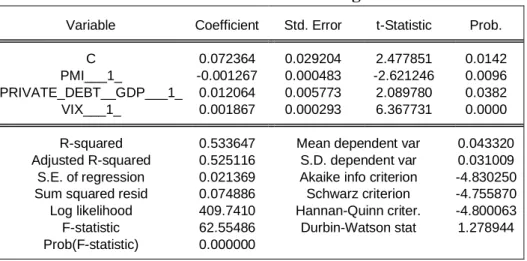
Model 1 (table 10&11) was a surprise because it doesn’t reject the VaR for the various significance levels (5%, 2.5%, and 1%) without sacrificing too much the MSE, meaning that the predictive power of the this new volatility isn’t lost compared to the volatility benchmark (20 days rolling window realized volatility). It is important to consider that the VIX proxy was built by a regression with realized volatility, hence, Model 1 has the past realized volatility implied in an indirect fashion. With p-values of 0.0096 and 0.0382 (Table 11) for the PMI and private debt, respectively, the variables are significant at a 5% significance level. This
demonstrates that the variables are doing a good job capturing the variation in the business cycles.
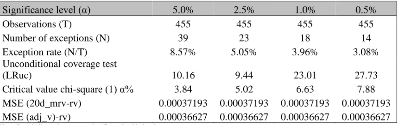
Table 13: VaR backtest outcomes for Model 2
Significance level (α) 5.0% 2.5% 1.0% 0.5%
Observations (T) 455 455 455 455
Number of exceptions (N) 39 23 18 14
Exception rate (N/T) 8.57% 5.05% 3.96% 3.08%
Unconditional coverage test
(LRuc) 10.16 9.44 23.01 27.73
Critical value chi-square (1) α% 3.84 5.02 6.63 7.88 MSE (20d_mrv-rv) 0.00037193 0.00037193 0.00037193 0.00037193 MSE (adj_v)-rv) 0.00036627 0.00036627 0.00036627 0.00036627
Note: Stars indicate the test was significant for this level
Model 2, with the lowest MSE ((adj_v)-rv), is the only one to have a superior predictive power compared to the volatility benchmark. Nevertheless, it does a very poor job to capture the violations of the VaR since the Unconditional Coverage test was rejected for all the significance levels considered.
Table 14: VaR backtest outcomes for Model 3
Significance level (α) 5.0% 2.5% 1.0% 0.5%
Observations (T) 623 623 623 623
Number of exceptions (N) 30 19 11 8
Exception rate (N/T) 4.82% 3.05% 1.77% 1.28%
Unconditional coverage test (LRuc) 0.05* 0.72* 3.00* 5.36* Critical value chi-square (1) α% 3.84 5.02 6.63 7.88 MSE (20d_mrv-rv) 0.0004203 0.0004203 0.0004203 0.0004203 MSE (adj_v)-rv) 0.0005623 0.0005623 0.0005623 0.0005623
Note: Stars indicate the test was significant for this level
Model 3 was constructed in order to integrate the excess volatility by summing it to the realized volatility of the data point each time the indicator was above the recession threshold and staying adjusted for the next 18 months. This model was the best performer in terms of adjusting the VaR and it stayed significant even for a significance of 0.5% however, with the highest MSE ((adj_v)-rv), it was the worst to predict volatility accurately. These results signal us that when the indicator gives a false signal (we had a signal but the recession hadn’t occurred), the model
is overestimating largely the volatility in those periods as patent in the MSE. Even if the predictive power of the volatility stays short of optimal it is nevertheless a good model due to its high performance in adjusting the VaR.
Table 15: VaR backtest outcomes for Model 4
Significance level (α) 5.0% 2.5% 1.0% 0.5%
Observations (T) 623 623 623 623
Number of exceptions (N) 60 42 31 22
Exception rate (N/T) 9.63% 6.74% 4.98% 3.53%
Unconditional coverage test (LRuc) 22.39 31.64 50.95 48.82 Critical value chi-square (1) α% 3.84 5.02 6.63 7.88 MSE (20d_mrv-rv) 0.0004203 0.0004203 0.0004203 0.0004203 MSE (adj_v)-rv) 0.0005010 0.0005010 0.0005010 0.0005010
Note: Stars indicate the test was significant for this level
The goal with Model 4 was to add and subtract the excess volatility depending on the state of the economy. To do this we broke the indicator by range of percentiles to know the excess of volatility that came up on those ranges. The results are presented in table 17. As it can be observed, on average, the higher the Market Overheating Indicator the bigger the average excess volatility. It also shows that for values below 50% the excess volatility tends to be negative. This is in line with our expectations.
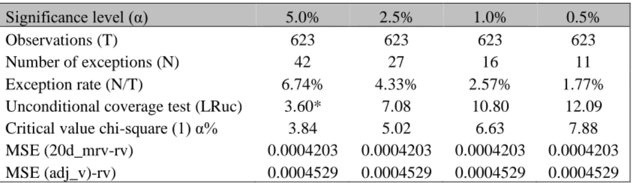
Table 16: VaR backtest outcomes for Model 5
Significance level (α) 5.0% 2.5% 1.0% 0.5%
Observations (T) 623 623 623 623
Number of exceptions (N) 42 27 16 11
Exception rate (N/T) 6.74% 4.33% 2.57% 1.77%
Unconditional coverage test (LRuc) 3.60* 7.08 10.80 12.09 Critical value chi-square (1) α% 3.84 5.02 6.63 7.88 MSE (20d_mrv-rv) 0.0004203 0.0004203 0.0004203 0.0004203 MSE (adj_v)-rv) 0.0004529 0.0004529 0.0004529 0.0004529
Note: Stars indicate the test was significant for this level
The results from Model 4 were not optimal so Model 5 was created by removing the percentiles adjustment below 50, to test if the model is removing too much excess volatility for the lower percentile ranges. The Unconditional coverage test and the MSE ((adj_v)-rv) of 2nd version of
the Model 4 gave much better results than the previous one with a reasonable VaR fitting and a MSE not far from the benchmark volatility.
As our goal was to get a model that doesn’t reject the VaR for the maximum number of significance levels possible and, at the same time, also has the lowest possible MSE for the adjusted volatility. Some models proved themselves to be up to the task. The results of Model 1, Model 3 and the Model 5 display a fine balance between both.
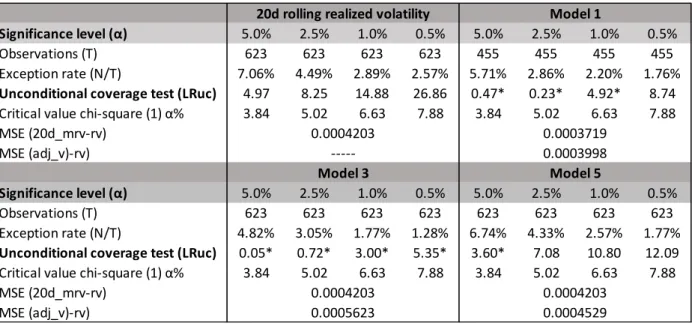
The table below contains the summary of the main statistics of the last three models compared to the 20 days rolling realized volatility. The Unconditional coverage test shows that volatility models that were adjusted for business cycles (Model 1, Model 3, and Model 5) demonstrate by far superior results when compared to the one where it was not adjusted (20 days rolling realized volatility). We conclude that by adjusting the volatility to business and financial cycles it is possible to get a more performant VaR.
Table 18: Comparison of the VaR backtest outcomes with and without adjustment to the business cycle
Note: Stars indicate the test was significant for this level
Significance level (α) 5.0% 2.5% 1.0% 0.5% 5.0% 2.5% 1.0% 0.5%
Observations (T) 623 623 623 623 455 455 455 455
Exception rate (N/T) 7.06% 4.49% 2.89% 2.57% 5.71% 2.86% 2.20% 1.76%
Unconditional coverage test (LRuc) 4.97 8.25 14.88 26.86 0.47* 0.23* 4.92* 8.74
Critical value chi-square (1) α% 3.84 5.02 6.63 7.88 3.84 5.02 6.63 7.88
MSE (20d_mrv-rv) MSE (adj_v)-rv)
Significance level (α) 5.0% 2.5% 1.0% 0.5% 5.0% 2.5% 1.0% 0.5%
Observations (T) 623 623 623 623 623 623 623 623
Exception rate (N/T) 4.82% 3.05% 1.77% 1.28% 6.74% 4.33% 2.57% 1.77%
Unconditional coverage test (LRuc) 0.05* 0.72* 3.00* 5.35* 3.60* 7.08 10.80 12.09
Critical value chi-square (1) α% 3.84 5.02 6.63 7.88 3.84 5.02 6.63 7.88
MSE (20d_mrv-rv) MSE (adj_v)-rv) 0.0004203 0.0004203 0.0004203 0.0003719 Model 1 ---Model 3 0.0003998 Model 5 0.0005623 0.0004529
5. Conclusion
We examined the hypothesis that the number of violations happening in periods of recessions were the main factor that makes the parametric VaR model was being rejected. It was observed by backtest that the VaR exception rate was significantly reduced when the periods of recession were removed giving a clue that the fat tail feature of returns can be concentrated in the periods of recessions. We uncover that there is a substantial excess volatility in periods of recessions and with this information and the backtest concluded that the volatility needed to be adjusted for periods of recessions as it was not incorporating accurately the risk for that periods. To do this we created an indicator to assess the state of the economy in function of some economic and financial indicators. We then estimate four different volatility models with all of them incorporating business and financial cycles features to be used as input for VaR. Model 1, Model 3, and the Model 5 proved themselves robust enough to estimate the VaR. However, these models are not perfect and have a lot of room to be further improved in the future. The MOI was put in contrast with the New York Federal Reserve's probability model and was able to produce less false recession signals and have a better correlation with the 1-year forward volatility of 37.1% vs 24.54%.
This study considered just the American economy. To get more robust results we could have used data from other economies as well. The fulcrum of this paper springs out of the economic and financial indicators presented. There could be other indicators, better suited to predict recessions than the ones considered. To test the VaR it was only used the S&P500, other index or asset classes could have been used. Lastly, there are other volatility models, not used here, more capable of seizing upon the stylized features of returns.
We consider these results to have potential to be the basis for further research. For example, by accessing the fragility of the economy it may be possible to be one step ahead prepared for
future volatility. We hope that the research on this topic will help banks, investors, and financial institutions to be more prepared for future recessions and adjust leverage and the portfolio weights according to intrinsically state of the economy. We also hope that this paper will incentivize further research in the methods to evaluate risk.
6. References
Abad P, Benito S, López C (2014) A comprehensive review of Value at Risk methodologies. Spanish Rev Financ Econ 12:15–32. https://doi.org/10.1016/j.srfe.2013.06.001
Andersen TG, Bollerslev T, Diebold FX, Ebens H (2001) The distribution of realized stock return volatility
Basle C (1996) The amendment to the capital accord to incorporate market risk
Bauer MD, Mertens TM (2018) Economic Forecasts with the Yield Curve. FRBSF Econ Lett 2018–07:1–5
Bureau of Economic Analysis U. Shares of gross domestic product: Personal consumption expenditures (DPCERE1Q156NBEA) | FRED | St. Louis Fed.
https://fred.stlouisfed.org/series/DPCERE1Q156NBEA. Accessed 9 Dec 2019 Cencini A (2014) Neoclassical , New Classical and New Business Cycle Economics : A
Critical
Cesarone F, Colucci S (2016) A quick tool to forecast value-at-risk using implied and realized volatilities. J Risk Model Valid 10:71–101. https://doi.org/10.21314/JRMV.2016.163 Dalio RAY (2018) A Template For Understanding Big Debt Crises. Greenleaf Book Group,
Austin, TX
Engle (1982) Autoregressive Conditional Heteroscedacity with Estimates of variance of United Kingdom Inflation,journal of Econometrica, Volume 50, Issue 4 (Jul.,
1982),987-1008. Econometrica 50:987–1008
Engle RF, Manganelli S (2004) CAViaR: Conditional autoregressive value at risk by regression quantiles. J Bus Econ Stat 22:367–381.
https://doi.org/10.1198/073500104000000370
Engstrom E, Sharpe S (2018) The Near-Term Forward Yield Spread as a Leading Indicator: A Less Distorted Mirror. Financ Econ Discuss Ser 2018:.
https://doi.org/10.17016/feds.2018.055
Federal Reserve NY Federal Reserve Bank of New York, The Yield Curve as a Leading Indicator. https://www.newyorkfed.org/research/capital_markets/ycfaq.html
International Settlements B for Credit to the non-financial sector. https://www.bis.org/statistics/totcredit.htm. Accessed 10 Oct 2019
Jorion P (2006) Value at Risk: The New Benchmark for Managing Financial Risk, 3rd edn. McGraw-Hill Education - Europe, New York
Keen S (2013a) A monetary Minsky model of the Great Moderation and the Great Recession. J Econ Behav Organ 86:221–235. https://doi.org/10.1016/j.jebo.2011.01.010
Keen S (2013b) Predicting the “Global Financial Crisis”: Post-Keynesian Macroeconomics. Econ Rec 89:228–254. https://doi.org/10.1111/1475-4932.12016
Kupiec P (1995) Techniques for verifying the accuracy of risk measurement models. J Deriv 2:73–84
Meddahi N, Mykland P, Shephard N (2011) Realized volatility. J Econom 160:1. https://doi.org/10.1016/j.jeconom.2010.07.005
Morgan (1996) RiskMetricsTM—Technical Document
https://www.nber.org/cycles/cyclesmain.html. Accessed 10 Oct 2019
Neffelli M, Resta MR (2018) Is VIX Still the Investor Fear Gauge? Evidence for the US and BRIC Markets. SSRN Electron J 1–29. https://doi.org/10.2139/ssrn.3199634
Siegel JJ (2016) The Shiller CAPE Ratio: A New Look. 3312:. https://doi.org/10.2469/faj.v72.n3.1
Smirnov S (2011) THOSE UNPREDICTABLE RECESSIONS … BASIC RESEARCH PROGRAM. 1–24
Solomon MS (2010) Critical Ideas in Times of Crisis : Reconsidering Smith , Marx , Keynes , and Hayek. 7731:. https://doi.org/10.1080/14747731003593356
Virdi NK (2011) A Review of Backtesting Methods for Evaluating Value-at- Risk. Int Rev Bus Res 7:14–24
Yale Ressources I ONLINE DATA ROBERT SHILLER.
7. Appendix
Table 2: Estimation of the GARCH parameters
Table 3: Mean squared errors of volatility models
Table 4: SPX statistics
average returns 0.54%
average monthly volatility 4.32% avg returns in recession -0.75% volatility in recession 6.24%
avg returns excluding recessions 0.76% volatility excluding recessions 3.88% excess volatility in recession 2.37%
Table 5: Market overheating summary rmv 20d rmv 60d garch (1,1) MSE 0.0004203 0.0004423 0.0004266 N. of months 12 24 Total signals 13 10 False signals 6 3 Correct signals 7 7 N. Of recessions 7 7 Recessions predicted 7 7 Recessions missed 0 0 Accuracy 53.85% 70.00%
Conditional probability of signal if recession 100% 100.00% Average number of months it takes to enter
5.71 7.29
GARCH = C(3) + C(4)*RESID(-1)^2 + C(5)*GARCH(-1)
Variable Coefficient Std. Error z-Statistic Prob.
C 0.000627 0.000138 4.535240 0.0000 AR(1) 0.169337 0.028615 5.917824 0.0000 Variance Equation C 1.16E-06 2.03E-07 5.722808 0.0000 RESID(-1)^2 0.204038 0.017313 11.78503 0.0000 GARCH(-1) 0.772310 0.016903 45.69161 0.0000
R-squared 0.015162 Mean dependent var 0.000207
Adjusted R-squared 0.014532 S.D. dependent var 0.006336 S.E. of regression 0.006290 Akaike info criterion -7.772564 Sum squared resid 0.061843 Schwarz criterion -7.755453 Log likelihood 6087.031 Hannan-Quinn criter. -7.766203 Durbin-Watson stat 2.053412
Table 6: New York Federal Reserve's probability model summary
Table 10: Model 1 regression
Table 11: Model 1 2nd version regression
Variable Coefficient Std. Error t-Statistic Prob.
C 0.072364 0.029204 2.477851 0.0142
PMI___1_ -0.001267 0.000483 -2.621246 0.0096
PRIVATE_DEBT__GDP___1_ 0.012064 0.005773 2.089780 0.0382
VIX___1_ 0.001867 0.000293 6.367731 0.0000
R-squared 0.533647 Mean dependent var 0.043320
Adjusted R-squared 0.525116 S.D. dependent var 0.031009 S.E. of regression 0.021369 Akaike info criterion -4.830250 Sum squared resid 0.074886 Schwarz criterion -4.755870 Log likelihood 409.7410 Hannan-Quinn criter. -4.800063 F-statistic 62.55486 Durbin-Watson stat 1.278944 Prob(F-statistic) 0.000000 N. of months 12 24 Total signals 13 11 False signals 6 4 Correct signals 7 7 N. Of recessions 7 7 Recessions predicted 7 7 Recessions missed 0 0 Accuracy 53.85% 63.64%
Conditional probability of signal if recession 100% 100.00% Average number of months it takes to enter
recession after giving a correct signal 4.57 5.29
Variable Coefficient Std. Error t-Statistic Prob.
C 0.031242 0.054561 0.572618 0.5677 UNEMPLOYMENT_RATE___1_ 0.001291 0.002947 0.438017 0.6620 PMI___1_ -0.002026 0.000760 -2.663841 0.0085 CAPE_RATIO___1_ 0.002389 0.001988 1.201566 0.2313 YIELD_SPREAD_3M10Y___1_ 0.002331 0.002479 0.940132 0.3486 PRIVATE_DEBT__GDP___1_ 0.016505 0.007828 2.108429 0.0365 VIX___1_ 0.002111 0.000388 5.434467 0.0000
R-squared 0.546204 Mean dependent var 0.043320
Adjusted R-squared 0.529292 S.D. dependent var 0.031009 S.E. of regression 0.021275 Akaike info criterion -4.821831 Sum squared resid 0.072870 Schwarz criterion -4.691666 Log likelihood 412.0338 Hannan-Quinn criter. -4.769004
F-statistic 32.29743 Durbin-Watson stat 1.273003
Table 17: Excess volatility by range of percentiles
Figure 2: VIX regressed on 20d rolling annualized realized volatility
Fig. 2. Figure 2 shows the regression of the VIX with “20d rolling annual realized volatility”
Figure 3: Market overheating indicator
Fig. 3. The change of the Market overheating indicator through time range average volatility excess volatility
[0:25] 2.39% -1.94% [25:30] 3.35% -0.98% [30:35] 3.25% -1.07% [35:40] 4.39% 0.06% [40:45] 4.24% -0.08% [45:50] 3.63% -0.69% [50:55] 3.75% -0.58% [55:60] 5.49% 1.16% [60:65] 4.57% 0.25% [65:70] 4.69% 0.37% [70:75] 6.99% 2.67% [75:100] 5.92% 1.59% y = 74.001x + 8.0363 R² = 0.7561 0 20 40 60 80 100 0.00% 20.00% 40.00% 60.00% 80.00% 100.00% V IX
20d rolling annualized realized volatility
0.00% 10.00% 20.00% 30.00% 40.00% 50.00% 60.00% 70.00% 80.00% 90.00% 1/ 1 96 6 5/ 1 96 8 9/ 1 97 0 1/ 1 97 3 5/ 1 97 5 9/ 1 97 7 1/ 1 98 0 5/ 19 82 9/ 1 98 4 1/ 1 98 7 5/ 1 98 9 9/ 1 99 1 1/ 1 99 4 5/ 1 99 6 9/ 1 99 8 1/ 2 00 1 5/ 20 03 9/ 2 00 5 1/ 2 00 8 5/ 2 01 0 9/ 2 01 2 1/ 2 01 5 5/ 2 01 7 P ER CE NT YEARS
Figure 4: Indicator correlation with forward volatility
Fig. 4. This figure shows the indicator with and forward volatility. When putting together it shows an apparent correlation between them
Figure 5: Fed probability model vs Market Overheating Indicator
Fig. 5. This figure compares the fed probability model with the Market Overheating Indicator
0 0.05 0.1 0.15 0.2 0.25 0.00% 20.00% 40.00% 60.00% 80.00% 100.00% 1/ 1/ 19 66 12 /1 /1 96 8 11 /1 /1 97 1 10 /1 /1 97 4 9/ 1/ 19 77 8/ 1/ 19 80 7/ 1/ 19 83 6/ 1/ 19 86 5/ 1/ 19 89 4/ 1/ 19 92 3/ 1/ 19 95 2/ 1/ 19 98 1/ 1/ 20 01 12 /1 /2 00 3 11 /1 /2 00 6 10 /1 /2 00 9 9/ 1/ 20 12 8/ 1/ 20 15 Indicator
rolling window 3m volatility
Forward looking 12m rolling volatility
0.00% 10.00% 20.00% 30.00% 40.00% 50.00% 60.00% 70.00% 80.00% 90.00% 0.00% 20.00% 40.00% 60.00% 80.00% 100.00% 120.00% 1 /1 9 6 6 12 /1 96 8 11 /1 97 1 10 /1 97 4 9 /1 9 7 7 8 /1 9 8 0 7 /1 9 8 3 6 /1 9 8 6 5 /1 9 8 9 4 /1 9 9 2 3 /1 9 9 5 2 /1 9 9 8 1 /2 0 0 1 12 /2 00 3 11 /2 00 6 10 /2 00 9 9 /2 0 1 2 8 /2 0 1 5