A Model Updating Method for Plate Elements Using Particle Swarm
Optimization (PSO), Modeling the Boundary Flexibility, Including
Un-certainties on Material and Dimensional Properties
Abstract
It is a well-known fact that, in a real engineering situation, fixtures are not ideally stiff, so numerical simulations using them are unlikely to present re-sults that are consistent with the experimental ones. The present paper in-tends to describe a model updating methodology inserting translational and rotational springs in order to better represent the real clamping. For that purpose, the PSO stochastic optimization method will be used to determine the spring stiffness in an iterative way. In addition, uncertainties regarding the material properties, such as density and Young’s Modulus, as well as workpiece dimensions, will also be taken into account in the optimization algorithm. Once the experimental natural frequencies and the geometry of the studied parts are known, the algorithm automatically updates the model, approximating the natural frequencies obtained from the numerical model to the experimentally obtained ones as closely as possible. In addition, the modal shapes of the updated simulation will be compared to the experi-mental data and to a rigid boundary simulation. Results will demonstrate that the proposed methodology efficiently represents the fixturing flexibil-ity: both natural frequencies and mode shapes found were close to the real dynamic system.
Keywords
Model Updating; Modal Analysis; Fixturing System; Optimization; Mode Shape.
1 INTRODUCTION
The boundary conditions are an important issue regarding any numerical or experimental engineering prob-lem. To solve a real problem, a model is created, simplifying it by making hypotheses and assumptions. However, some assumptions are occasionally weak or ultimately not true, such as the clamping of a workpiece in a fixture system, in which the stiffness is considered infinite. Some discrepancies between the model and the real situation are originated from structural geometry differences, material properties and inaccurate boundary conditions (Jai-shi & Ren, 2007). Hence, the finite element model is not able to accurately predict the dynamic responses of struc-tures and the model must be updated (Sehgal and Kumar 2016).
The model updating method is a strong tool to adjust the model to the empirical results. Basically, it changes some parameters of the numerical or analytical model to match the experimental data. In this regard, Kabe (1984) used the model updating technique to adjust a mass-spring system, changing the stiffness matrix directly to ap-proximate the simulated natural frequencies to the experimental ones. Using a finite element model, Mottershead et al. (1996) applied the model updating method to properly model a welded joint on a plate, once the plate support had some flexibility. To achieve the flexibility of the practical experiment, the chosen updating parameter was the effective length of the plate.
Ahmadian et al. (1998) performed a study on a frame structure where the joints were the major source of discrepancies between the model and the test results. The beam elements’ stiffness was updated to adjust the model’s natural frequencies. Zhang et al. (2014) also used the model updating technique to adjust the deflection of a truss. The stiffness of the joints was determined as the correction factors and the deflection of the updated model, applying stepwise uniform design, was compared to the experimental data. Jaishi & Ren (2007) applied a multi-objective optimization technique, using model updating to adjust eigenvalue and strain energy residuals. The first
Doglas Negria*
Felipe Klein Fiorentina
Joel Martins Crichigno Filhoa
a Departamento de Engenharia Mecânica,
Uni-versidade do Estado de Santa Catarina – UDESC, Joinville, Santa Catarina, Brasil. E-mail: [email protected], [email protected], [email protected].
*Corresponding author
http://dx.doi.org/10.1590/1679-78254342
ten natural frequencies were adjusted using a finite beam element model to fit the experimental ones and, in addi-tion, the natural modes obtained from the updated model were compared to the experimental data.
Those two model updating techniques can be classified as non-iterative and iterative. The first one directly updates the mass and stiffness matrices and, as a model updating method, the computationally obtained parame-ters tend to coincide with the real ones (Berman and Nagy, 1983), but they are usually not physically meaningful, once the structural connectivity and parameters are not maintained (Baruch and Bar Itzhack, 1978). The second one (iterative method) consists on solutions from several loops, and usually needs optimization formulations. Er-rors between numerical and experimental data are set as an objective function, and a pre-selected set of physical parameters are changed to minimize it (Friswell and Mottershead, 2013). The iterative model updating is the most common and robust method, since when the correct optimization parameters and methods are chosen the solution tends to maintain its physical foundation and achieve acceptable correlations.
A problem arises because of the non-linear relationship between the vibration data and the physical parame-ters, making the solution more complex (Bussetta et al., 2017). To overcome such problem, the application of the Particle Swarm Optimization (PSO) has been growing in recent years. The PSO is based on the artificial intelligence evolutionary algorithm proposed by (Eberchart and Kennedy, 1995), inspired by the observation of birds flocking and searching for food, which represents a form of social intelligence. This technique is easy to implement and suited for many different classes of problems, such as optimum structural design (Plevris and Papadrakakis, 2011), structural damage detection (Seyedpoor 2012), parameter identification (Galewski, 2016) and finite element up-dating (Moradi et al. 2010). Marwala (2007), applying PSO in FE model upup-dating, observed that the updated natural frequencies and modal shapes were more accurate and faster than using simulated annealing and genetic algo-rithms.
The object of this study is a cantilever plate, clamped at a fixture system. An efficient fixturing system must be very rigid, hold the workpiece in place and accurately maintain a precise position (Boyle et al., 2011).
Since the real fixation system is far from being rigid, the workpiece can translate and rotate at the interface. Hence, rotational and translational springs can be applied to the boundary to approximate the real physical situa-tion. The stiffness of two springs were chosen to be the updating parameters for the optimization model. Choosing the right updating parameters is one of the most important steps, once they have to maintain the model’s physical significance. If other parameters were selected, such as the element’s stiffness, the model’s natural frequencies would probably converge to the experimental ones, but the model would not properly represent the physical phe-nomenon.
This paper focuses on the problem of a rigid clamping system hypothesis and how the model updating method may approximate the numerical model to the real system. The simulations were performed using plate elements. Three approaches are taken. The first one consists in updating the translational and rotational spring’s stiffness. In the second updating procedure, the material properties (Young’s modulus and density) are included as parameters to be optimized. Workpiece dimensions (free length, width and thickness) are added at the last simulation. For the optimization method, the Particle Swarm Optimization (PSO) is applied (Eberchart and Kennedy, 1995). The main reasons for this decision is that the method has an easy implementation and because of the non-linear relationship between the vibration data and the physical parameters (Jaishi and Ren, 2007).
The updated model’s natural frequencies and mode shapes are compared to the experimental data and to a model using a rigid boundary condition. This work aims to show how the hypothesis of a zero-displacement bound-ary may not be a reasonable consideration, and how model updating can improve the numerical formulation. Also, this study investigates which design parameters are more suitable to describe the workpiece’s dynamics. An impact hammer modal test is performed on a clamped plate, and the first four natural frequencies are obtained. In addition, the frequency responses are measured at a single point, while several points were impacted along the plate. Such procedure is performed in order to construct the modal shape of the experimental data.
To evaluate how close the experimental modal shapes are to the adjusted ones, the Modal Assurance Criterion (MAC), which basically correlates two modal shapes to a scalar number, is calculated. If both modes are strongly related, the MAC number is close to one. If both modes are non-related, it is close to zero (Allemang and Brown, 1982).
1.1 Originality of this Work
tolerances of the workpiece. The optimization routines focus on the eigenvalues problem, but the modal shape of the optimized models are evaluated too.
1.2 Outline
The present work is composed of 6 sections, the first being related to the performed experimental analysis, followed by the finite element model (section 3). In sequence, a model updating method is proposed, using three different approaches. The following section explains the optimization process used for this paper (section 5). After those formulations, the results are presented and discussed (section 6). Finally, some observations and final re-marks are elucidated in the ‘conclusions’ section.
2 EXPERIMENTAL ANALYSIS
In practical engineering situations, experimental data is commonly used to validate numerical or analytical solutions of a problem. In this study, both experimental natural frequencies and natural mode shapes are measured to provide information to the model updating analysis.
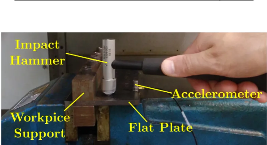
The SAE 1045 steel plate is one of the most used materials in engineering and, hence, is used as a workpiece material. (Davim and Maranhao, 2009). The material properties and the plate dimensions are presented in Table 1. An 80-mm-long plate is clamped, in a way that 55 mm are in balance. The dimensions and material properties are discussed later, and they are used as design variables on some model updating approaches. So, the values pre-sented in Table 1 will not be used in every situation covered in the present work. The fixturing system is composed of two square bars with five bolts, holding the plate in the vertical position, forming a cantilever plate. The bottom bar is directly fixed to the vise. To ensure the same clamping conditions and, therefore, repeatability, a torque wrench is used, applying 29 N.m to each bolt. The applied torque is high enough to prevent the workpiece from moving, but it is not too high, in order not to cause plastic deformation for the bolts. This clamping system is de-signed to hold the plate during a milling process. Figure 1 shows the experimental setup.
Table 1: Plate dimensions and material properties Young’s modulus (GPa) 210.0
Poisson’s ratio 0.3
Density (kg/m3) 7850.0
Length (mm) 80.0
Free length (mm) 55.0
Width (mm) 200.0
Thickness (mm) 6.2
Figure 1: Impact hammer modal testing setup
The experimental setup consists of the impact hammer, and a single axis accelerometer (oriented on the z-axis, normal to the plate’s plane), as shown in Figure 1. The signal is acquired with a SCXI-1531 signal conditioning module, from National Instruments, connected to a personal computer. A Brüel & Kjær 8206-003 impact hammer, with a sensitivity of 1.05 mV/N, is used. The accelerometer is a Brüel & Kjær 4397, whose sensitivity is 0.9931 mV/(m/s2). The signals measured in the time domain are converted to the frequency domain, using a Fourier transformation.
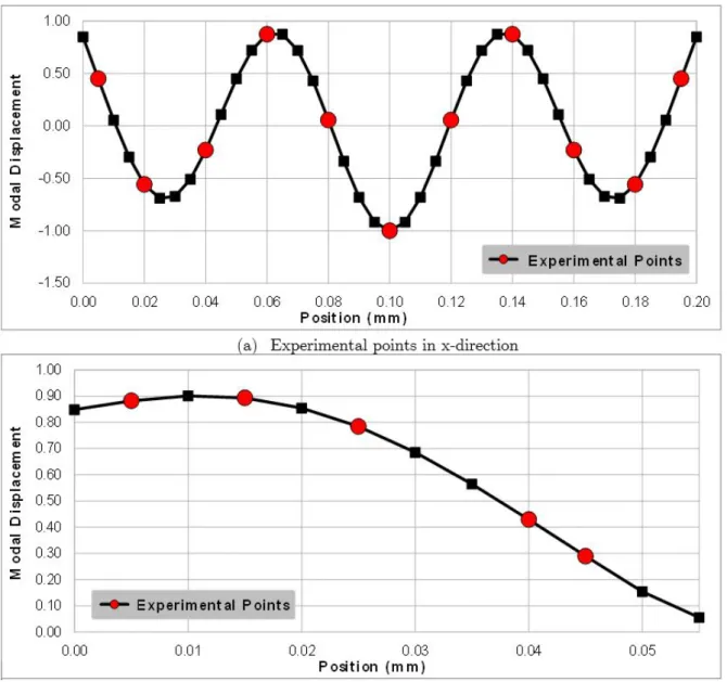
Figure 2: Determination of experimental points
To measure the natural frequencies, only one experimental point would be enough, if such point is not coinci-dent with any vibrational nodes. The procedure is basically hitting a determined point with the impact hammer and measuring the vibration on another point with the accelerometer. However, to acquire the eigenvectors’ experi-mental values, several points must be impacted or measured. The signal measured at the different points of the cantilever plate forms a symmetric matrix. A very useful physical meaning can be applied here: as that matrix is the same as its transpose, hitting a point and measuring another will generate the same results as hitting the second one and acquiring the data on the first one. This is called the reciprocity principle of the Frequency Response Func-tion (FRF). It can save a great amount of time, once fewer impact points are required (Ewins 1984).
length (x-direction) for the tenth modal shape is shown in Figure 2(a). The same procedure is performed in the y-direction at two different x-positions.
After that, based on the nodes of the numerical mesh, the position and number of experimental points which are capable of representing that modal shape are chosen. The points used to perform the modal experimental anal-ysis are plotted in red. A total of 55 points are then used and their coordinates are presented in Table 2.
Table 2: Experimental points position X-axis position (mm)
5 20 40 60 80 100 120 140 160 180 195
Y-axis position (mm)
45 45 46 47 48 49 50 51 52 53 54 55
40 34 35 36 37 38 39 40 41 42 43 44
25 23 24 25 26 27 28 29 30 31 32 33
15 12 13 14 15 16 17 18 19 20 21 22
5 1 2 3 4 5 6 7 8 9 10 11
The test procedure consists in attaching the accelerometer to point 1 and impacting all 55 points. An exponen-tial window is applied to the measured vibration signal. A frequency range from 1 Hz to 10 kHz, with a resolution of 1 Hz, is obtained from the FFT calculation. The first four natural frequencies are obtained from the frequency response functions, and the average of the 55 FRFs is calculated. The values of each mode measured on the 55 points did not present any variations greater than 1 Hz.
2.1 Experimental Eigenvectors Extraction
Once the experimental natural frequencies are known, the procedure to determine the modal shape can be performed. The eigenvectors provide important information about the dynamic behavior of the structure, and they can be combined to compose a matrix, in which each column is an eigenvector associated to an eigenvalue.
The eigenvectors are obtained for the first four natural frequencies. The experimental FRF for each of the 55 experimental points are represented in Table 3, where Ha,b is the response of the point a for the frequency b. The
method used to identify the modal parameter is the peak picking using the real and imaginary parts of the plate’s FRFs. This approach works well if the modes are not too closely spaced. The experimental eigenvectors are obtained from the imaginary part of the FRF at the corresponding natural frequencies for each of the 55 measured points.
Table 3: Experimental response for the 55 points on frequency domain Frequency (Hz)
1 2 3 4 fn1 fn2 fn3 10000
Experimental Point
1 H1,1 H1,2 H1,3 H1,4 H1,fn1 H1,fn2 H1,fn3 H1,10000
2 H2,1 H2,2 H2,3 H2,4 H2,fn1 H2,fn2 H2,fn3 H2,10000
3 H3,1 H3,2 H3,3 H3,4 H3,fn1 H3,fn2 H3,fn3 H3,10000
55 H55,1 H55,2 H55,3 H55,4 H55,fn1 H55,fn2 H55,fn3 H55,10000
3 FINITE ELEMENT ANALYSIS
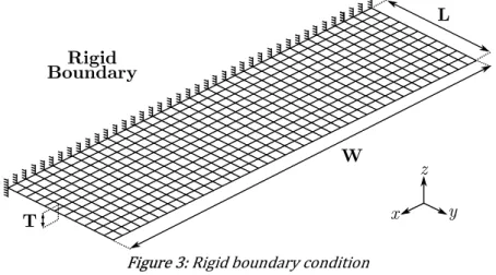
Figure 3: Rigid boundary condition
In the second model, translational springs in the z-direction (kUz) and rotational springs in the x-direction (kRx)
were added at the 41 nodes of the plate/clamping interface. That is demonstrated in Figure 4. The springs’ stiffness will be determined through the PSO method, which will be discussed later.
Figure 4: Boundary condition modelling using a rotational and a translational spring
For simplicity, the plate element of 4 nodes and the reduced integration (S4R) are adopted. It is important to notice that the selected element type is proper for thin plates. Therefore, the present work could be easily applied to thinner plates. However, if thicker plates were studied, there would be the need to use another element approach, such as Timoshenko thick plate theory, for example (Timoshenko and Woinowsky-Krieger, 1959).
To determine the mesh size, a refining analysis is performed. A number of 440 elements is found, 11 elements being along the y-axis and 40 elements distributed on the x-axis, as it can be seen in Figure 3. With such mesh configuration, square elements with an aspect ratio of 1 and side dimensions of 5 mm could be obtained. For the convergence analysis, the first four natural frequencies were monitored. This mesh configuration resulted in a num-ber of 492 nodes and 2952 degrees of freedom, and the mesh was applied to all models. One important part of the mesh definition is that every experimental point must coincide with a numerical node.
A modal analysis is performed in order to identify the natural frequencies and vibration modes, using the im-plicit module of ABAQUS 6.12. To protect the interest modes (the first four) from suffering variations caused by numerical error, the solution of the ten first natural frequencies and mode shapes (bigger than twice the interest frequency) was defined, ensuring a higher quality of the obtained response.
3.1 Modal Assurance Criterion
After performing the modal analysis, eigenvalues and eigenvectors are extracted from the experimental data. They are used to calculate the Modal Assurance Criterion (MAC), according to Equation (1),
{ } { }{ } { }
{ } { }{ } { }
bm am am bm
abm
bm bm am am
MAC
where the index a represents the experimental modes, which are compared to b, which are optimized numerical modes or rigid numerical modes. The index m is the mth mode. The Φ is the eigenvector associated with the mth
mode, and is the complex conjugate transpose (Hermitian operator) of a vector.
4 MODEL UPDATING
The model updating is an important tool in numerical simulations, used to create or modify a model, which can better represent a real situation. The focus of this paper is to simulate a real system, in order to properly represent the fixturing system of the cantilever plate in terms of its natural frequencies and modal shapes. Three different approaches were proposed and carried out, as shown in Table 4. It also shows the design variables used in each case, related to the clamping system, material and dimensional properties.
Table 4: Design variables for different model updating approaches 1st approach 2nd approach 3rd approach
Design Variables
kUz kUz kUz
kRx kRx kRx
Young’s Modulus Young’s Modulus Density Density
Free Length Width Thickness
4.1 Support Stiffness Updating Approach
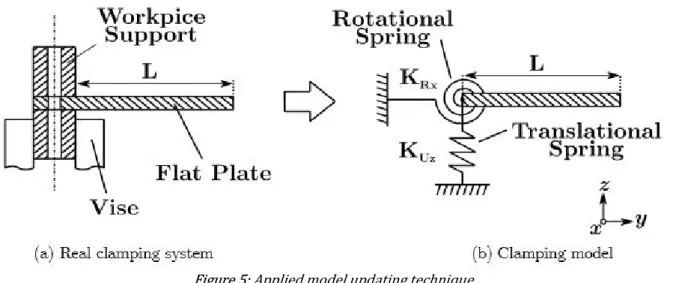
As discussed above, the fixture system, illustrated in Figure 5(a), does not provide a perfect encastre condition for the cantilever plate. Hence, the plate can move and rotate around the clamping region.
A model updating is applied using translational springs in the z-direction with stiffness kUz and rotational
springs in the x-direction with stiffness kRx. They are positioned on the nodes where the rigid clamping system is
supposedly located, in the plate/clamping interface, shown in Figure 5(b).
Figure 5: Applied model updating technique
1,1 1,2 1,3 1,4 1,5 1,6 1,24
2,1 2,2 2,3 2,4 2,5 2,6 2,24
3,1 3,2 3,3 3,4 3,5 3,6 3,24
4,1 4,2 4,3 4,4 4,5 4,6 4,24
5,1 5,2 5,3 5,4 5,5 5,6 5,24
6,1 6,2 6,3 6,4 6,5 6,6 6,24
2
Uz
Rx
k k k k k k k
k k k k k k k
k k k k k k k k
k k k k k k k k
K
k k k k k k k
k k k k k k k
k
4,1 k24,2 k24,3 k24,4 k24,5 k24,6 k24,24
(2)
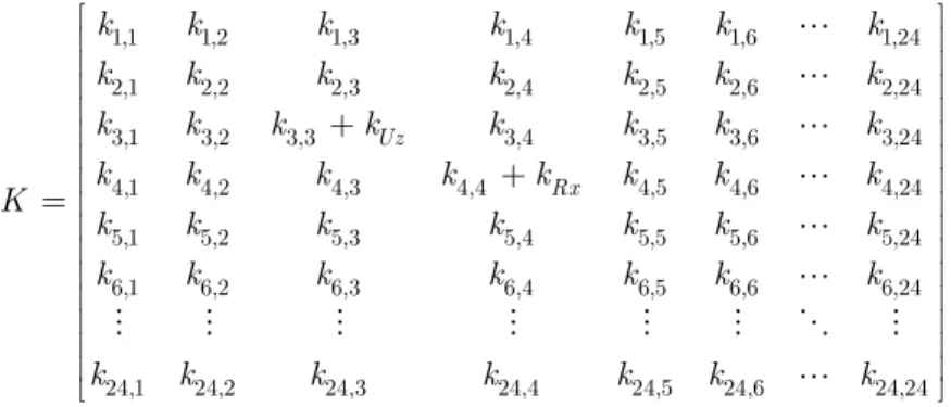
where K is the local 24x24 stiffness matrix, having 4 nodes with 6 degrees of freedom each. The three first degrees of freedom of a node are about the translation in x,y and z. The three last are related to the rotation of the same respective axis. This example is about the node 1 of the local coordinated system. This node is in the boundary zone, so the support’s stiffness is added to the diagonal of the stiffness matrix. The values are added to the main diagonal, once that is the position which relates a given degree of freedom for the force vector to the same degree of freedom for the displacement vector. The term about the translational stiffness in the z-direction is described as
3,3 3,3 Uz
k
k
k
(3)where k3,3 is the former term of the local stiffness matrix. The term related to the rotational stiffness in the
x-direction is
4,4 4,4 Rx
k
k
k
(4)The complete procedure adopted to the model updating approach is presented in Figure 6. The stiffness values for the springs kUz and kRx are generated according to the PSO algorithm (this optimization method will be discussed
later on section 5). After that, the finite element analysis is carried out using the software ABAQUS 6.12. The eigen-values and eigenvectors obtained through the simulation are compared to the ones obtained experimentally. This procedure is repeated until the stop condition is reached, resulting in the best configuration of stiffness found. The PSO algorithm is implemented in Python language. The simulation is performed using an Intel i5-2450M processor at the speed of 2.5 GHz.
Start Experimental Test Numerical Model Initial Springs Stiffness Running Simulation Error Estimation Adjust Springs Stiffness
Error ≤ Min End Impact Hammer Test FE Code Optimization Loop No Yes
4.2 Support Stiffness and Material Properties Updating Approach
This second approach is an extended version of the first one. It also focuses on finding a support stiffness which correctly represents the real fixturing system. In addition, it includes a contribution of the material properties. Both Young’s modulus and density of the workpiece are added as design variables as well, along with the previous used
kUz and kRx. This new approach is important, once the material properties are not the same every time, and they
may fluctuate within certain limits, as a function of several factors, especially the manufacturing process which generated the workpiece. This approach is more time consuming than the first one, once it has four design variables, instead of two. It also needs more iterations to find the final design variables. However, it might improve the model, with the ability to find closer natural frequencies and natural modes if compared to the experimental results. 4.3 Support Stiffness, Material Properties and Workpiece Dimensions Updating Approach
The third approach is the most comprehensive, and includes all the design variables presented on the second approach, adding three more. The new design variables are related to the workpiece’s dimensional tolerances, tak-ing variations on length, width and thickness into account. The workpiece’s dimensions are governed by the man-ufacturing process and their limits are set by technical standards. The simulation sequence is the same as the one presented in Figure 6, but seven design variables are updated instead of the spring’s stiffness only.
5 OPTIMIZATION
The particle swarm optimization method was originally developed by Eberchart and Kennedy (1995), consist-ing of an initial population, whose members locally interact with each other and are governed by global rules. The present papers uses the totally connected topology (gbest), which means a particle takes the whole population as its
topological neighbors.
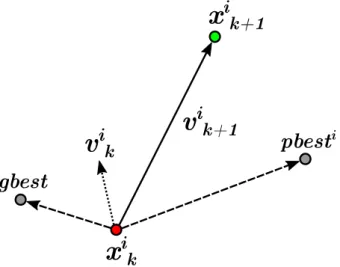
Initially, each particle has a random position and velocity. The particles interact with each other, informing the best position. With the data, the velocities and positions are adjusted for each particle. The velocity of a particle i
for the next increment (k+1) is given as
1 1 1( ) 2 2( ); 1,2,...,
i i i i i
k k best k best k
v wv C R p x C R g x i N (5)
where N is the total number of particles, R1 and R2 are random values from 0 to 1, pbest is the best position for that
particle, and gbest is the best global position. w, C1 and C2 are chosen parameters: the first one is an inertial
component of the particle, and the last ones are terms of “reliability” between the particles in the group (Perez & Behdinan, 2006). The position at the next iteration can be determined as
1 1; 1,2,...,
i i i
k k k
x x v i N (6)
here
x
ki is the position at the present iteration. Figure 7 shows the position and velocity of a particle in a step, andhow the best global position and the best particle position will influence the next particle position.
Ideally, a study about the best values of w, C1 and C2 must be performed, but there are standard suggested
values that work properly in most situations (Eberchart and Kennedy, 1995). Values between 0.8 and 1.4 are pro-posed for w, and 2 is proposed for C1 and C2. This work used a value of 0.8 for the inertial component and the
recommended value for C1 and C2. The next steps consist on defining the optimization problem, developing the
objective function and setting the parameters’ limits. 5.1 Updating Parameters’ Limits
The limits of the design variables are an important part of the optimization solution, and must be carefully defined. The present work uses up to 7 design variables, which can be divided into three groups: support stiffness, material properties and workpiece dimensions. Regarding the latter, the workpiece is a steel flat plate, and its thick-ness must comply with some tolerances, which are specified by a technical standard for a given manufacturing process (ASTM, 2017).
The two remaining dimensions, free length and width, have their limits as functions of their manufacturing processes as well. However, the cutting tolerance depends on the kind of process and is not defined by standard specifications. Instead, it is based on the manufacturer’s capacity. In this work, those tolerances were defined by measuring the workpiece. From such measurements, the standard deviation (based on a normal distribution) was calculated, and a 95,45% confidence level was chosen, resulting in
Pr(2 X 2 ) 0.9545 (7)
where μ is the mean, σ is the standard deviation, and X is a random variable which, from Equation (7), has a 95.45% chance of being inside the given interval. So, for the design’s width and length parameters, limits are set to be the mean values from the measurements, with a deviation of +2σ for the upper limits and -2σ for the lower limits.
The material properties elasticity modulus and density were chosen to be design variables from approaches 2 and 3 of the model updating modes. Those properties as commonly set as constant, but there is some variation, mainly due to the steel’s composition and its manufacturing process. The limits for the elasticity modulus were set based on experimental data from cold formed steel plates (Bernard et al., 1992). Variations of up to 5% from the standard Young’s Modulus were found (Mahendran, 1996), which can be considered small, but not negligible. The carbon steel’s density limits were determined by an analogue approach. Values as low as 7650 kg/m3 (Budynas &
Nisbett, 2011) and as high as 7950 kg/m3 (Taylor, 2005) were found in the literature, and were set as the lower
and upper limits for those design variables.
Finally, the two last design variables must be set: the translational springs in the z-direction (kUz) and the
rotational springs in the x-direction (kRx). Once they are unique for each support, they could not be set based on
previous works. To find their limits, several optimizations were performed, using a wide range of stiffness for both springs. After some optimization using different stiffness limits, the best value found for each simulation was com-puted, and limits were set. They include all best stiffness configurations found previously. Table 5 shows the limits used in the PSO algorithm.
Table 5: Design variables’ limits
Design Variables Lower Limit Upper Limit
kUz (N/m) 105 108
kRx (N.m/rad) 102 104
Young’s Modulus (GPa) 190 230 Density (kg/m3) 7650 7950
Free Length (mm) 55.25 55.81
Width (mm) 200.39 201.23
Thickness (mm) 5.97 6.43
5.2 Optimization Problem
exp
4 2
1 exp
1 ( )
2 num i i i i fn fn RMSE fn
(8)where fniexp is the natural frequency obtained experimentally for mode i, (reference value) and fninum is the natural
frequency for mode i obtained through numerical simulation.
The stiffness values of the translational kUz and the rotational kRx springs are adopted as design variables for
the first approach. They are inserted at the 41 nodes of the plate/clamping interface, modeled according to Figure 5(b). For this analysis, all translational springs are considered to have the same stiffness. The same is applied to the rotational springs. The minimum number of particles for each approach follows the criterion of the ten times the number of design variables. Four more experiments are performed, increasing the particle number by ten for each simulation. Thereby, five different numbers of particles are used in each approach, as shown in Table 6. For each number of particles, three cases are simulated, to ensure repeatability.
Table 6: Number of particles for each approach
Approach 1 Approach 2 Approach 3
Number of Particles
20 40 70
30 50 80
40 60 90
50 70 100
60 80 110
The optimization problem, representing the third approach, can be seen in Equation (9), exp 4 2 1 exp 1 ( , , , , , , ) ( ) 2 . . . num i i
Uz Rx i
i
Uz Uz Uz
Rx Rx Rx
fn fn Minimize f k k E l w t
fn
S T k k k
k k k E E E
L L L W W W
T T T
(9)The objective function can be seen on this equation, which must be minimized, as well as the limits to which the problem is subject (S.T.), consisting of the lower and upper limits of the design variables, 7 in this case. Those limits are specified in Table 5 for the three different cases. The present study used the standard PSO method (with-out any modifications).
Finally, to completely define the optimization problem, the stopping criteria must be defined. For the present work, three stopping criteria are set: the maximum number of iterations, the best position’s minimum step size and the best objective value’s minimum change. The first one is necessary to limit the simulation’s running time. If the intended minimum error is not met, the optimization loop will stop when it reaches the chosen maximum number of iterations. The second one basically monitors the best found positions and, if after some point, the best found position of the particle in a certain step is too close to the previous steps, meaning that the best particle is almost static, the stopping criterion is met. The last one is very similar to the previous, but instead of looking at the parti-cle’s position, it monitors the objective function. If the objective of the best value is sufficiently close to the last step, then it also means that, probably, the local or global minimum is reached, and the stopping criteria is met.
6 RESULTS
and to a simulation applying a rigid boundary condition. This last step is very important, once a rigid boundary condition is a pretty standard hypothesis, which is often applied without testing its validity.
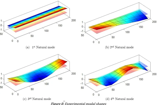
6.1 Experimental Modes and Frequencies
The experimental results for the modal analysis consist of the natural frequencies and their respective modal forms. Table 7 presents the natural frequencies obtained through the experiments. It is important to emphasize that the experimental analysis is able to detect only the first four natural frequencies, because the impact hammer test is able to excite only the workpiece’s frequencies below 4 kHz.
Table 7: Experimental natural frequencies 1st Natural Frequency (Hz) 1053
2nd Natural Frequency (Hz) 1379
3rd Natural Frequency (Hz) 2214
4th Natural Frequency (Hz) 3528
Each measured experimental natural frequency has a modal shape associated with it (eigenvectors), as shown in Table 3.
Figure 8: Experimental modal shapes
6.2 Model Updating Analysis and Convergence of the PSO Simulations
As described in Table 6, each of the three approaches is performed using 5 different numbers of particles. Three cases of each approach for a different number of particles were simulated and the best result was chosen. The minimum objective function error and the processing time are presented in Table 8.
Table 8: Minimum error for each approach and number of particles Approach
Simulation Error Approach 1 Approach 2 Approach 3
(%) Time (h) Error (%) Time (h) Error (%) Time (h) 1
2 3 4 5
2.94 2.9 0.79 3.6 0.18 4.3
2.90 4.3 0.59 4.8 0.14 7.7
2.95 5.3 0.51 6.0 0.15 10.7
2.95 6.1 0.49 7.5 0.13 11.2
2.95 6.9 0.52 8.8 0.14 11.7
The best result in terms of minimal RMSE is obtained for the third approach
(0.13), followed by the second (0.49) and the first (2.90). It is also important to observe that, for the first approach, increasing the number of particles does not reduce the error. For the second approach, the error de-creases from 0.79 to 0.49 when the number of particles inde-creases by 30. The same tendency is observed for the third approach, in which the error decreases from 0.18 to 0.13. However, the CPU processing time increases con-siderably with the number of particles.
The time increases at rate of 9.8%, 13.1% and 18.1% as the number of particles increases at a rate of 10 parti-cles, for the first, second and third approach respectively. Taking the influence of the design variables and the num-ber of particles on the error and time processing into account, it can be stated that the increase in design variables is more effective than the increase in the number of particles for all simulation results.
Figure 9 presents one convergence curve from the optimization process. The data are relative to one simula-tion of the third approach, using 100 particles. The iterasimula-tions and the Root Mean Square Errors are shown. It can be seen that, as expected, after each iteration, the error tends to be reduced and, after a certain number of iterations, it tends to stabilize, which means that the optimization loop is close to a local solution and a stop criterion might be reached soon. It can also be noticed that the variation of the particle tends to be smaller after every loop, mainly because the particles are closer to a local or global minimum. It is important to emphasize that the PSO does not ensure a global minimum.
6.3 Updated Model Frequencies and Parameters
The best results (minimum error on the objective function) found for each of the three model updating ap-proaches are presented in Table 9. It also shows the updated parameters, material and dimensional properties for each case. The results are also compared to a numerical simulation using a rigid boundary, as previously described. Analyzing the Root Mean Square Error (RMSE), the results obtained from the rigid boundary simulation can be seen to be far from the real situation, with an error of 49.33%.
Table 9: Updated parameters and natural frequencies
Rigid 1st Approach 2nd Approach 3rd Approach Experimental Values (Reference)
1st Natural Frequency
(Hz) 1812 1042 1054 1052 1053
2nd Natural Frequency
(Hz) 2115 1380 1378 1382 1379
3rd Natural Frequency
(Hz) 2966 2262 2204 2210 2214
4th Natural Frequency
(Hz) 4352 3714 3558 3530 3528
Kuz (MN/m) ∞ 2.15 5.54 98.05
Krx (N.m/rad) ∞ 1242.75 1102.66 1049.18
Young’s Modulus (GPa) 210.0 210.0 190.0 193.7 Density (kg/m3) 7850.00 7850.00 7950.00 7921.76
Free Length (m) 0.0550 0.0550 0.0550 0.0558 Width (m) 0.2000 0.2000 0.2000 0.2012 Thickness (m) 0.00620 0.00620 0.00620 0.00609
RMSE (%) 49.33 2.90 0.49 0.13
The smallest error found is 0.13% for the third approach. However, all three model updating approaches are able to accurately model the experimental natural frequencies. It is important to notice that the optimization rou-tine for the third approach found greater values for translational spring stiffness (almost 50 times greater than the 1st approach). However, a smaller thickness is obtained, which means that the third approach has a more rigid fixturing system and a more flexible plate.
Figure 10 shows the natural frequencies found for each approach and compares them to the experimental results, which are the reference values. A 10% tolerance is set (dashed lines).
It can be noticed that, for the rigid boundary approach, the natural frequencies are off limits, while for the other approaches the frequencies are very close to the experimental results.
6.4 Updated Model Modal Shapes
Even though the optimization routine only took the comparison between the experimental natural frequencies and the numerical ones into account, the modal shapes of the models are an important part of the problem. A good model must be able to represent both natural frequencies and modal shapes properly. Figure 11 shows the Modal Assurance Criterion, which compares the experimental modal form (the reference value) to the numerical ones.
Figure 11: MAC number of numerical modes compared to experimental ones
It can be seem that, if a rigid boundary is applied to model the real problem, the modal shapes will be poorly represented, far from the real condition. The best results on MAC are found using the first model updating approach, which uses two springs as design parameters, as shown in Table 4. This is mainly due to the low translational stiff-ness spring, which better representes the real fixture system’s flexibility. The third approach represents the modal form better than the simulation using a rigid boundary, but worse than the second approach.
followed by the second and third approaches. The rigid boundary, as expected, is the worst model to this situation as well. It can be noticed that this model results in much smaller displacements when compared to the real situation.
Figure 12: Comparison of modal displacements close to the clamping system for the 4th mode
7 CONCLUSIONS
The main goal of this work is to properly model a cantilever plate clamped at a non-ideal fixture system in order to correctly predict its natural frequencies and modal shapes. Simulations using FEM are performed in order to calculate the dynamic characteristics of the workpiece. Therefore, the measured and simulated natural frequen-cies and mode shapes differ mainly because of the encastre condition, considered ideally rigid. A model updating technique is applied based on a PSO algorithm, and three different approaches are investigated. In the first one, the encastre condition is modeled with a translational and a rotational spring linked to the nodes of the finite elements at the clamping region. Material properties variation is added to the first approach as a design variable, constituting the second approach. Finally, the third approach adds workpiece’s geometrical variation. The results show that the average natural frequency error is reduced from about 49% for the rigid model to less than 3% for the first model updating approach, and 1% for the second and third approaches. The design variables show to be more effective than increasing the number of particles to minimize the error and processing time. It is observed that, with the update of the natural frequencies, the modal shapes are improved as well. This is observed through the MAC anal-ysis. Before the model update, the average MAC is 0.93. After the optimization, it is increased to 0.98. The third approach found the best solutions to the natural frequencies. However, the first approach represented the best modal shapes, mainly due to the low stiffness spring configuration found by the PSO algorithm. The second one presents an intermediate solution. The same tendency is observed in the normalized modal displacement at the nodes from the FE model close to the encastre, where the first approach gives results that are close to the experi-mental ones. Although increasing the number of updated parameters regarding material’s properties and work-piece’s geometry reduces the error in the natural frequencies by 2%, the processing time increases considerably, and the MAC and modal displacements are worse. Thereby, a model update considering only the stiffness at the encastre region, through the modeling by translational and rotational springs (first approach), shows to be the best solution to model the cantilever plate in this case.
References
Ahmadian, H., Mottershead, J., Friswell, M. (1998). Regularization methods for finite element model updating 12: 47-74.
ASTM. (2017). Standard Specification for Steel, Sheet, Carbon, Structural, and High-Strength, Low-Alloy, Hot-Rolled and Cold-Rolled, General Requirements for. West Conshohocken: ASTM.
Baruch, M. and Bar Itzhack, I. Y. (1978). Optimal Weighted Orthogonalization of Measured Modes. AIAA journal 16: 346-351.
Berman, A. and Nagy, E. (1983). Improvement of a large analytical model using test data. AIAA journal 21: 1168-1173.
Bernard, E. S., Bridge, R. Q., Hancock, G. J. (1992). Tests of Profiled Steel Decks with V-stiffeners. International Spe-cialty Conference on Cold-Formed Steel Structures.
Boyle, I., Rong, Y., Brown, D. C. (2011). A review and analysis of current computer-aided fixture design approaches. Robotics and Computer-Integrated Manufacturing 27: 1-12.
Budynas, R. G. and Nisbett, J. K. (2011). Shigley's Mechanical Engineering Design. New York: Mc Graw Hill.
Bussetta, P., Shiki, S. B., Silva, S. d. (2017). Updating of a Nonlinear Finite Element Model. Latin American Journal of Solids and Structures 14: 1183-1199.
Davim, J. and Maranhao, C. (2009). A study of plastic strain and plastic strain rate in machining of steel AISI 1045 using FEM analysis. Materials and Design 30: 160-165.
Eberchart, R. and Kennedy, J. (1995). Particle swarm optimization. IEEE International Conference on Neural Net-works.
Ewins, D. J. (1984). Modal testing: theory and practice (Vol. 15). Letchworth: Research studies press.
Friswell, M. and Mottershead, J. E. (2013). Finite element model updating in structural dynamics. Netherlands: Springer.
Galewski, M. A. (2016). Spectrum-based modal parameters identification with particle swarm optimization. Mecha-tronics, 37: 21-32.
Jaishi, B. and Ren, W.-X. (2007). Finite element model updating based on eigenvalue and strain energy residuals using multiobjective optimization technique. Mechanical Systems and Signal Processing 21: 2295-2317.
Kabe, A.M. (1984). Constrained Stiffness Matrix Adjustment Using Mode Data. Air Force System Command, Space DIvision. Los Angeles: DTIC Document.
Mahendran, M. (1996). The Modulus of Elasticity of Steel - Is It 200 GPa? International Specialty Conference on Cold-Formed Steel Structures.
Marwala, T. (2007). Dynamic Model Updating Using Particle Swarm Optimization Method. arXiv preprint arXiv:0705.1760.
Moradi, S., Fatahi, L., & Razi, P. (2010). Finite element model updating using bees algorithm. Structural and Multi-disciplinary Optimization, 42(2), 283-291.
Mottershead, J., Friswell, M., Ng, G., Brandon, J. (1996). Geometric parameters for finite element model updating of joints and constraints. Mechanical Systems and Signal Processing 10: 171-182.
Plevris, V., and Papadrakakis, M. (2011). A hybrid particle swarm—gradient algorithm for global structural optimi-zation. Computer‐Aided Civil and Infrastructure Engineering, 26(1), 48-68.
Sehgal, S., & Kumar, H. (2016). Structural dynamic model updating techniques: A state of the art review. Archives of Computational Methods in Engineering, 23(3), 515-533.
Seyedpoor, S. M. (2012). A two stage method for structural damage detection using a modal strain energy based index and particle swarm optimization. International Journal of Non-Linear Mechanics, 47(1), 1-8.
Taylor, J. R. (2005). Classical Mechanics. Colorado: University of Colorado.
Timoshenko, S. P., & Woinowsky-Krieger, S. (1959). Theory of plates and shells. New York: McGraw-hill.