Business Cycle Synchronization and Insurance Mechanisms in the EU

Carlos Pestana Barros & Nicolas Peypoch

A Comparative Analysis of Productivity Change in Italian and Portuguese Airports

WP 006/2007/DE _________________________________________________________

António Afonso and Davide Furceri

Business Cycle Synchronization and Insurance Mechanisms in the EU

WP 026/2007/DE/UECE

Departament of Economics

WORKING PAPERS

ISSN Nº0874-4548

Business Cycle Synchronization and

Insurance Mechanisms in the EU

António Afonso,

Davide Furceri

2007

Abstract

In this paper we provide a positive exercise on past business-cycle correlations and risk sharing in the European Union, and on the ability of insurance mechanisms and fiscal policies to smooth income fluctuations. The results suggest in particular that while some of the new Member States have well synchronized business cycles, for some of the other countries, business cycles are not yet well synchronized with the euro area’s business cycle, and risk-sharing mechanisms may not provide enough insurance against shocks.

JEL: E32; E42; F41; F42

Keywords: EU, Optimum Currency Areas, Business Cycle Synchronization, Insurance Mechanisms

*

We are grateful to Jürgen von Hagen, José Marín, Vito Tanzi, participants at seminars at the ECB, at the University of Barcelona, at the 11th International Conference on Macroeconomic Analysis and International Finance, an anonymous referee for helpful comments, and Renate Dreiskena for research assistance. The opinions expressed herein are those of the authors and do not necessarily reflect those of the ECB or the Eurosystem.

#

European Central Bank, Directorate General Economics, Kaiserstraße 29, D-60311 Frankfurt am Main, Germany, email: antonio.afonso@ecb.int.

$

ISEG/TULisbon – Technical University of Lisbon, Department of Economics; UECE – Research Unit on Complexity and Economics, R. Miguel Lupi 20, 1249-078 Lisbon, Portugal, email: aafonso@iseg.utl.pt. UECE is supported by FCT (Fundação para a Ciência e a Tecnologia, Portugal), financed by ERDF and Portuguese funds.

+ _{University of Palermo, Department of Economics, Italy.}

%

Contents

Non-technical summary ... 3

1. Introduction... 5

2. Empirical Methodology ... 7

2.1. Business Cycle Synchronization ... 7

2.2. Risk Sharing and Insurance Mechanisms... 9

2.3. Fiscal Policies ... 11

3. Empirical Analysis... 12

3.1. Data... 12

3.2. Business Cycle Synchronization ... 13

3.3. Insurance Mechanisms ... 15

3.4. Income Smoothing and Fiscal Policies... 18

4. Conclusion ... 19

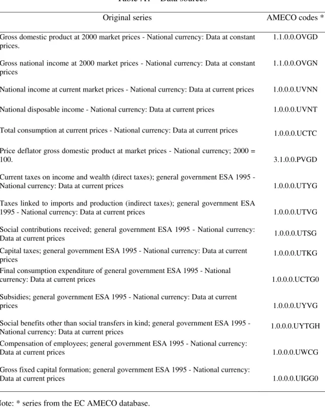
Annex – Data Sources... 21

References... 23

Tables and Figures ... 26

Non-technical summary

On 1 May 2004 the European Union (EU) welcomed ten new members: the Czech

Republic, Estonia, Cyprus, Latvia, Lithuania, Hungary, Malta, Poland, Slovenia and

Slovakia. In addition, two other countries, Bulgaria and Romania, joined the EU on

January 2007, and other three countries are at various stages of candidacy for membership

in the EU: Croatia, Turkey and the Former Yugoslav Republic of Macedonia.

The theory of Optimum Currency Areas (OCA) has long stressed the importance of

the synchronization in cyclical economic activity and insurance mechanisms for members

of a monetary union. At the same time effective insurance mechanisms could offset

asymmetric shocks eventually affecting the new and the old EU members.

This study discusses only one of many aspects which are relevant for an assessment

of the advantages of joining the euro area and of the costs and risks of a premature

introduction of the euro. It does not discuss in detail many other important determinants of

a successful participation in the euro area, such as sustainable price stability, sound fiscal

policies, efficient structural policies and a high degree of price and wage flexibility, which

are outside the scope of this paper. Indeed, the purpose of the paper is not to draw overall

conclusions on the benefits and costs of joining the euro area.

Using annual data for 28 countries (the 12 EMU countries up to the end of 2006,

one country that adopted the euro in the beginning of 2007, the 3 existing EU countries

which have not adopted the euro, the 9 new EU members also outside the euro, and 3

prospective members, Bulgaria, Romania and Turkey) from 1980 to 2005, we evaluate

how important these determinants are, within current EMU and in the EU. We use data on

real GDP, gross national product, national income, disposable national income, private

identify channels of risk-sharing that exist in the EU25 and in EMU. We use fiscal data to

evaluate the ability of fiscal policies to smooth shocks.

With regard to the first determinant, the results of the paper show, for the period

1980-2005, that there is a variety of situations as regards business cycle synchronization.

With regard to the second determinant, our results show that, overall and as things

stand now, in an enlarged EMU the ability to smooth country-specific shocks does not

increase. In fact, while (for the more recent period 1998-2005) the amount of shock to

GDP unsmoothed in the current EMU is 63 percent, in an enlarged EMU at 25 members it

would be 69 percent. However, this result is not driven by the effectiveness of fiscal

variables, since they seem to work better for stabilisation purposes in an enlarged EMU

than in the current EMU.

However, it should be noticed in this regard that this analysis can provide useful

indications only in the short to medium term. Moreover, the amount of cross-sectional

smoothing would increase as EMU and other EU countries could become more

homogenous in terms of risk-sharing channels. Thus, both business cycle synchronization

and international risk-sharing are likely to increase as the integration of the new member

countries' economies within the European Union progresses, and will be further enhanced

1. Introduction

On 1 May 2004 the European Union (EU) welcomed ten new members: the Czech

Republic, Estonia, Cyprus, Latvia, Lithuania, Hungary, Malta, Poland, Slovenia and

Slovakia. In addition, two other countries, Bulgaria and Romania, joined the EU on

January 2007, and other three countries are at various stages of candidacy for membership

in the EU: Croatia, Turkey and the Former Yugoslav Republic of Macedonia.

As underlined during the accession negotiations, once these countries have

achieved economic and budgetary results in line with the Maastricht Treaty, they are

expected to join the single currency (Slovenia joined on January 2007). None of the

countries requested a dispensation and no ‘opt-out’ options were granted. This means that

the new (and, eventually, the prospective) EU countries should be considered candidates

for the euro once they join the EU.

The theory of Optimum Currency Areas (OCA) has long stressed the importance of

the synchronization in cyclical economic activity and insurance mechanisms for members

of a monetary union.1 In particular, the higher the correlation of business cycles, the lower

the stabilization cost of giving up an independent monetary policy. Intuitively, if a

member economy’s business cycle is very highly correlated with the union-wide cyclical

output, then monetary policy conducted by the common central bank will be a very close

substitute for the country’s own independent monetary policy. If, on the other hand, the

economy’s business cycle is weakly correlated (or, worse, negatively correlated) with the

union’s cyclical output, then the common monetary policy will be a poor substitute for that

economy’s own independent monetary policy, and may end up actually being

1

destabilizing. At the same time effective insurance mechanisms could offset asymmetric

shocks eventually affecting the new and the old EU members.

This study is a positive exercise on past business cycle correlations and risk

sharing and discusses only one of many aspects which are relevant for an assessment of the

advantages of joining the euro area and of the costs and risks of a premature introduction

of the euro. It does not discuss in detail many other important determinants of a successful

participation in the euro area, such as sustainable price stability, sound fiscal policies,

efficient structural policies and a high degree of price and wage flexibility, which are

outside the scope of this paper. Indeed, the purpose of the paper is not to draw overall

conclusions on the benefits and costs of joining the euro area.

Therefore, the aim of this paper is to evaluate how important these two OCA

criteria are in the euro area and in the EU. We use annual data on real GDP, gross national

product, national income, disposable national income, private consumption and public

consumption to evaluate business cycle synchronization and to identify channels of

risk-sharing that exist in the EU25 and in EMU. We use fiscal data to evaluate the ability of

fiscal policies to smooth shocks. The results of the paper suggest a variety of situations as

regards business cycles synchronisation and risk-sharing mechanisms.

The remainder of the paper is organized as follows. In Section Two we present the

empirical methodology used to evaluate costs from entering in the EMU. Section Three

reports the results obtained, and finally, Section Four summarises the paper’s main

2. Empirical Methodology

2.1. Business Cycle Synchronization

Business cycle measures are obtained by detrending the series of real GDP. Four

different methods are used to detrend the output series of each country i and estimate its

cyclical component. Lettingy_i,t =ln

( )

rate of the real GDP):

ci,t = yi,t − yi,t−1. (10)

The second and the third method use the Hodrick-Prescott (HP) filter, proposed by

Hodrick and Prescott (1980). The filter decomposes the series into a cyclical

( )

trend

( )

parameterλ >0 the following quantity:

(

)

(

)

∑

∑

i g g g

y 1 1 2 2 1 , 1 , 2 ,

, λ . (1)

The methods differ because the second one consists of using the value

recommended by Hodrick and Prescott for annual data for the smoothness parameter (λ)

equal to 100, while the third method considers the smoothness parameter (λ) to be equal

to 6.25. In this way, as pointed out by Ravn and Uhlig (2002), the Hodrick-Prescott filter

produces cyclical components comparable to those obtained by the Band-Pass filter.

The fourth method makes use of the Band-Pass (BP) filter proposed by Baxter and

King (1999), and evaluated by Stock and Watson (1999) and Christiano and Fitzgerald

(2003) (who also compares its properties to those of the HP filter). The Low-Pass (LP)

filter α(L), which forms the basis for the band pass filter, selects a finite number of

∫

= π

π δ ω dω

Q ( )2 , (2)

where =

∑

K h

h hL

L α

α( ) and =

∑

K h

h i h

K e

ω

α ω

α ( ) .

The LP filter uses α_K(ω) to approximate the infinite MA filter β(ω). Defining

) ( ) ( )

(ω β ω α ω

δ ≡ − , and then minimizing Q, we minimize the discrepancy between the

ideal LP filterβ(ω) and its finite representation α_K(ω) at frequency ω. The main

objective of the BP filter as implemented by Baxter and King (1999) is to remove both the

high frequency and low frequency component of a series, leaving the business-cycle

frequencies. This is obtained by subtracting the weights of two low pass filters. We define

L

ω and ω_H, the lower and upper frequencies of two low pass filters, as respectively eight

and two for annual data. We therefore remove all fluctuations shorter than two or longer

than eight years. The frequency representation of the band pass weights becomes

) ( )

( _{H K L}

K ω α ω

α − , and forms the basis of the Baxter-King filter, which provides an

alternative estimate of the trend and the cyclical component.

The three filters yield substantially similar results, with only minor differences (for

example, differencing generally produces the most volatile series, while the BP the

smoothest). This robustness will be formally assessed by the estimations of the empirical

section.

Finally, we measure business cycle synchronization for each country as the

correlation between the country’s cyclical component and EMU’s cyclical component, ci:

2.2. Risk Sharing and Insurance Mechanisms

In order to quantify the grade of risk-sharing through different channels, we follow

Asdrubali et al. (1996) and decompose GDP into different income national aggregates all

closely tied to GDP: Gross National Product (GNP), Net National Income (NI), Disposable

National Income (DNI), and Total (private and public) Consumption (C+G):

GDP-GNP = international income transfers (factor income flows), (4)

GNP-NI = capital depreciation,

NI-DNI = netinternational tax and transfers,

DNI-(C+G) = total saving.

If a shock hits the economy of one country, modifying the value of the GDP, the

economic system will smooth the shock if some counter-cyclical factor can perform this

task.

Let us consider the following chain equation between GDP and total consumption:

(

) (

)

i i i

i i

i i i

i C G

G C

DNI DNI

NI NI GNP GNP GDP

GDP ⋅ +

+ ⋅ ⋅ ⋅

= . (5)

If only GDP varies after the shock, while the other aggregates are unchanged, then

full stabilisation has been obtained. If GDP varies and GNP remains unchanged, on the

other hand, then stabilisation is achieved in the first stage by the international net transfers

of income factors. Conversely, if GNP varies and NI remains constant, then cyclical

smoothing is provided by the capital depreciation. Finally, if the total consumption also

In principle, all these factors (except capital depreciation) have a counter-cyclical

smoothing effect. The first aggregate expresses the international transfers of the income

that is earned by foreign entities in each country. The second aggregate is the capital

depreciation, usually calculated as a constant part of the total amount of capital. Thus,

since the capital-to-output ratio is typically counter-cyclical, depreciation will constitute a

large fraction of output in recessions and a smaller fraction in boom periods, resulting in a

higher cross-sectional variance of NI with respect to GNP. The third aggregate is based on

the mutual insurance between the countries. Finally, the fourth aggregate represents

consumption smoothing.

In particular, from equation (5) it is possible to derive2 the following system of

independent equations (with time fixed-effects):

m t i t i m m t t i t

i GNP GDP

GDP_, log _, log _{, ,}

log −∆ =α +β ∆ +ε

∆ d t i t i d d t t i t

i NI GDP

GNP_, log _, log _{, ,}

log −∆ =α +β ∆ +ε

∆ g t i t i g g t t i t

i DNI GDP

NI_, log _, log _{, ,}

log −∆ =α +β ∆ +ε

∆ (6)

(

)

t i t i s s t t i t

i C G GDP

DNI _, log _, log _{, ,}

log −∆ + =α +β ∆ +ε

∆

∆log

(

)

where the index i

(

)

(

)

period and α_t stands for time fixed-effects.

The β coefficients measure the incremental percentage amount of smoothing

achieved at each level of the GDP decomposition, and

∑

percentage of shock that remains unsmoothed; βm is the percentage of shock smoothed by

2

factor income flows; βd represents capital depreciation smoothing (or dis-smoothing); βg is

the amount of shock smoothed by international transfers; βs measures consumption

smoothing. Thus, if βu=0, then there is full risk-sharing. Moreover, each coefficient has no

constraint, so it can be either larger than 1 or negative (dis-smoothing).

The time fixed-effect captures year-specific impacts on growth rates. To take into

account autocorrelation in the residuals, we assume that the error terms in each equation

and in each country follow an AR (1) process. We also allow for country-specific variance

of the error terms, since GDP is typically more variable for small countries. In practice, we

estimate the system (6) using a two-step General Least Squares (GLS) procedure.

2.3. Fiscal Policies

Considering equation (15) and decomposing

₍

₎

i i

G C

DNI

+ into

(

)

(

)

i i i

i i

DNI DNI DNI f

C G DNI f C G

+

= ⋅

+ + + , (7)

where f is the fiscal variable that we examine, we can differentiate between the effect of

consumption smoothing through fiscal policy and the effect of consumption smoothing

through private saving.

Using the same strategy proposed by Asdrubali et al. (1996) that we applied for

equation (16), we measure the fraction of the shock smoothed via government

consumption, transfer and taxes at EMU (or EU) level by estimating the coefficient in the

following panel regression (with time fixed-effects):

(

)

t i t i f

f t t i t

i DNI f GDP

DNI _, log _, log _{, ,}

log −∆ + =α +β ∆ +ε

In particular, the sign in parenthesis would be positive if we consider government

consumption, transfers or other government expenditures. In contrast, if we consider taxes

the sign will be negative.

Again, we assume that the error terms in each equation and in each country follow

an AR (1) process and we allow for country-specific variances. In practice, we estimate (8)

using a two-step GLS.

3. Empirical Analysis

3.1. Data

We use data from the Annual Macro-economic Database (AMECO).3 The dataset

covers 28 countries (the 12 current EMU countries, the 3 existing EU countries which have

not adopted the euro, the 10 new EU members, and 3 prospective members, Bulgaria,

Romania and Turkey) from 1980 to 2005.

The income variable we use to determine business cycle synchronization is real

GDP in 2000 constant prices. Data for real GNP, NI, DNI, C and G are also used to

estimate the effectiveness of insurance mechanisms4.

Fiscal variables (namely, Direct Taxes, Indirect Taxes, Social Contributions,

Capital Taxes, Subsidies, Social Benefits, Social Transfers, Government consumption,

Compensation of Employees, Gross Fixed Capital Formation) are used to estimate the

effect of fiscal policy on smoothing shocks.5

3

See Annex for a description of data sources and availability.

4

We use aggregate date in levels for these variables and not in per capita terms in order to make the analysis more comparable to the previous section. In fact, in terms of business cycle synchronization we also use as a measure of business cycle the growth rate of aggregate GDP. Moreover, since our dependent variables in equation (6) are differences of growth rates the use of aggregate level data instead of per capita data produce very similar results.

5

3.2. Business Cycle Synchronization

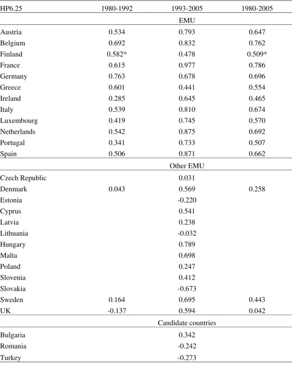
In Table 1, we calculate the correlation coefficient of each country’s cyclical

component of real GDP with that of EMU,6 as a whole, using the HP filter with

smoothness parameter equal to 6.25.7 The table considers three different periods of

analysis. The first is from 1980 to 1992 and considers the EU15 countries. The second is

from 1993 to 2005 and applies to all 28 countries. The third is the overall period from

1980 to 2005.

[Table 1 here]

In relation to the overall period, we can see that for most EMU countries business

cycle is relatively well synchronized, and France is the country with the highest

synchronization (0.786).

Looking at the period 1993-2005 it is clear that France shows an almost perfect

correlation with the EMU economy as a whole. However, comparing the 12 euro area

countries with the 3 (old) non-euro economies, it is difficult to establish a systematic

relationship. In fact, Denmark, Sweden and the UK appear to be more synchronized with

the EMU-wide cycle than some euro area members, such as Greece and Finland.

The new EU countries show a generally higher synchronization with the EMU than

the candidate countries. In particular, there are some new EU countries (such as Cyprus,

Hungary and Malta) already well synchronized with the EMU, and with correlations

comparable to, or even higher than, those of some of the old members.8 On the other hand,

6

It is possible to argue that the results of this analysis could be mainly driven by the home bias, due to the fact that EMU countries unlike other countries in the sample are already part of the EMU. However, since the size of the new and candidate members is very small compared to the EMU members the home bias is very negligible.

7

Even though the estimated correlations vary according to the detrending method used, the implied rankings are very similar, regarding the overall period, the highest Spearman’s rank correlation coefficients is 0.936 (BP, HP6.25) and the lowest is 0.776 (Diff, HP100). For a detailed comparison see Appendix 1.

8

several new EU countries (such as Estonia, Lithuania and Slovakia) exhibit negative

correlations, as do two of the three prospective EU members (Romania and Turkey).

Focusing on the 1980-2005 period is again fully feasible only for the old EU

members, but this can be used to indicate how the correlations have changed for these

countries, and how they could change for the prospective Member States. The most

striking fact to emerge from this exercise is that the degree of synchronization with EMU

has remarkably increased for all countries (with the exception of Germany, where it

remained broadly similar).9 This can largely be attributed to the achievement of a more

integrated market since 1992, and to an increase in trade as pointed out by Furceri and

Karras (2006). But, perhaps more unexpectedly, the results show that the increased

synchronization has been at least as large in the non-euro area as in the euro area

economies. The UK’s business cycle synchronization has seen the most dramatic change,

rising from -0.137 to 0.594. The policy implication of this is obvious. Seen from the point

of view of the whole period, the UK, Denmark, and Sweden are poor candidates for the

euro, as stabilisation costs would be very high. However, from the perspective of the

shorter period 1993-2005, the UK and Denmark appear to be highly correlated with the

EMU, changing the cost calculus.

In Figures 1 and 2 we compute the rolling-windows estimation for business cycle

synchronization. Looking at the figures, we can see that while a sort of convergence

Hungarian and Polish business cycles are similar to the euro area cycle. Darvas and Szapáry (2005) investigated the behavior of several expenditure and sectoral components of GDP. They found that GDP, industrial production, and exports in Hungary, Poland, and Slovenia have achieved a reasonably high degree of correlation with the euro area.

9

emerges among the EU15 members (even if not smoothly), there is no convergence among

the new EU and candidate countries.10

[Figure 1 here]

[Figure 2 here]

Additionally, it is worthwhile mentioning that this analysis can only provide a

useful indication in terms of stabilisation costs in the short to medium term. In fact, as

Frankel and Rose (1998) show, business cycle synchronization is likely to increase for the

EU countries once they join EMU. Moreover, EU membership could increase intra-EMU

trade allowing business cycle to become more synchronized11. Thus, the ex ante cost to

join the EMU is likely to be larger than the ex post cost.

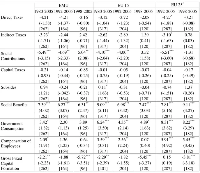
3.3. Insurance Mechanisms

In Table 2, we present the estimated percentages of shocks to GDP smoothed

through each channel pointed out in the GDP decomposition in (14), among EMU and EU

countries12. In particular, we consider two different sets of EU countries: the old EU

countries (EU15) and the overall EU countries including also the new ones (EU25). We

consider again three different periods of analysis. The first is from 1980 to 2005, the

second is from 1992 to 2005, and the third is from 1998-2005. In this way, we can see how

the ability of these channels to smooth income fluctuations evolves over time.

10

It is important to stresss that many of the new EU member countries have been in a transition period during which many institutional changes have been taking place. Thus, it could lead to somewhat misleading results to compare these economies with more mature economies. Neverthless, since we focus just on short run movements of GDP and not on stuctural changes, our analysis can still offer important indication about the process of convergence in business cycle syncronization.

11

See, for example, Artis and Zhang (1997), Frankel and Rose (1998), Rose and Engel (2002), Fidrmuc (2001, 2004), Fidrmuc and Korhonen (2006), Maurel (2002), and Rose and Stanley (2005).

12

[Table 2 here]

Analyzing the overall period from 1980 to 2005, it is immediately apparent that a

large amount of the shocks to GDP are not smoothed both for the EMU (57 percent) and

for the EU15 (61 percent) countries.13 In particular, factor income flows and international

transfers have a very negligible effect on income smoothing since they absorb respectively

1 percent (-0.25 percent) and 2.14 percent (2.39 percent) of shocks to GDP among EMU

(EU15) countries.

Capital depreciation provides dis-smoothing (around 6 percent for EMU and 8

percent for EU15 countries) since it generally constitutes a large fraction of output in

recessions and a smaller fraction in boom.

The only operative smoothing mechanism is consumption smoothing through

saving.14 For the EMU countries, and still for the overall period, saving is able to reduce

39 percent of shocks to GDP, and it reduces 37 percent of the shock among EU15

countries. Overall, looking at the entire period, it seems that the current EMU is able to

provide more income smoothing than an enlarged EMU at 15 members.

Looking at the period 1992-2005 we can see that income smoothing is increased

among both EMU and the EU15 countries.15 In particular, saving is able to smooth a larger

amount of shock to GDP (around 50 percent for both EMU and EU15 countries), and

factor income flows provide a small and statistically significant contribution to the amount

of shock smoothed (around 7 percent for EMU countries and 5 percent for EU15

countries). Comparing the results among the different sample of countries, we can see that

13

Using the same methodology for the US, Asdrubali et al. (1996) find that the amount of interstate risk-sharing not smoothed is only 25 percent of shocks to gross domestic product.

14

These results are consistent with those found by Sorensen and Yosha (1998).

15

overall insurance mechanisms work in the same way among EMU and EU15 countries. In

contrast, they provide less income smoothing among the EU25. In fact, comparing the

EMU and the EU25, we can see that while for the euro area countries 50 percent of the

shock is not smoothed, for the EU25 countries 64 percent of income fluctuations are not

absorbed. This implies that insurance mechanisms work better in the current EMU than in

an enlarged EU at 25 members.

The same conclusions emerge if we repeat the same comparison for the period

1998-2005. Moreover, it is also true that for all subsets of countries, the amount of

consumption-smoothing through saving is remarkably reduced, thus implying a larger

amount of unsmoothed shock.

It is important to notice that the period 1998-2005 provides more useful

indications in terms of income smoothing comparison between the actual EMU and an

enlarged EMU than the other periods. In fact, for this period our panel data set is fully

balanced, which means that the amount of risk-sharing in each country enters with the

same weight in the computation of the total amount of shock to GDP that is not smoothed.

Thus, it would seem that, overall, in an enlarged EMU the ability to smooth

country-specific shocks is softened.

Again, it is also worthwhile mentioning that this analysis can only offer some

useful indications in terms of stabilisation costs only in the short to medium term. As EMU

and other EU countries become more homogenous in terms of the channels investigated in

our analysis, the amount of cross-sectional smoothing may well increase. In fact, the

potential for risk sharing is likely to increase as the integration of the new member

countries' economies within the European Union progresses, and will be further enhanced

sharing across euro area countries since the 1990s, which however does not reach the level

observed for US states (see Giannone and Reichlin, 2006).

3.4. Income Smoothing and Fiscal Policies

In Table 3 we present the estimated percentages of shocks to GDP smoothed

through fiscal policies among EMU, EU15 and EU25 countries.16 This table also considers

the three different periods of analysis (1980-2005, 1992-2005, and 1998-2005). In this

way, we can see how the ability of these channels to smooth income fluctuations evolves

over time.

[Table 3 here]

Analyzing the overall period from 1980 to 2005, we can see that both for EU15 and

EMU countries, the largest amount of smoothing provided by fiscal variables is

represented by social benefits (around 7 percent for the EMU countries and 9 percent for

the EU15 countries). Government consumption tends to vary positively but less

proportionally with GDP (particularly in EMU), which reduces the correlation of total

consumption (private and public) with GDP, thereby contributing to consumption

smoothing. Compensation of employees also contributes to smooth consumption,

especially for the EU15 countries. In contrast, direct taxes, indirect taxes, capital taxes,

gross fixed capital formation and social contributions provide dis-smoothing.

It is also interesting to note that the ability of the fiscal variables to smooth income

is almost unchanged over time. In fact, both the amount of dis-smoothing provided by

16

direct and indirect taxes, gross fixed capital formation and social contributions17 and the

amount of smoothing provided by social benefits and government consumption has

slightly decreased over time.

More relevant to the point of this paper, we can see that comparing the three areas

for the periods 1992-2005 and 1998-2005, fiscal policies seem overall to perform better in

terms of income smoothing in the EU25 than in the EU15 and in EMU. Thus, at least in

terms of the effectiveness of fiscal policies in providing income smoothing, an enlarged

EMU at 25 members may represent a better alternative than the current one.18 This result is

consistent over the two different periods of analysis.

In conclusion, we can see that analyzing the result of this section with those

previously obtained, the larger amount of un-smoothed shock in the EU area with respect

to the EMU area, cannot certainly be imputed to fiscal policies. In contrast, fiscal policy

seems to work better for stabilisation purpose in an enlarged EMU.

4. Conclusion

On 1 May 2004 the European Union (EU) welcomed ten new members in addition,

two other countries. In addition, two other countries joined the EU on January 2007. As

underlined during the accession negotiations, once these countries have achieved economic

and budgetary results in line with the Maastricht Treaty, they are expected to join the

single currency.

The theory of Optimum Currency Areas (OCA) has long stressed the importance of

the synchronization in cyclical economic activity and insurance mechanisms for members

of a monetary union. With regard to the first determinant, the results of the paper show a

variety of situations in the EU.

17

In the period 1998-2005 social contributions were able to smooth 5 percent of the shock to GDP in EMU.

18

With regard to the second determinant, our results show that, overall and as things

stand now, in an enlarged EMU the ability to smooth country-specific shocks does not

increase. In fact, while (for the last period 1998-2005) the amount of shock to GDP

unsmoothed in the current EMU is 63 percent, in an enlarged EMU at 25 members it

would be 69 percent. However, this result is not driven by the effectiveness of fiscal

variables, since they seem to work better for stabilisation purposes in an enlarged EMU

than in the current EMU.

However, it should be noticed in this regard that this analysis can provide useful

indications only in the short to medium term. Moreover, the amount of cross-sectional

smoothing would increase as EMU and other EU countries could become more

homogenous in terms of risk-sharing channels. Thus, both business cycle synchronization

and international risk-sharing are likely to increase as the integration of the new member

countries' economies within the European Union progresses, and will be further enhanced

Annex – Data Sources

Table A1 – Data sources

Original series AMECO codes *

Gross domestic product at 2000 market prices - National currency: Data at constant prices.

1.1.0.0.OVGD

Gross national income at 2000 market prices - National currency: Data at constant prices

1.1.0.0.OVGN

National income at current market prices - National currency: Data at current prices 1.0.0.0.UVNN

National disposable income - National currency: Data at current prices 1.0.0.0.UVNT

Total consumption at current prices - National currency: Data at current prices _1.0.0.0.UCTC

Price deflator gross domestic product at market prices - National currency; 2000 =

100. 3.1.0.0.PVGD

Current taxes on income and wealth (direct taxes); general government ESA 1995 -

National currency: Data at current prices 1.0.0.0.UTYG

Taxes linked to imports and production (indirect taxes); general government ESA

1995 - National currency: Data at current prices 1.0.0.0.UTVG

Social contributions received; general government ESA 1995 - National currency:

Data at current prices 1.0.0.0.UTSG

Capital taxes; general government ESA 1995 - National currency: Data at current

prices 1.0.0.0.UTKG

Final consumption expenditure of general government ESA 1995 - National

currency: Data at current prices 1.0.0.0.UCTG0

Subsidies; general government ESA 1995 - National currency: Data at current

prices 1.0.0.0.UYVG

Social benefits other than social transfers in kind; general government ESA 1995 -

National currency: Data at current prices 1.0.0.0.UYTGH Compensation of employees; general government ESA 1995 - National currency:

Data at current prices 1.0.0.0.UWCG

Gross fixed capital formation; general government ESA 1995 - National currency:

Data at current prices 1.0.0.0.UIGG0

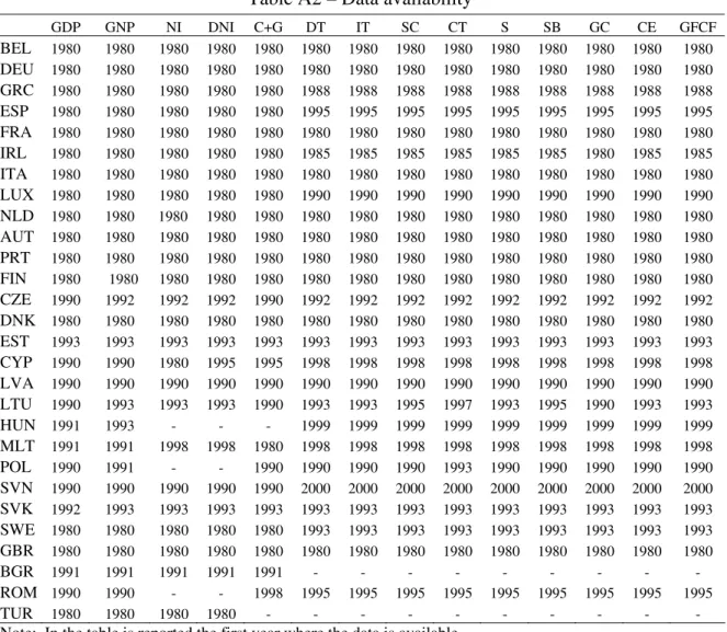
Table A2 – Data availability

GDP GNP NI DNI C+G DT IT SC CT S SB GC CE GFCF

BEL 1980 1980 1980 1980 1980 1980 1980 1980 1980 1980 1980 1980 1980 1980

DEU 1980 1980 1980 1980 1980 1980 1980 1980 1980 1980 1980 1980 1980 1980

GRC 1980 1980 1980 1980 1980 1988 1988 1988 1988 1988 1988 1988 1988 1988

ESP 1980 1980 1980 1980 1980 1995 1995 1995 1995 1995 1995 1995 1995 1995

FRA 1980 1980 1980 1980 1980 1980 1980 1980 1980 1980 1980 1980 1980 1980

IRL 1980 1980 1980 1980 1980 1985 1985 1985 1985 1985 1985 1980 1985 1985

ITA 1980 1980 1980 1980 1980 1980 1980 1980 1980 1980 1980 1980 1980 1980

LUX 1980 1980 1980 1980 1980 1990 1990 1990 1990 1990 1990 1990 1990 1990

NLD 1980 1980 1980 1980 1980 1980 1980 1980 1980 1980 1980 1980 1980 1980

AUT 1980 1980 1980 1980 1980 1980 1980 1980 1980 1980 1980 1980 1980 1980

PRT 1980 1980 1980 1980 1980 1980 1980 1980 1980 1980 1980 1980 1980 1980

FIN 1980 1980 1980 1980 1980 1980 1980 1980 1980 1980 1980 1980 1980 1980

CZE 1990 1992 1992 1992 1990 1992 1992 1992 1992 1992 1992 1992 1992 1992

DNK 1980 1980 1980 1980 1980 1980 1980 1980 1980 1980 1980 1980 1980 1980

EST 1993 1993 1993 1993 1993 1993 1993 1993 1993 1993 1993 1993 1993 1993

CYP 1990 1990 1980 1995 1995 1998 1998 1998 1998 1998 1998 1998 1998 1998

LVA 1990 1990 1990 1990 1990 1990 1990 1990 1990 1990 1990 1990 1990 1990

LTU 1990 1993 1993 1993 1990 1993 1993 1995 1997 1993 1995 1990 1993 1993

HUN 1991 1993 - - - 1999 1999 1999 1999 1999 1999 1999 1999 1999

MLT 1991 1991 1998 1998 1980 1998 1998 1998 1998 1998 1998 1998 1998 1998

POL 1990 1991 - - 1990 1990 1990 1990 1993 1990 1990 1990 1990 1990

SVN 1990 1990 1990 1990 1990 2000 2000 2000 2000 2000 2000 2000 2000 2000

SVK 1992 1993 1993 1993 1993 1993 1993 1993 1993 1993 1993 1993 1993 1993

SWE 1980 1980 1980 1980 1980 1993 1993 1993 1993 1993 1993 1993 1993 1993

GBR 1980 1980 1980 1980 1980 1980 1980 1980 1980 1980 1980 1980 1980 1980

BGR 1991 1991 1991 1991 1991 - - - -

ROM 1990 1990 - - 1998 1995 1995 1995 1995 1995 1995 1995 1995 1995

TUR 1980 1980 1980 1980 - - - -

Note: In the table is reported the first year where the data is available. (-) means missing.

References

Alesina, A. and Barro, R. (2002). “Currency unions”, Quarterly Journal of Economics

117, 409-436.

Alesina, A.; Barro, R. and Tenreyro, S. (2002). “Optimal currency areas”, NBER Working Papers, 9072.

Alesina, A. and Wacziarg, R. (1999). "Is Europe Going too Far?” Carnegie-Rochester

Conference Series on Public Policy, 51, 1-42.

Alesina, A. and Grilli, V. (1992). "The European Central Bank: Reshaping Monetary Politics in Europe," In M.B.Canzoneri, V.Grilli, and P.R.Masson (eds.) Establishing a

Central Bank: Issues in Europe and Lessons from the U.S., Cambridge.

Angeloni, I. and Dedola, L. (1999). “From the ERM to the Euro: nee evidence on economic and policy convergence among EU countries”, European Central Bank Working Paper 4.

Arreaza, M; Sorensen, B. and Yosha, O. (1998). “Consumption Smoothing through Fiscal Policy in OECD and EU Countries,” NBER Working Papers No. 6372.

Artis, M. and Zhang, W. (1997). “International business cycles and the ERM: Is there a European business cycle,” International Journal of Finance and Economics, 2 (1), 1-16.

Artis, M., Marcellino, M., Proietti, T. (2004). “Characterising the business cycles for accession countries”, CEPR Discussion Paper No. 4457.

Asdrubali, P.; Sorensen, B. and Yosha, O. (1996). “Channels of Interstate Risk Sharing: United States 1963-90”, Quarterly Journal of Economics, 111, 1081-1110.

Bayoumi, T. and Prasad, E. (1997) “Currency Unions, Economic Fluctuations, and Adjustment: Some New Empirical Evidence”, IMF Staff Papers, 44 (1), 36-57.

Barro, R. and Gordon. D. (1983). “Rules, Discretion and Reputation in a Model of Monetary Policy”. Journal of Monetary Economics, 12, 101-122.

Baxter, M. and King, R. (1999). “Measuring Business Cycles: Approximate Band-Pass Filters for Economic Time Series”, Review of Economics and Statistics, 81 (4), 575-593.

Christiano, L. and Fitzgerald, T. (2003). “The Band Pass Filter,” International Economic

Review, 4 (2), 435-465.

Corsetti, G. and Pesenti, P. (2002) “Self-validating optimum currency areas,” NBER Working Papers, 8783.

Fatás, A. (1997). “EMU: countries or regions: lessons from the EMS experience,”

European Economic Review, 41 (3-5), 743-751.

Fidrmuc, J. (2001) “The endogeneity of the optimum currency area criteria, intraindustry trade, and EMU enlargement”. Discussion Paper No. 106/2001. Centre for Transition Economics, Katholieke Universiteit, Leuven.

Fidrmuc, J. (2004). “The endogeneity of the optimum currency area criteria, intra-industry trade, and EMU enlargement”, Contemporary Economic Policy 22, 1-12.

Fidrmuc, J. and Korhonen, I. (2006). “Meta-Analysis of the Business Cycle Correlation between the Euro Area and the CEECs,” CESifo Working Paper No. 1693.

Furceri, D. and Karras, G. (2006). ”Business Cycle Synchronization in the EMU”, Applied

Economics (forthcoming).

Frankel, J. and Rose, A. (1998). “The Endogeneity of the Optimum Currency Area Criteria,” Economic Journal 108, 1009-1025.

Giannone, D. and Reichlin, L. (2006). “Trends and cycles in the euro area: how much heterogeneity and should we worry about it?” European Central Bank, Working Paper N. 595.

Goodhart, C. and Smith, S. (1993) ‘Stabilization’, European Economy, Reports and Studies, 5, 417-56.

Hammond, J. and von Hagen, J. (1995)“Regional Insurance Against Asymmetric Shocks: An Empirical Study for The European Community,” Manchester School, 66, 331-53.

Hodrick, R. and Prescott, E. (1980) “Postwar U.S. Business Cycles: An Empirical Investigations”, Discussion Papers 451, Carnegie Mellon University.

Karras, G. (2002). “Costs and Benefits of Dollarization: Evidence from North, Central, and South America”, Journal of Economic Integration, 17 (3), 502-516.

Kenen, R. (1969) “The theory of optimum currency area:an eclectic view,” in: R. Mundell and A. Swoboda, (eds.), Monetary problems of the international economy, Chicago, Univeristy of Chicago Press.

Kydland, F. and Prescott. E. (1977). ”Rules Rather Than Discretion: The Inconsistency of Optimal Plans,” Journal of Political Economy, 85, 473-490.

Masson, P. and Taylor, M. (1992). “Common Currency Areas and Currency Unions: An Analysis of the Issues,” CEPR Discussion Paper, 617.

Maurel, M. (2002). “On the way of EMU enlargement towards CEECs: What is the appropriate exchange rate regime?” CEPR Discussion Paper No. 3409.

Mélitz, J. and Zumer, F. (2002). “Regional Redistribution and Stabilization by theCentral Governement in Canada, France, the UK and the US: A Reassessment and New Tests,”

Journal of Public Economics, 86 (2), 263-286.

Mundell, R. (1961) “A theory of optimum currency areas,” American Economic Review, 82, 942-963.

Obstfeld, M. and Peri, G. (1998). “Regional Non-Adjustment and Fiscal Policy,” Economic

Policy, April, 207-59.

Ravn, M. and Uhlig, H. (2002). “On Adjusting the Hodrick-Prescott Filter for the Frequency of Observations”. Review of Economics and Statistics, 84 (2), 371-380.

Rose, A. and Stanley, T. (2005) “A meta analysis of the effect of common currencies on international trade,” Journal of Economic Surveys, 19 (3), 347-365.

Rose, A. and Engel, C. (2002). “Currency unions and international integration,” Journal of

Money, Credit and Banking 34, 1067-1089.

Sachs, J. and Sala-i-Martin, X. (1991).“Fiscal Federalism and Optimum Currency Areas: Evidence for Europe from The US,” NBER Working Paper, 3885

Sorensen, B. and Yosha, O. (1998). “International Risk Sharing and European Monetary Unification”, Journal of International Economics, 45, 211-238.

Stock, J. and Watson, M. (1999). “Business Cycle Fluctuations in U.S. Macroeconomic Time Series”, in Taylor, J. and Woodford, M. (eds.), Handbook of Macroeconomics, vol 1, 3-64, Elsevier.

Tables and Figures

Table 1 – Business cycle synchronisation (vis-à-vis EMU)

HP6.25 1980-1992 1993-2005 1980-2005

EMU

Austria 0.534 0.793 0.647

Belgium 0.692 0.832 0.762

Finland 0.582* 0.478 0.509*

France 0.615 0.977 0.786

Germany 0.763 0.678 0.696

Greece 0.601 0.441 0.554

Ireland 0.285 0.645 0.465

Italy 0.539 0.810 0.674

Luxembourg 0.419 0.745 0.570

Netherlands 0.542 0.875 0.692

Portugal 0.341 0.733 0.507

Spain 0.506 0.871 0.662

Other EMU

Czech Republic 0.031

Denmark 0.043 0.569 0.258

Estonia -0.220

Cyprus 0.541

Latvia 0.238

Lithuania -0.032

Hungary 0.789

Malta 0.698

Poland 0.247

Slovenia 0.412

Slovakia -0.673

Sweden 0.164 0.695 0.443

UK -0.137 0.594 0.042

Candidate countries

Bulgaria 0.342

Romania -0.242

Turkey -0.273

Note: HP6.25=Hodrick-Prescott Filter with smoothness parameter equal to 6.25.

Table 2 – Channel of output smoothing (GLS)

EMU EU 15 EU 25^

1980-2005 1992-2005 1998-20051980-2005 1992-2005 1998-2005 1992-2005 1998-2005

Factor Income ( βm) 1.07 6.64** 13.64*** -0.25 4.98* 11.78*** -0.39 6.44 (0.48) (2.29) (2.85) (-0.13) (1.88) (2.58) (-0.31) -2.87 [300] [168] [96] [375] [210] [120] [315] [184] -6.30*** -2.46* -2.20 -7.58*** -3.05** -2.81 -3.81 -9.26 (-4.04) (-1.85) (-1.05) (-5.67) (-2.45) (--1.47) (-1.64)* (-5.77) Capital

Depreciation ( βd)

[300] [168] [96] [375] [210] [120] [308] [183] 2.14 -1.09 1.34 2.39** _{-0.79 1.59 -2.7}* _0.97

(1.53) (-0.47) (0.54) (2.13) (-0.40) (0.71) (-1.93) -0.75 International

Transfers ( βg₎

[300] [168] [96] [368] [210] [120] [303] [183] Saving ( βs_{) 39.01}*** _50.43*** _24.79*** _36.86*** _50.71*** _25.21*** _38.12*** _34.46***

(6.50) (6.21) (2.62) (6.97) (6.83) (2.86) (5.74) (5.36) [300] [168] [96] [368] [210] [120] [298] [182] Not Smoothed ( βu_{) 56.83}***

49.93*** 63.43*** 61.12*** 50.19*** 62.72*** 63.97*** 69.37*** (11.68) (10.52) (11.25) (14.11) (10.98) (10.46) (5.90) (15.61) [300] [168] [96] [375] [210] [120] [302] [182]

Notes: Fraction of shocks (percentage points) absorbed at each level of smoothing. T-statistics are in parenthesis and the number of observations in square brackets.

*, **, *** - statistically significant at the 10, 5, and 1 percent level respectively.

m

β is the two-step GLS estimate of the slope in the regression of ∆logGDP−∆logGNP on

GDP

log

∆ , βd is the slope in the regression of ∆logGNP−∆logNI on ∆logGDP, βg is the slope in the regression of ∆logNI −∆logDNI on ∆logGDP, βs is the slope in the regression of

(

)

DNI −∆ +

∆log log on ∆logGDP, and finallyβu is the slope in the regression of

(

)

DNI −∆ +

∆log log on ∆logGDP. We interpret the β coefficients as the incremental percentage amounts of smoothing achieved at each level. And thus βu is the amount of shock not smoothed. The sum of the coefficient could not sum to 100 percent due to rounding, due the fact that for some regression we have an unbalanced panel and that our estimates are GLS.

^

Table 3 – Fiscal Channels of output smoothing (GLS)

EMU EU 15 EU 25^

1980-2005 1992-2005 1998-2005 1980-2005 1992-2005 1998-2005 1992-2005 1998-2005 Direct Taxes -4.21 -4.21 -3.16 -3.12 -3.72 -2.08 -4.27* -0.21 (-1.38) (-1.37) (-0.80) (-1.04) (-1.23) (-0.54) (-1.88) (-0.08) [262] [164] [96] [317] [204] [120] [287] [182] Indirect Taxes -3.23* -2.44 2.42 -2.62 -2.89 1.39 -3.10* 0.78 (-1.71) (-1.06) (-0.71) (-1.44) (-1.32) (0.41) (-1.63) (0.03) [262] [164] [96] [317] [204] [120] [287] [182] -5.49*** -4.69** 5.04** -4.10*** -4.00** 3.52 -5.51*** -1.31 (-3.15) (-2.33) (2.08) (-2.64) (-2.20) (1.58) (-3.60) (-0.68) Social

Contributions

[262] [164] [96] [317] [204] [120] [287] [182] Capital Taxes -0.21 -0.14 -0.85 -0.01 -0.05 -0.07 -0.04 -0.17 (-0.93) (-0.44) (-0.25) (-0.75) (-0.19) (-0.26) (-0.25) (-0.49) [262] [164] [96] [317] [204] [120] [287] [182] Subsides 0.94 -0.24 -0.21 0.11* _{-0.31 -0.04 -0.74 1.37}

(1.21) (-.042) (-0.37) (1.63) (-0.53) (-0.71) (-1.51) (0.26) [262] [164] [96] [317] [204] [120] [287] [182] Social Benefits 7.39*** _6.27*** _6.31** _9.09*** _6.98*** _7.47*** _7.81*** _9.11***

(4.02) (3.07) (2.47) (5.11) (3.42) (3.03) (5.16) (4.27) [262] [164] [96] [317] [204] [120] [287] [182] 3.42* 2.30 3.89 6.24*** 4.35** 4.89* 8.31*** 8.22*** (1.82) (1.13) (1.25) (3.50) (2.14) (1.63) (3.82) (3.29) Government

Consumption

[262] [164] [96] [317] [204] [120] [287] [182] 2.09* 1.36 -0.64 3.59*** 2.56** 0.07 5.91*** 5.45*** (1.91) (1.25) (-0.34) (3.31) (2.24) (0.40) (4.92) (3.45) Compensation of

Employees

[262] [164] [96] [317] [204] [120] [287] [182] -2.21** -1.88 -5.72*** -2.29** -1.82 -5.45*** 0.15 -3.81*** (-2.23) (-1.61) (-3.51) (-2.39) (-1.55) (-3.27) (0.19) (-3.18) Gross Fixed

Capital

Formation [262] [164] [96] [401] [204] [120] [287] [182]

Notes: Fraction of shocks (percentage points) absorbed at each level of smoothing. T-statistics are in parenthesis and the number of observations in square brackets.

*, **, *** - statistically significant at the 10, 5, and 1 percent level respectively.

^

Figure 1 – Business Cycle Synchronization vis-à-vis the EMU (1980-2005)

Business Cycle Syncronization EU15 (nine-years rolling windows estimation)

-0.8 -0.6 -0.4 -0.2 0.0 0.2 0.4 0.6 0.8 1.0

1 2 3 4 5 6 7 8 9 10 11 12 13 14 15 16 17 18

Time

Corre

la

ti

ons

BEL DEU GRC ESP FRA IRL IT A LUX

NLD AUT PRT FIN DNK SWE GBR

Note: each period is nine years long. 1=1980-1988, 2=1981-1989,…, 18=1997-2005.

Figure 2 – Business Cycle Synchronization vis-à-vis the EMU (1992-2005)

Business Cycle Syncronization new EU and candidate (nine-years rolling windows estimation)

-1.0 -0.8 -0.6 -0.4 -0.2 0.0 0.2 0.4 0.6 0.8 1.0

1 2 3 4 5 6

Time

Corre

la

ti

ons

CZE EST CYP LVA LT U HUN MLT

POL SVN SVK BGR ROM T UR

Appendix 1 – Additional Results

Table A1 – Spearman’s rank correlation matrix

HP6.25 HP100 BP Diff

HP6.25 1.000

HP100 0.936 1.000 BP 0.847 0.855 1.000

Diff 0.839 0.776 0.788 1.000

Table A2 - Channel of output smoothing (OLS)

EMU EU 15 EU 25^

1980-2005 1992-2005 1998-2005 1980-2005 1992-2005 1998-2005 1992-2005 1998-2005

Factor Income ( βm_{) 7.79 12.67}*

23.46*** 6.22 11.56* 23.68*** -1.16 10.64*** (1.35) (1.93) (3.06) 1.20) (1.81) (3.25) (-0.28) (3.03) [300] [168] [96] [375] [210] [120] [315] [184] -6.85* -1.95 -1.36 -7.39** -2.33 -0.28 8.17 -12.25*** (-1.93) (-0.94) (-0.09) (-2.39) (-1.07) (-0.17) 0.51 (-3.05) Capital

Depreciation ( βd₎

[300] [168] [96] [375] [210] [120] [308] [183]

-3.49 -12.43 -10.55 -2.49 -11.75 -10.23 -8.17** _-3.68

(-0.77) (-1.39) (-0.93) (-0.65) (-1.39) (-0.93) (-2.43) (-0.95) International

Transfers ( βg₎

[300] [168] [96] [368] [210] [120] [303] [183]

Saving ( βs) 47.12*** 51.75** 23.72** 44.38*** 51.63*** 22.96** 43.04 32.80*** (6.23) (2.88) (2.60) (6.34) (2.90) (2.60) (1.00) (5.63) [300] [168] [96] [368] [298] [120] [298] [183] Not Smoothed ( βu) 55.43*** 49.96*** 63.50*** 59.68*** 50.89*** 63.87*** 41.72 72.40*** (11.89) (7.57) (12.28) (10.68) (7.83) (13.45) (0.59) (16.06) [300] [168] [96] [375] [210] [120] [302] [184]

Notes: Fraction of shocks (percentage points) absorbed at each level of smoothing. T-statistics are in parenthesis and the number of observations in square brackets. Robust standard errors for Heteroskedasticity and AR (1). *, **, *** - statistically significant at the 10, 5, and 1 percent level respectively.

m

β is the OLS estimate of the slope in the regression of ∆logGDP−∆logGNP on ∆logGDP, βd is the slope in the regression of ∆logGNP−∆logNI on ∆logGDP, βg is the slope in the

regression of ∆logNI −∆logDNI on ∆logGDP, βs is the slope in the regression of

(

)

DNI −∆ +

∆log log on ∆logGDP, and finallyβu is the slope in the regression of

(

)

DNI −∆ +

∆log log on ∆logGDP. We interpret the β coefficients as the incremental percentage amounts of smoothing achieved at each level. And thus βu is the amount of shock not smoothed. The sum of the coefficient could not sum to 100 percent due to rounding, due the fact that for some regression we have an unbalanced panel.

^

Table A3 – Fiscal Channels of output smoothing (OLS)

EMU EU 15 EU 25^

1980-2005 1992-2005 1998-2005 1980-2005 1992-2005 1998-2005 1992-2005 1998-2005 Direct Taxes -4.94** -2.76 -4.74 -3.49 -1.75 -2.02 -6.11** -0.21 (-2.23) (-0.88) (-0.91) (-1.55) (-0.57) (-0.36) (-2.75) (-0.08) [270] [164] [96] [317] [204] [120] [287] [182] Indirect Taxes -3.75* -1.99 -3.19 -2.73 -2.07 -2.67 -4.27** -2.55 (-1.83) (-0.60) (-0.76) (1..27) (-0.66) (-0.68) (-2.21) (-0.87) [262] [164] [96] [317] [204] [120] [287] [182]

-5.95 -3.10 5.82 -5.59 -3.63 4.33 -8.96*** -3.73 (-1.69) (-1.24) (1.86) (-1.72) (-1.47) (1.51) (-4.96) (-1.51) Social

Contributions

[262] [164] [96] [317] [204] [120] [287] [182] Capital Taxes -0.33 -0.54 0.53 -0.18 0.01 0.44 0.14 0.05 (-0.94) (-0.11) (0.64) (-0.68) (0.19) (0.60) (0.63) (0.16) [262] [164] [96] [317] [204] [120] [287] [182] Subsides 1.52 0.31 0.58 1.61 -0.01 0.23 -1.52 1.41** (1.21) (0.46) (0.94) (1.47) (-0.17) (0.45) (-1.40) (2.48) [262] [164] [96] [317] [204] [120] [287] [182] Social Benefits 10.90 8.09 4.38* 11.35* 7.44 3.91* 9.26*** 9.91*** (1.72) (1.59) (1.96) (2.06) (1.55) (1.71) (7.10) (4.31) [262] [164] [96] [317] [204] [120] [287] [182] 6.62 3.48 2.82 7.55* 4.28 3.31 14.91*** 10.43*** (1.65) (1.34) (0.77) (2.08) (1.65) (0.99) (4.87) (3.62) Government

Consumption

[262] [164] [96] [317] [204] [120] [287] [182] 3.85 1.38 -1.98 4.76 2.30 -0.94 8.38*** 5.47*** (1.23) (1.13) (-0.94) (1.68) (1.73) (0.44) (5.52) (3.02) Compensation of

Employees

[262] [164] [96] [317] [204] [120] [287] [182] -2.47** -2.48 -4.69*** -2.78** -2.67 -3.92** 1.09 -2.74*** (-2.22) (-1.51) (-4.33) (-2.49) (-1.61) (-2.64) (0.86) (-2.95) Gross Fixed

Capital Formation

[262] [164] [96] [317] [204] [120] [287] [182] Notes: Fraction of shocks (percentage points) absorbed at each level of smoothing. T-statistics are in parenthesis and the number of observations in square brackets. Robust standard errors for Heteroskedasticity and AR (1).

*, **, *** - statistically significant at the 10, 5, and 1 percent level respectively.

^