Modelling of volumetric solar receivers with nanoparticle suspensions

UNIVERSITY OF ÉVORA

SCHOOL OF SCIENCE AND TECHNOLOGY

DEPARTMENT OF PHYSICS

Modelling of volumetric solar receivers with

nanoparticle suspensions

Tiago Emanuel Ramos Tidy

Supervision: Paulo Manuel Ferrão Canhoto, Ph.D.

Masters in Solar Energy Engineering

Dissertation

UNIVERSITY OF ÉVORA

SCHOOL OF SCIENCE AND TECHNOLOGY

DEPARTMENT OF PHYSICS

Modelling of volumetric solar receivers with

nanoparticle suspensions

Tiago Emanuel Ramos Tidy

Supervision: Paulo Manuel Ferrão Canhoto, Ph.D.

Masters in Solar Energy Engineering

Dissertation

“You never change things by fighting the existing reality. To change something, build a new model that makes the existing model obsolete.“ R. Buckminster Fuller

i

A

I would like to express my gratitude to all who have directly or indirectly contributed in putting together this dissertation.

Firstly, I would like to express my sincere thanks and gratitude to my supervisor, Professor Paulo Canhoto, for his mentoring and feedback. The motivation he gave me to challenge myself and overcome many barriers must be recognized. I also acknowledge his constant availability, incentive and collaboration provided to this project, making these last few months an unforgettable experience.

I also gratefully thank the University of Évora and its Geophysics Centre for providing the space and necessary materials for this dissertation. The contribution of Sérgio Aranha from the physics department was of course invaluable and I am very grateful for the time and interest he invested in this project. Special thanks to Josué Figueira for all his dedication on the manufacturing and assembly of parts of the experimental apparatus. Dr. Miguel Potes also provided important equipment and helpful input and advice on the spectroradiometer functioning. I also thank Maria Helena from the chemistry department for providing indispensable equipment and for sharing her chemistry knowledge in the nanotechnology field.

I am very thankful to all my colleagues who shared the lab space with me, especially Germilly Barreto for helping me and motivating me to work harder and harder. I owe my sincere appreciation to my classmates and friends, who have supported, encouraged and guided me throughout my academic life. I would like to particularly thank Carlos Sousa for his truthful friendship and Cláudia Franco for her unconditional support and advice.

Finally, I would like to express my deepest gratitude to my family, in particular to my parents, for their extraordinary support and constant encouragement.

iii

A

This work addresses the modelling of nanofluid-based volumetric receivers aiming the improvement of solar energy harvesting and conversion systems. A numerical heat transfer model (1-D) was developed to predict the energy gain in a non-flowing receiver, in which both receiver height and particles volume fraction were optimized. Various combinations of base fluids (water, mineral oils, ethylene glycol) and nanoparticles (graphite, carbon nanotubes) were considered by modelling their optical and thermodynamic properties. Specific characteristics and advantages of volumetric receivers were emphasized by comparing numerical results with those obtained for a surface-based receiver, and by experimental measurements. A two-dimensional numerical model was also developed to investigate the performance of a parallel plate volumetric receiver with a fully developed laminar flow under various operation conditions. It was found that a better performance was obtained when using solid particles of carbon nanotubes.

Keywords: Volumetric, direct absorption, nanofluid, volume fraction, performance, temperature

v

R

Modelação de recetores solares volúmicos com nanopartículas suspensas

Este trabalho aborda a modelação de recetores volúmicos com nanofluidos tendo como objetivo o melhoramento de sistemas de captação e conversão de energia solar. Foi desenvolvido um modelo numérico de transferência de calor unidimensional para prever a energia ganha num recetor estagnado, onde a altura e a fração volúmica de partículas foram otimizadas. Várias combinações de fluidos (água, óleos minerais, etileno glicol) e nanopartículas (grafite, nanotubos de carbono) foram consideradas através da modelação das suas propriedades óticas e radiativas. As características específicas e vantagens dos recetores volúmicos foram destacadas através da comparação dos resultados numéricos com os obtidos num recetor de superfície, e através de medidas experimentais. Foi também desenvolvido um modelo numérico bidimensional para investigar o desempenho de um receptor volúmico com escoamento laminar e plenamente desenvolvido entre placas paralelas, sob várias condições de operação. Verificou-se que o melhor desempenho foi obtido usando partículas sólidas de nanotubos de carbono.

Palavras-Chave: Volumétrico, absorção direta, nanofluido, fração volúmica, desempenho, perfil de

vii

C

1.2. Outline of the dissertation ... 5

2. Nanofluid preparation and properties ... 7

2.1. Preparation and stability ... 7

2.2. Thermodynamic and transport properties ... 9

2.3. Radiative properties ... 11

2.3.1. Experimental characterization of radiative properties ... 12

3. Nanofluid-based receiver modelling and optimization ... 15

3.1. Volumetric heat rate profile ... 16

3.1.1. Absorption efficiency ... 17 3.2. Temperature profile ... 17 3.3. Numerical model ... 18 3.3.1. Internal plane ... 20 3.3.2. Boundary conditions ... 21 3.4. Receiver efficiency ... 23 3.5. Numerical results ... 23

3.5.1. Heat release profile ... 24

3.5.2. Temperature profile ... 28

4. Comparison between surface-based and nanofluid-based receivers ... 35

4.1. Surface-based receiver modelling ... 35

4.2. Comparison of results ... 42

5. Experimental study on nanofluids ... 45

5.1. Equipment characteristics ... 45

5.1.1. Datalogger ... 45

viii 5.1.3. Pyranometer ... 49 5.1.4. Volumetric receiver ... 50 5.1.5. Solar simulator ... 51 5.2. Nanofluid ... 56 5.2.1. Nanofluid properties ... 56 5.2.2. Nanofluid preparation ... 58

5.3. Results and experimental validation ... 59

6. Modelling of a volumetric flow receiver ... 63

6.1. Temperature profile ... 63 6.2. Numerical model ... 64 6.2.1. Internal points ... 66 6.2.2. Boundary points ... 67 6.3. Receiver efficiency ... 68 6.4. Numerical results ... 68

7. Conclusions and future work ... 75

8. References ... 77

ix

L

F

Figure 1.1 – Temperature profile of a volumetric (a) and a surface-based receiver (b) [2] ... 2

Figure 2.1 – Spectrum of ASD Pro-lamp... 13

Figure 2.2 – Experimental setup for a transmissivity measurement ... 14

Figure 2.3 – Transmissivity of pure water [29] and Perfecto HT 5 thermal oil ... 14

Figure 3.1 – Schematic for model formulation of a volumetric solar receiver ... 15

Figure 3.2 – Comparison between AM0, AM1.5 Global and AM1.5 Direct spectra [30] ... 17

Figure 3.3 – One-dimensional mesh on a volumetric receiver ... 18

Figure 3.4 – One-dimensional mesh for internal plane on a volumetric receiver ... 20

Figure 3.5 – One-dimensional mesh for top plane on a volumetric receiver ... 21

Figure 3.6 – One-dimensional mesh for bottom plane on a volumetric receiver ... 22

Figure 3.7 – Heat release profile (H = 0,01 m; fv = 0,01%) ... 24

Figure 3.8 – Effect of volume fraction on absorption efficiency ... 26

Figure 3.9 – Dimensionless heat release profile for different heights ... 27

Figure 3.10 – Effect of receiver height on absorption efficiency ... 28

Figure 3.11 – Temperature profile in transient regime for a graphite-based receiver ... 29

Figure 3.12 – Temperature profile in transient regime for a MWCNT-based receiver ... 29

Figure 3.13 – Coloured temperature profile in transient regime for a MWCNT-based receiver ... 30

Figure 3.14 – Variation of maximum temperatures with different concentration factors for a graphite-based receiver ... 31

Figure 3.15 – Variation of maximum temperatures with different concentration factors for a MWCNT-based receiver ... 31

Figure 3.16 – Variation of accumulated values of energy gain and loss ... 32

Figure 3.17 – Variation of efficiency on different nanofluids ... 33

Figure 4.1 – Schematic for model formulation of a surface-based solar receiver ... 35

Figure 4.2 – One-dimensional mesh for top plane on a surface-based receiver ... 36

Figure 4.3 – Temperature profile on transient regime for a selective surface-based receiver... 37

Figure 4.4 – Three-dimensional temperature profile on transient regime for a selective surface-based receiver ... 38

Figure 4.5 – Variation of maximum temperatures with different concentration factors ... 39

Figure 4.6 – Variation of accumulated values of energy gain and energy loss ... 39

Figure 4.7 – Variation of efficiency on different fluids ... 40

Figure 4.8 – Variation of temperature on transient regime for a surface-based receiver ... 42

Figure 4.9 – Variation of temperature on transient regime for a nanofluid-based receiver ... 43

Figure 5.1 – Schematic of the experimental setup ... 45

Figure 5.2 – CR10 Datalogger [35] ... 46

Figure 5.3 – Thermocouple (type T) ... 47

Figure 5.4 – Connection diagram of a 3 wire half bridge configuration of a PT100 [34] ... 47

Figure 5.5 – Eppley 8-48 pyranometer [37] ... 49

x

Figure 5.7 – Volumetric receiver ... 50

Figure 5.8 – Spectrum of the extraterrestrial solar radiation compared to the spectrum of a 5777 K blackbody ... 51

Figure 5.9 – Comparison between AM0, AM1.5 Direct and solar simulator spectral distribution ... 53

Figure 5.10 – MWCNT structure [42] ... 56

Figure 5.11 – Transmissivity of the different nanofluids ... 57

Figure 5.12 – Sonicating bath ... 58

Figure 5.13 – Fluid samples used in the experimental apparatus ... 59

Figure 5.14 – Experimental setup ... 59

Figure 5.15 – Spectrum of the lamp for solar simulator in the experimental setup ... 60

Figure 5.16 – Comparison of experimental and numerical results for graphite + water nanofluid .. 61

Figure 5.17 – Comparison of experimental and numerical results for MWCNT + Perfecto HT 5 nanofluid... 62

Figure 6.1 – Schematic for model formulation of a nanofluid-based solar receiver ... 63

Figure 6.2 – Bi-dimensional mesh for receiver domain discretization ... 65

Figure 6.3 – Velocity profile between parallel plates ... 65

Figure 6.4 – Flowchart of the numerical model formulation ... 66

Figure 6.5 – Boundary conditions schematic ... 67

Figure 6.6 – Temperature profile in transient regime at different points of the receiver length ... 69

Figure 6.7 – Mean outlet temperature under different solar concentration factors... 69

Figure 6.8 – Mean outlet temperature for different nanofluids ... 70

Figure 6.9 – Efficiency of the volumetric flow receiver for different nanofluids ... 71

Figure 6.10 – Velocity impact on the receiver outlet temperature for different solar concentration factors ... 72

Figure 6.11 – Inlet temperature impact on the outlet temperature for different nanofluids ... 72

Figure 6.12 – Inlet temperature impact on the receiver efficiency for different nanofluids ... 73

Figure 6.13 – Inlet temperature impact on the receiver efficiency for different radiation levels .... 73

Figure 6.14 – Temperature profile in transient regime at different points of the receiver length ... 74

Figure 9.1 – Refractive index (n) and extinction coefficient (σ) of graphite [46] ... 83

Figure 9.2 – Extinction coefficient (σ) of Therminol VP1 [47] ... 83

Figure 9.3 – Transmissivity (𝝉) of Therminol VP1 using Eq. (2.11) ... 83

Figure 9.4 – Refractive index (n) and extinction coefficient (σ) of water [29] ... 84

Figure 9.5 – Transmissivity (𝝉) of water using Eq. (2.11) ... 84

Figure 9.6 – Refractive index (n) of ethylene glycol [48] ... 84

Figure 9.7 – Extinction coefficient (σ) of ethylene glycol [47] ... 85

Figure 9.8 – Transmissivity (𝝉) of ethylene glycol using Eq. (2.11) ... 85

Figure 9.9 – Print screen of the RS3 software for spectophotograms collection ... 86

Figure 9.10 – Function for volume fraction optimization through the Newton method ... 89

Figure 9.11 – Newton’s method implementation ... 90

Figure 9.12 – Programming window of CR10 ... 92

xi

L

T

Table 2.1 – Thermodynamic properties of liquids ... 10

Table 2.2 – Thermodynamic properties of solids ... 10

Table 2.3 – Dynamic Viscosity of liquids ... 10

Table 3.1 – Comparison between absorption efficiency for different nanofluids (H = 0,01 m; fv = 0,01%) ... 25

Table 3.2 – Numerical error for different nanofluids (H = 0,01 m; fv = 0,01%) ... 25

Table 3.3 – Optimum volume fraction for 99,99% absorption efficiency (H = 1 cm; Δy = 0,006 cm)26 Table 3.4 – Numerical error for different nanofluids (H = 1 cm; Δy = 0,006 cm; ƞabs = 99,99%) ... 27

Table 3.5 – Maximum temperature for different solar concentration factors (H = 1 cm; ƞabs = 99,99%; time = 1 hour) ... 30

Table 3.6 – Numerical error for different nanofluids for C = 1 ... 31

Table 3.7 – Receiver efficiency for different solar concentration factors (H = 1 cm; ƞabs = 99,99%; time = 1 hour) ... 33

Table 4.1 – Maximum temperatures for different concentration factors of a surface-based receiver ... 39

Table 4.2 – Comparison between fluids efficiency for different concentration factors for a surface-based receiver after 1 hour of operation ... 41

Table 5.1 – Classification criteria for spectral match ... 54

Table 5.2 – Spectral match classification for the solar simulator ... 54

Table 5.3 – Results for temporal instability of irradiance ... 55

xiii

N

𝐴 Area [m2_] 𝐵𝑖 Biot number [-]

𝑐_𝑝 Specific heat capacity [J/(kg K)] 𝐶 Solar concentration factor [-] 𝐷 Diameter [m]

𝑓_𝑣 Volume fraction of nanoparticles [m3_/m3_] 𝐹𝑜 Fourier number [-]

𝐺 Irradiance [W/m2_]

ℎ Heat transfer coefficient [W/(m2 _K)] 𝐻 Height [m]

𝐽_𝜆(𝑦) Spectral intensity [W/(m2 _nm)] 𝑘 Thermal conductivity [W/(m K)] 𝐿 Length [m]

𝑚 Relative refractive index [-] 𝑚̇ Mass flow rate [Kg/s] 𝑛 Refractive index [-] 𝑃𝑒 Péclet number [-] 𝑃𝑟 Prandtl number [-] 𝑃(𝑦) Radiative flux [W/m2_] 𝑞 Heat rate [W]

𝑞′′′ Volumetric heat rate [W/m3_] 𝑅 Resistance [Ω]

xiv t Time [s] T Temperature [°C] 𝑈 Wind speed [m/s] 𝑣 Velocity [m/s] 𝑉 Volume [m3_] 𝑉 Electric potential [V] Greek letters: 𝛼 Absorptivity [-] 𝛼 Thermal diffusivity [m2_/s] 𝜀 Emissivity [-] 𝜂 Efficiency [-] 𝜃 Angle [°] 𝜅 Absorption Coefficient [1/m] 𝜆 Wavelength [nm] 𝜇 Dynamic viscosity [kg/(m s)] 𝜌 Density [Kg/m3_] σ Extinction coefficient [-] σ Stefan–Boltzmann constant [W/(m2 _K4_)] 𝜏 Transmittance [-] Subscripts: 𝑎𝑏𝑠 absorption 𝑎𝑚𝑏 ambient 𝑐𝑜𝑛𝑣 convection

xv 𝑓 final ℎ hydraulic 𝑖 initial 𝑚𝑎𝑥 maximum 𝑟𝑎𝑑 radiation 𝑟𝑒𝑓 reference 𝑠𝑐𝑎𝑡 scattering Superscripts: ̅ average value ∗ dimensionless variable

xvii

A

AM Air Mass

ASTM American Society for Testing and Materials HTF Heat Transfer Fluid

IR Infrared

MWCNT Multi-Walled Carbon Nanotubes PRT Platinum Resistance Thermometer RTD Resistance Temperature Detectors TC Thermocouple

1

1. I

The shortage of fossil fuels, environmental concerns and increasing demand of energy shown in the past years make urgent the use of alternative energy sources. Renewable energies have proven to be a good and viable alternative since they are sustainable, free and abundant. In particular, efforts on the development of solar energy technologies have been made over the last years. One of the principal methods of harvesting and converting solar energy into thermal energy for subsequent use is through solar thermal collectors, which may vary drastically in their collecting and converting mechanisms. Nowadays, solar thermal technologies are used in a large variety of applications, such as water heating, electricity generation, drying, desalinization, etc. However, most of these technologies use an absorbing surface to harvest and convert solar radiation into thermal energy. This means that their efficiency is limited, not only by the absorber capability on capturing solar energy, but also by the quantity of energy (heat) that is transferred to a working fluid through conduction and convection. On one hand, selective coatings can be applied on the absorber surface in order to enhance absorptivity across the spectrum of incident solar radiation and decrease its emissivity in the thermal radiation spectrum. However, a thermal resistance is always present between the absorbing surface and the working fluid, resulting in a temperature difference between them, which is even bigger at high levels of solar concentration. This temperature difference leads to significant losses and therefore to lower conversion efficiencies.

On the other hand, and as an alternative, volumetric receivers can be used, in which solar radiation is directly absorbed in the volume of a nanofluid without directly heating any other structures within the receiver. A nanofluid is a fluid containing nanoparticles (nanometer-sized particles, usually 1 to 100 nm in diameter size [1]) suspended in a base fluid. Generally, the base fluid is transparent to solar radiation and the nanoparticles are responsible for the absorption and scattering of the incoming solar radiation passing through the medium. Since thermal conductivity of nanoparticles is substantially higher compared to the base fluid, absorbed energy is more uniformly distributed in the surrounding fluid, which decreases the temperature difference between the absorber particles and the base fluid.

Figure 1.1 illustrates the potential advantage of a volumetric receiver compared to an ideal selective surface, for the same mean fluid temperature (𝑇̅𝑓), incoming concentrated solar irradiance (𝐶𝐺𝑆) and height (𝐻). It is clear that the highest temperature occurs within the fluid in the direct

2

absorption solar collector (a), while for indirect absorption (b) the highest temperature occurs at the absorber surface, leading to higher emission losses [2].

Figure 1.1 – Temperature profile of a volumetric (a) and a surface-based receiver (b) [2]

According to M. A. Sadique and A. Verma [1] the use of nanofluids can increase the collector’s efficiency by 10% to 15%, yet, efficiency is still limited by the maximum allowable temperature of the heat transfer fluid (HTF). Depending on many factors, the performance of volumetric receivers may vary from these efficiency improvements. On this matter, O. Mahian et. al. [3] carried out a review on the different applications of nanofluids in solar energy, in which the assessment on the receiver performance obtained by each author is presented. One can highlight some of the state of the art developments:

A. Veeraragavan et. al. [4], developed an analytical model for the design of volumetric solar flow receivers and used graphite nanoparticles suspended in Therminol VP1 as a case of study. The volume fraction and receiver length were optimized where the total efficiency is maximized. Some similarities can be found in comparison to this dissertation, however, when calculating the heat release profile in the receiver, it was used the sun spectrum instead of the equivalent black body spectrum at 5800 K, and the optical properties of this nanofluid were modelled as a function of wavelengths, instead of using constant values. Also, a fully developed flow was considered in this dissertation as opposite to a plug flow.

To what concerns experimental apparatus, T. Otanicar et. al. [5] investigated the performance of graphite spheres, carbon nanotubes and silver spheres suspended in water as base fluid, on a micro-solar thermal collector. The authors demonstrated efficiency improvements up to 5% due to the influence of the nanofluid absorption mechanisms. A similar configuration to the one used on this dissertation was carried out by V. Khullar et. al. [6], in which amorphous carbon nanoparticles were

3

dispersed in ethylene glycol and multi-walled carbon nanotubes (MWCNTs) dispersed in distilled water. The authors also compared the obtained results with a solar selective surface-based receiver and concluded that higher stagnation temperatures were obtained with volumetric receivers. A. Lenert [7] also performed similar experiments to investigate the efficiency of nanofluid-based receivers for high temperature applications, such as power generation, using carbon-coated nanoparticles suspended in Therminol VP1. The results with nanofluids, considering the respective receiver design, suggested a major benefit for concentration levels superior to 100 and a receiver height superior to 10 cm.

In another way, studies regarding low temperature solar collectors have also been investigated, in which H. Tyagi and P. Phelan [8] compared the performance of two types of non-concentrating solar collectors: a typical flat-plate collector and a thin flowing film of nanofluid (mixture of water and aluminum nanoparticles). Under similar operating conditions the nanofluid-based receiver showed an increase of efficiency up to 10%. As an example of another low temperature configuration, R. Nasrin and M. A. Alim [9] investigated the heat transfer performance in a wavy solar collector, using silver and copper oxide nanoparticles suspended in water, in which the silver-based nanofluid performed the best.

A rather different approach to the one presented on this dissertation was developed by V. Khullar and H. Tyagi [10], in which an attempt to harvest solar energy through the usage of nanofluid-based concentrating parabolic solar collectors was carried out. A numerical model was implemented using the finite difference technique and results were compared with the experimental performance of conventional concentrating parabolic solar collectors under similar conditions. The authors concluded that a nanofluid-based collector with aluminum nanoparticles dispersed in Therminol VP1 improved efficiency in about 5 to 10%. No experimental study on this matter was found. Very recently, D. C. Hernandez Aita [11] developed a two-dimensional model to predict the temperature profile and performance of volumetric receivers using supercritical carbon dioxide as base fluid and carbon nanoparticles suspended in that medium. A comparison of this base fluid with Therminol VP1 was carried out for low inlet temperatures, in which the system performance improved 20%, and the outlet temperature increased approximately 250°C when using supercritical carbon dioxide. The optical thickness, receiver height and solar concentration factor parameters were optimized, which allowed to conclude that volumetric receivers have the potential to collect solar energy more efficiently when compared to surface-based receivers. However, surface-based

4

receivers with Therminol VP1 showed better system efficiencies for concentration factors lower than 7 and nanofluid height lower than 2,5 cm. The author also evaluated the performance of this technology when integrated into a Brayton cycle for concentrating solar plants. At a high inlet temperature of 675 K and considering an ideal Brayton cycle, the system proved to have potential to achieve efficiencies up to 68% for concentration factors higher than 30 and nanofluid height superior to 15 cm.

The developments carried out until now, have shown that volumetric receivers can be a more efficient way of collecting and converting solar energy. But how can these improvements be quantified as to the impact on the environment? Very few studies have been made on this matter. Concerning the non-concentrating technologies, T. Otanicar and J. Golden [12] demonstrated that in comparison to a conventional solar collector, the nanofluid-based receiver presents less emissions of carbon dioxide on both manufacturing and operating levels. As for the concentrating systems, V. Khullar and H. Tyagi [13] also showed considerable emission reductions and fuel savings if nanofluid-based concentration solar water heating systems are adopted.

In this dissertation, two different types of concentrating solar volumetric receivers were investigated. A first model under non-flowing conditions, in which the purpose was to study the temperature profile and performance of eight different nanofluids that result from a combination of two solid particles (graphite and MWCNTs) and four base fluids (water, Therminol VP1, Perfecto HT 5 and ethylene glycol). As part of this study, an experimental apparatus was prepared and results were compared with the numerical model. Similar temperature profiles were obtained which validated the numerical model. Under comparable operating conditions, the numerical model was also compared to a selective surface-based receiver to emphasize the different absorbing mechanisms of solar radiation. A second model was numerically developed in which the same nanofluids were tested under flowing conditions in a parallel plate geometry. An analysis on the impact of solar concentration factor, velocity and inlet temperature on such receiver was carried out.

5

1.1. Aim

The aim of this dissertation is to contribute to the development and optimization of volumetric receivers with nanoparticle suspensions. One of the main purposes of this work is to investigate the mechanisms that are responsible for sun light absorption due to nanofluids, and develop a numerical and experimental analysis under transient and stationary regimes of a solar receiver with stagnated fluid. A second objective is to improve the performance of volumetric flow receivers through the development of a numerical model for both transient and stationary conditions.

1.2. Outline of the dissertation

This dissertation is structured in seven distinct chapters organized as follows: In Chapter 1, a general introduction to the subject-matter is presented.

Chapter 2 introduces the nanofluids concept and features that allow enhancing the performance of volumetric receivers. A review on their preparation and stability issues is presented, and the radiative, thermal and transport properties are analyzed in detail.

Chapter 3 addresses the modelling of a non-flowing volumetric receiver in which only heat diffusion is considered. The volume fraction of nanoparticles is optimized to further determine the temperatures and efficiencies for eight different nanofluids under various conditions. Results are discussed and compared.

Chapter 4 concerns the comparison of the numerical results from Chapter 3 with those obtained for a surface-based receiver using a similar numerical model and considering four different fluids. Chapter 5 addresses an experimental study in which a volumetric receiver was designed and built. Four nanofluids were studied with the purpose of validating the numerical results of Chapter 3. Chapter 6 features the modelling of a volumetric flow receiver in which both diffusion and convection heat transfer are considered. An assessment of the receiver performance under different conditions is carried out for the same nanofluids studied in the previous chapters.

Finally, in Chapter 7, the main conclusions are presented and future work suggestions and improvements are proposed.

7

2. N

A nanofluid is composed by nanometer sized particles (usually 1 to 100 nm in diameter size [1]) suspended or dispersed in a fluid. Nanofluids have some uncommon features that give them a great potential on solar energy applications. Therefore, efforts for better understanding on how such fluids work should be made. The study of their preparation, stability and properties are of course a matter of concern, and will be analyzed in this chapter.

The enhancement on solar energy absorption by a nanofluid can be maximized with the change of particle size, shape, material and volume fraction. In respect to the material, different types of solid particles may be used in nanofluids [14]:

• Metals: Ag (silver), Al (aluminum), Au (gold), Cu (copper), Fe (iron).

• Oxides: Al2O3 (aluminum oxide), CuO or Cu2O (copper oxides), Fe2O3 (iron oxide), SiO2 (silicon dioxide), TiO2 (titanium dioxide).

• Carbon: graphite, single-walled nanotubes, double-walled nanotubes, or multi-walled carbon nanotubes.

• Other particles: Si (silicon) compounds

Concerning the most commonly used base fluids, they can be categorized as follows: • Liquids: water, organic and mineral fluids (such as thermal oils), glycols, molten salts. • Gases: air (gas-particle suspensions)

2.1. Preparation and stability

There are two major challenges in preparing a nanofluid, which is to get a uniform particle distribution and a uniform particle size diameter within the base fluid volume. The problem lies in the aggregation process that occurs due to the interaction between the particles, which may lead to the generation of large aggregates. This process causes the settling of the larger particles, originating a very uneven distribution that can alter the properties of the nanofluid. However, chemical compounds such as surfactants, dispersants, and coatings can be added to the base fluid to prevent particle aggregation [14]. On one hand, these compounds do ensure that the particles

8

are uniformly distributed in the suspension, but on the other hand, the thermo-physical properties of the nanofluid may alter [15].

Although the methods and procedures to prepare a nanofluid vary significantly, in general, they can be classified as a one-step process or a two-step process. In the one-step process, the synthesis of the nanofluid is made when the nanoparticles and the base fluid are simultaneously formed. It is adequate to use this process for nanoparticles that may change their composition or aggregate if not in contact with the base fluid. The oxidation of some metals when exposed to air serves as an example [14]. In the two-step process, the synthesis of the nanofluid is obtained by mixing the already prepared nanoparticles with the base fluid. The preparation of the nanoparticles (step one) can be obtained from different mechanical, physical or chemical processes, such as, milling, grinding, sol-gel and vapor phase methods [15]. The mixing of the nanofluidic suspension (step two) may be performed by a mechanical method such as vibration and (ultra)sonification [14].

The main advantage of the one-step process lies on the purity and size uniformity achieved when the nanoparticles are formed. However, compared to the industrial mass production scale, only small quantities of nanofluid can be produced. By opposition, in the two-step process, the nanoparticles can be separately produced on a mass and cost-effective way. The main concern of the process is to obtain a homogenous and uniform suspension of solid particles [14].

As mentioned before, the use of surfactants for the stabilization of the nanoparticles in the base fluid can be benefic. Yet, most available surfactants degrade significantly at temperatures above 60°C [16] and may also alter the thermo-physical properties of the nanofluid. A review carried out by S. Mukherjee and S. Paria [15] refer other stability enhancements procedures besides adding surfactants and ultrasonic agitation, such as, the surface modification techniques and the pH control of nanofluids. The study also presents the different stability evaluation methods for nanofluids, which include the zeta potential analysis, the sedimentation method, the centrifugation method, the spectral analysis method and the 3 omega method.

9

2.2. Thermodynamic and transport properties

Nanofluids have unique properties that may enhance their performance when compared to other heat transfer fluids. The correct determination of these properties according to the type, shape, and volume fraction of nanoparticles is essential. Throughout this work, the estimate values of these properties were determined as follows:

• Density (ρ):

The density of a nanofluid must consider the solid and liquid volume fraction balance [14]:

𝜌 = 𝑓_𝑣 𝜌_{𝑛𝑎𝑛𝑜𝑝𝑎𝑟𝑡𝑖𝑐𝑙𝑒𝑠}+ (1 − 𝑓_𝑣) 𝜌𝑏𝑎𝑠𝑒𝑓𝑙𝑢𝑖𝑑 (2.1) • Specific heat capacity (cp):

The specific heat capacity of nanofluids should also consider the volumetric proportion of nanoparticles and base fluid, and it can be determined in the following way [14]:

𝑐_𝑝= 𝑓𝑣 𝑐𝑝 𝑛𝑎𝑛𝑜𝑝𝑎𝑟𝑡𝑖𝑐𝑙𝑒𝑠 𝜌𝑛𝑎𝑛𝑜𝑝𝑎𝑟𝑡𝑖𝑐𝑙𝑒𝑠+ (1 − 𝑓𝑣) 𝑐𝑝 𝑏𝑎𝑠𝑒𝑓𝑙𝑢𝑖𝑑 𝜌𝑏𝑎𝑠𝑒𝑓𝑙𝑢𝑖𝑑

𝜌 (2.2)

• Thermal conductivity (k):

The thermal conductivity of a nanofluid may be calculated as an approximation [14] using Eq. (2.3) which is valid not only for spherical but also for irregular particles, such as carbon nanotubes. This equation also takes into account the difference in the order of magnitude between the solid and the liquid thermal conductivities, given by the ratio 𝑘𝑛𝑎𝑛𝑜𝑝𝑒𝑟𝑡𝑖𝑐𝑙𝑒𝑠⁄𝑘𝑏𝑎𝑠𝑒𝑓𝑙𝑢𝑖𝑑.

𝑘 = 𝑘_{𝑏𝑎𝑠𝑒𝑓𝑙𝑢𝑖𝑑}(1 +𝑓𝑣 𝑘𝑛𝑎𝑛𝑜𝑝𝑒𝑟𝑡𝑖𝑐𝑙𝑒𝑠

3 𝑘_{𝑏𝑎𝑠𝑒𝑓𝑙𝑢𝑖𝑑} ) (2.3) • Dynamic viscosity (μ):

The dynamic viscosity is a transport property that can be determined for nanofluids using the following equation [14]:

𝜇 = 𝜇_{𝑏𝑎𝑠𝑒𝑓𝑙𝑢𝑖𝑑}(1 + 2,5 𝑓_𝑣+ 6,5 𝑓_𝑣2_{) (2.4)} • Thermal diffusivity (α):

The thermal diffusivity can be calculated using the previous estimated properties as follows: 𝛼 = 𝑘

𝜌 𝑐𝑝

10

Throughout this dissertation, constant values of thermodynamic properties were used, which are summarized below.

Table 2.1 – Thermodynamic properties of liquids

Boiling Temperature [°C] at 1 atm Maximum Temperature [°C] Density * [kg/m3_] Specific heat capacity * [J/(kg K] Thermal conductivity [W/m K] * Reference Pure water 100 374,14 996,999 4180,3 0,6096 [17] Therminol VP1 257 400 1061,0 1561,6 0,1356 [18] Perfecto HT 5 - 420 (320**) 868,412 1860 0,1330 [19] Ethelyne glycol 197 - 1114,5 2405,6 0,2512 [17] * at 25 °C

** maximum recommended by supplier

Table 2.2 – Thermodynamic properties of solids

Density * Specific heat capacity * Thermal conductivity ** [Kg/m3_{] Reference [J/(kg K] Reference [W/m K] Reference}

Graphite 2210 [17] 709 [17] 30 [20]

MWCNT 2600 [21] 750 [22] 3350 [14]

* at 25 °C

** typical values

Table 2.3 – Dynamic Viscosity of liquids

Dynamic Viscosity [kg/(m s)] * Reference

Pure water 0,000891 [17]

Therminol VP1 0,0037 [18]

Perfecto HT 5 0,0554 [19]

Ethelyne glycol 0,0166 [23]

11

2.3. Radiative properties

The study of the radiative properties of nanofluids is extremely important to what concerns solar energy applications. When an electromagnetic wave, such as the solar radiation, interacts with a medium, two distinct situations can occur, simultaneously or not: absorption and scattering. These phenomena may change the intensity and direction of the radiation, depending on the radiative properties of the medium. The intensity change is caused by the absorption and the scattering is caused either by reflection, refraction or diffraction of the radiation due to the solid particles. To quantify these phenomena when a nanofluidic medium is at stake, an absorption coefficient can be considered, which is calculated as an approximation by simply adding the absorption coefficients of the base fluid and its suspended nanoparticles [24]:

𝜅_{𝜆,.𝑛𝑎𝑛𝑜𝑓𝑙𝑢𝑖𝑑} = 𝜅_{𝜆,.𝑏𝑎𝑠𝑒𝑓𝑙𝑢𝑖𝑑}+ 𝜅_{𝜆,.𝑛𝑎𝑛𝑜𝑝𝑎𝑟𝑡𝑖𝑐𝑙𝑒𝑠} (2.6) The absorption coefficient of the base fluid depends only on the complex component of the refractive index (𝜎𝜆) and incident wavelength of incident radiation (𝜆) [25]:

𝜅𝜆,.𝑏𝑎𝑠𝑒𝑓𝑙𝑢𝑖𝑑=

4 𝜋 𝜎𝜆,.𝑏𝑎𝑠𝑒𝑓𝑙𝑢𝑖𝑑

𝜆 (2.7)

However, when concerning the nanoparticle effect of absorption and scattering, the absorption coefficient reads as [25]: 𝜅_{𝜆,.𝑛𝑎𝑛𝑜𝑝𝑎𝑟𝑡𝑖𝑐𝑙𝑒𝑠} =3 𝑓𝑣 𝑄𝜆,.𝑛𝑎𝑛𝑜𝑝𝑎𝑟𝑡𝑖𝑐𝑙𝑒𝑠 2 𝐷_{𝑛𝑎𝑛𝑜𝑝𝑎𝑟𝑡𝑖𝑐𝑙𝑒} = 3 𝑓_𝑣 (Q_{𝜆,.𝑠𝑐𝑎𝑡}+ Q_{𝜆,.𝑎𝑏𝑠}) 2 𝐷_{𝑛𝑎𝑛𝑜𝑝𝑎𝑟𝑡𝑖𝑐𝑙𝑒} ≈ 3 𝑓_𝑣 Q_{𝜆,.𝑎𝑏𝑠} 2 𝐷_{𝑛𝑎𝑛𝑜𝑝𝑎𝑟𝑡𝑖𝑐𝑙𝑒} (2.8) in the limit of low volume fraction (𝑓𝑣 < 0,006) and assuming a uniform particle size distribution through the nanofluid, although in reality, particles tend to agglomerate over time. In this case, Q_{𝜆,.𝑠𝑐𝑎𝑡} and Q𝜆,.𝑎𝑏𝑠 are, respectively, the scattering and absorption efficiencies, and 𝐷𝑛𝑎𝑛𝑜𝑝𝑎𝑟𝑡𝑖𝑐𝑙𝑒 is the mean diameter of the nanoparticles. According to the theory of Rayleigh scattering, neglecting Q_{𝜆,.𝑠𝑐𝑎𝑡} is a valid approximation since the particle size diameter in the nanofluids (usually 10 to 50 nm) is very small compared to most of the solar radiation wavelength (400 to 600 nm). The absorption efficiency factor Q𝜆,.𝑎𝑏𝑠 can be determined as an approximation by [25]:

Q𝜆,.𝑎𝑏𝑠 =

4 𝜋 𝐷𝑛𝑎𝑛𝑜𝑝𝑎𝑟𝑡𝑖𝑐𝑙𝑒

𝜆 𝐼𝑀 {

𝑚2_{− 1}

𝑚2_{+ 2}} (2.9)

where 𝑚 is the ratio of complex refractive index of the particles to the refractive index of the base fluid:

12

𝑚 =𝑛𝜆,.𝑛𝑎𝑛𝑜𝑝𝑎𝑟𝑡𝑖𝑐𝑙𝑒𝑠+ 𝑖𝜎𝜆,.𝑛𝑎𝑛𝑜𝑝𝑎𝑟𝑡𝑖𝑐𝑙𝑒𝑠

𝑛𝜆,.𝑏𝑎𝑠𝑒𝑓𝑙𝑢𝑖𝑑 (2.10)

The radiative and optical properties of the nanofluids studied in this work are presented in appendix I, except for Perfecto HT 5, in which optical properties were considered the same as Therminol VP 1, and the radiative properties as function of wavelength were experimentally determined as follows.

2.3.1. Experimental characterization of radiative properties

A spectroradiometer allows the absolute or relative measurement of light energy. This means that not only spectral irradiance levels can be investigated, but also spectral transmissivity of materials can be obtained. These features will prove to have an extremely important role in the study of the radiative properties of fluids, in which, a FieldSpec® HandHeld spectroradiometer model from ASD Inc. [26] was used for all spectral measurements collected throughout this work. This particular model has a wavelength range that goes from 325 to 1075 nm, with a spectral resolution of 1 nm.

This equipment should be operated when connected to a computer with an appropriate ASD software

(RS3) that controls the spectroradiometer readings. A complete spectrum recording was set to be 1,09

seconds (integration time) and the white reference is set as the mean of 10 measurements of a reference medium or reference surface. The spectroradiometer automatically also takes a dark current measurement to later discount on the registered values the offset current of the internal circuits. Appendix II presents the software operating window. Collected data can then be post-processed by ViewSpec (ASD software).

• Measuring transmissivity

To determine the transmissivity of a particular material, any illumination source is appropriate as long as it doesn’t have null values of irradiance in the wavelength range that transmissivity is to be studied. A steady light flux should also be used, since the results will be affected if flux changes over time. Due to its stable behaviour with no major oscillations, an ASD Pro-Lamp model [27] was used for all indoor measurements concerning transmissivity of base fluids and nanofluids. Its emitting spectrum over the 350-2500 nm range was measured with the spectroradiometer placed at a distance of 40 cm and the collected data (percentage of total area) can be observed in Figure 2.1.

13

Figure 2.1 – Spectrum of ASD Pro-lamp

An optic accessory was attached to the spectroradiometer to narrow its field of view to 1 degree, so that the effect of diffuse light is minimized during the measurements. To ensure that a steady full light output was obtained, the lamp was turned on and ran continuously for 30 minutes to warm-up before any readings were taken. Measurements were also performed under controlled conditions, where only the direct light from the lamp reaches the spectroradiometer field of view. Measuring transmissivity consists in the comparison of a sample with a white reference. Once the white reference option is set in the RS3 software, the spectrum received by the spectroradiometer will have its transmissivity set equal to one. These readings should include, not only the lamp’s spectrum, but also the influence of the cuvette or any other instruments that modify the light spectrum and intensity. In this case, the cuvettes used in this work had an optimal transmissivity over the 340 - 800 nm range, with an optical path of 1 cm [28]. With this procedure, when the sample in the cuvette is placed in the cuvette support, only the sample’s transmissivity is measured. An illustration of the setup is shown in Figure 2.2, which was equally used on every other transmissivity measurements. 0,00 0,02 0,04 0,06 0,08 0,10 0,12 0,14 0,16 0,18 0,20 0,22 300 450 600 750 900 1050 1200 Sp ect ral Irr ad ian ce [%] Wavelength [nm] ASD lamp UV limit IV limit

14

Figure 2.2 – Experimental setup for a transmissivity measurement

The measured spectral transmittance of Perfecto HT 5 is shown in Figure 2.3 together with the transmissivity of pure water for comparison.

Figure 2.3 – Transmissivity of pure water [29] and Perfecto HT 5 thermal oil

The transmissivity of the samples is a function of its optical properties through the following expression:

𝜏 = 𝑒(− 𝜅 𝐿cos (𝜃)) (2.11)

where 𝜅 is the absorption coefficient, 𝐿 is the normal path length of light through the sample and 𝜃 is the angle formed between the incident rays and the normal to the sample’s surface.

0 0,1 0,2 0,3 0,4 0,5 0,6 0,7 0,8 0,9 1 350 450 550 650 750 850 950 1050 Tra n sm is siv ity Wavelength [nm] Pure Water Perfecto HT 5 UV limit IR limit

15

3. N

-

The main purpose of this chapter is to model the temperature profile, absorbed heat and efficiency, in transient and stationary regimes, of a volumetric solar receiver as schematized in Figure 3.1.

Figure 3.1 – Schematic for model formulation of a volumetric solar receiver

In this schematic, G represents the incident radiation flux, q’’’ is the absorbed volumetric heat rate, qloss is the heat loss in the upper surface and H is the height of the receiver.

Some assumptions were made in order to simplify the modelling of the receiver: • Uniform initial temperature of nanofluid;

• Constant ambient temperature;

• Nanofluid velocity equals zero over x and y directions, therefore, convection is neglected; • Nanoparticles are uniformly distributed in the base fluid volume;

• Side and bottom walls are adiabatic;

• Collimated incident solar radiation in the top surface (y = 0);

• Constant incident solar radiation over time on the top surface (y = 0); • Heat losses only through the top surface (y = 0);

• Glass thickness is neglected; • Glass transmissivity equals one;

16

The first step to obtain the temperature profile is to determine the heat release profile due to the solar radiation absorption which corresponds to the volumetrical heat rate in the nanofluid.

3.1. Volumetric heat rate profile

The volumetric heat release 𝑞’’’ as function of 𝑦 can be determined by an energy balance assuming that the change in the 𝑦 direction of the incident spectral flux 𝐽𝜆(𝑦) due to attenuation by the nanofluid is dissipated as a local heat release:

𝑞’’’(𝑦) = −𝑑𝑃(𝑦)

𝑑𝑦 (3.1)

in which the radiative flux (𝑃) at a given depth (𝑦) is obtained by integrating 𝐽𝜆(𝑦) over the wavelength range of incident radiation:

𝑃(𝑦) = ∫ 𝐽_𝜆 𝜆=+∞

𝜆=0

(𝑦) 𝑑𝑦 (3.2)

The spectral intensity, 𝐽𝜆(𝑦), as function of 𝑦 is obtained through the Beer-Lambert law [25]: 𝑑𝐽(𝑦)

𝑑𝑦 = −𝜅𝜆,.𝑛𝑎𝑛𝑜𝑓𝑙𝑢𝑖𝑑 𝐽(𝑦) (3.3) resulting in:

𝐽𝜆(𝑦) = 𝐽𝜆(0) 𝑒−𝑦 𝜅𝜆,.𝑛𝑎𝑛𝑜𝑓𝑙𝑢𝑖𝑑 (3.4) where 𝜅𝜆,.𝑛𝑎𝑛𝑜𝑓𝑙𝑢𝑖𝑑 represents the absorption coefficient of the nanofluid, obtained from the base fluid and solid particle properties as described in Chapter 2. The spectral intensity at the top surface, 𝐽𝜆(0), corresponds to the incident solar spectral distribution, that can be one of the three cases if defined by the ASTM [30]: AM0, AM1.5 global and AM1.5 direct. As shown in Figure 3.2, the total area values are a result of the integration of the respective spectral intensity, considering one sun (C=1).

17

Figure 3.2 – Comparison between AM0, AM1.5 Global and AM1.5 Direct spectra [30]

3.1.1. Absorption efficiency

For a given volume fraction (𝑓𝑣) and receiver height (H), the absorption efficiency is defined as: 𝜂_𝑎𝑏𝑠 = 1 −𝑃(𝑦 = 𝐻)

𝑃(𝑦 = 0) (3.5)

where 𝑃(𝑦) is the radiative flux as function of height, see Eq. (3.2). Analyzing this equation, one can see that if all incident solar radiation is absorbed through the nanofluid before reaching the bottom surface (y = H), the radiative flux 𝑃(𝑦 = 𝐻) equals zero, thus the absorption efficiency becomes 100%. This means that the nanofluid has an excess of nanoparticles, or that the height of the receiver is over dimensioned. Special attention should be paid on this matter and, if possible, an optimization should be done to find the correct trade-off between volume fraction and receiver height. Note that absorption efficiency is independent of incident solar flux.

3.2. Temperature profile

The temperature profile of a nanofluid that directly absorbs solar radiation can be obtained by solving the energy equation in an elementary volume that results by balancing the heat absorbed over time, heat conduction effect, and volumetric heat generation (already demonstrated on section 3.1): 0,0 0,2 0,4 0,6 0,8 1,0 1,2 1,4 1,6 1,8 2,0 2,2 0 200 400 600 800 1000 1200 1400 1600 1800 2000 Sp ect ral Irr ad ian ce [W/ (m 2 n m)] Wavelength [nm] AM 0 Total area = 1366 W/m^2 AM 1.5 G Total area = 1000 W/m^2 AM 1.5 D Total area = 900 W/m^2

18 𝜌 𝑐𝑝 𝜕𝑇 𝜕𝑡 + 𝑘 ∇2𝑇 + 𝑞’’’(𝑦) = 0 (3.6) where, ∇2_{𝑇 =} 𝜕 𝜕𝑥( 𝜕𝑇 𝜕𝑥) + 𝜕 𝜕𝑦( 𝜕𝑇 𝜕𝑦) + 𝜕 𝜕𝑧( 𝜕𝑇 𝜕𝑧) = 𝜕2_𝑇 𝜕𝑥2 + 𝜕2_𝑇 𝜕𝑦2+ 𝜕2_𝑇 𝜕𝑧2 (3.7)

Since no thermal flux on x and z directions are considered in the present model, heat transfer modelling becomes one-dimensional (y direction), and so, energy balance equation reads as:

𝜌 𝑐𝑝 𝜕𝑇

𝜕𝑡 + 𝑘 𝜕2_𝑇

𝜕𝑦2+ 𝑞’’’(𝑦) = 0 (3.8)

where 𝜌, 𝑐𝑝 and 𝑘 are the thermodynamic properties of the nanofluid under study.

Note that Eq. (3.8) is only valid when thermal conductivity is constant (not temperature dependent). This equation was numerically solved in transient regime as described in section 3.3.

3.3. Numerical model

The explicit method [32] was used to numerically solve the energy equation, Eq. (3.8), which is a second order differential equation. This method consists on the approach of the continuous conduction heat transfer area on a set of discrete points, given by the intersection of horizontal and vertical lines. However, once there is no heat transfer on x direction, to simplify the model, a one-dimensional mesh on y direction can be created, as shown in Figure 3.3, in which j represents the position of the horizontal planes on y direction, and these planes were assumed equidistant and parallel to the receiver’s borders.

19

As a result of the space discretization, the temperature distribution is now represented by a finite number of temperatures. However, to determine the temperature in transient regime, temporal domain also needs to be discretized. The simplest way is to divide time on a set of constant intervals (∆𝑡). The explicit method approximates the temporal derivative of temperature from Eq. (3.8) on a finite difference, by comparing the temperature at the moment 𝑘 and the temperature on the consecutive instant, represented by 𝑘 + 1:

𝜕𝑇 𝜕𝑡 =

𝑇_𝑗𝑘+1_{− 𝑇} 𝑗𝑘

∆𝑡 (3.9)

One of the problems related to explicit method is that oscillations can occur in the numerical solution when using a large step time (∆𝑡). For a one-dimensional mesh, a stable result can be obtained if step time is set to be smaller than [32]:

∆𝑡 ≤ ∆𝑦

2

𝛼 (2 + 2 𝐵𝑖) (3.10)

where 𝛼 is thermal diffusivity and 𝐵𝑖 is Biot number.

Finally, the temperature profile of the receiver in transient regime can be determined by solving the energy balances on each horizontal plane (∆𝑥 × ∆𝑤) and on each time step. Note that each temperature does not represent the temperature over a particular horizontal plane but the temperature associated to a small region around the plane (shaded areas). Considering the stipulation where index j increases in the bottom-to-top direction, and that the flux on energy balance is positive when pointing to the shaded area, three different situations can occur according to the geometry of Figure 3.3: surface with convection (top), adiabatic surface (bottom), and internal plane.

20

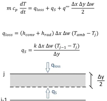
3.3.1. Internal plane

To determine the fluid temperature in an internal plane 𝑗 as schematized in Figure 3.4, an energy balance should be done maintaining energy conservation:

𝑚 𝑐_𝑝 𝑑𝑇 𝑑𝑡 = 𝑞𝑁+ 𝑞𝑆+ 𝑞’’’ ∆𝑥 ∆𝑦 ∆𝑤 (3.11) where, 𝑞𝑁 = 𝑘 ∆𝑥 ∆𝑤 (𝑇_𝑗+1− 𝑇_𝑗) ∆𝑦 (3.12) 𝑞_𝑆 =𝑘 ∆𝑥 ∆𝑤 (𝑇𝑗−1− 𝑇𝑗) ∆𝑦 (3.13)

and 𝑚 = 𝜌 ∆𝑥 ∆𝑦 ∆𝑤 is the mass of nanofluid in the volume.

Figure 3.4 – One-dimensional mesh for internal plane on a volumetric receiver

By substituting Eq. (3.12) and Eq. (3.13) into Eq. (3.11), the temperature in the node j for the instant 𝑡 + ∆𝑡 (corresponding to the supraindice k+1) is given by:

𝑇_𝑗𝑘+1 ₌𝑞𝑗′′′ 𝑘 ∆𝑡 𝜌_𝑗𝑘 _𝑐

𝑝𝑗𝑘

+ 𝐹𝑜(𝑇_𝑗+1𝑘 _{+ 𝑇}

𝑗−1𝑘 ) + 𝑇𝑗𝑘(1 − 2 𝐹𝑜) (3.14) where 𝐹𝑜 is the Fourier number that is calculated by:

𝐹𝑜 =𝛼 ∆𝑡

∆𝑦2 (3.15)

21

3.3.2. Boundary conditions

In the case of a one-dimensional mesh, the boundary conditions to restrict the model are just necessary on the top and bottom surfaces.

• Surface with convection (y=0)

Applying the heat energy balance to the top surface zone, see Figure 3.5, results the following equation: 𝑚 𝑐_𝑝 𝑑𝑇 𝑑𝑡 = 𝑞𝑙𝑜𝑠𝑠+ 𝑞𝑆+ 𝑞’’’ ∆𝑥 ∆𝑦 ∆𝑤 2 (3.16) where, 𝑞_{𝑙𝑜𝑠𝑠} = (ℎ_{𝑐𝑜𝑛𝑣}+ ℎ_𝑟𝑎𝑑) ∆𝑥 ∆𝑤 (𝑇_𝑎𝑚𝑏− 𝑇_𝑗) (3.17) 𝑞_𝑆 =𝑘 ∆𝑥 ∆𝑤 (𝑇𝑗−1− 𝑇𝑗) ∆𝑦 (3.18)

Figure 3.5 – One-dimensional mesh for top plane on a volumetric receiver

Solving energy balance equation in order to the temperature at the instant 𝑘 + 1, we obtain: 𝑇_𝑗𝑘+1 ₌𝑞𝑗′′′ 𝑘 ∆𝑡

𝜌_𝑗𝑘 _𝑐 𝑝𝑗𝑘

+ 2 𝐹𝑜(𝑇_𝑗−1𝑘 _{+ 𝐵𝑖 𝑇}

𝑎𝑚𝑏) + 𝑇𝑗𝑘(1 − 2 𝐹𝑜 − 2 𝐹𝑜 𝐵𝑖) (3.19)

where 𝐹𝑜 is the Fourier number, and 𝐵𝑖 the Biot number that is calculated by: 𝐵𝑖 =(ℎ𝑐𝑜𝑛𝑣+ ℎ𝑟𝑎𝑑) ∆𝑦

𝑘 (3.20)

The convection heat transfer coefficient depends on the air speed and receiver length (𝐿) on x direction, while the radiation heat transfer coefficient is temperature dependent [33]:

ℎ𝑐𝑜𝑛𝑣=

8,6 𝑈0,6

𝐿0,4 (3.21)

22 • Adiabatic surface (y=H)

The energy balance for a general configuration of a bottom surface as schematized according to Figure 3.6 is given by:

𝑚 𝑐𝑝 𝑑𝑇 𝑑𝑡 = 𝑞𝑁+ 𝑞𝑆+ 𝑞’’’ ∆𝑥 ∆𝑦 ∆𝑤 2 (3.23) where, 𝑞𝑁 = 𝑘 ∆𝑥 ∆𝑤 (𝑇𝑗+1− 𝑇𝑗) ∆𝑦 (3.24) 𝑞_𝑆 = (ℎ_{𝑐𝑜𝑛𝑣}+ ℎ_𝑟𝑎𝑑) ∆𝑥 ∆𝑤 (𝑇𝑎𝑚𝑏 − 𝑇𝑗) (3.25)

Figure 3.6 – One-dimensional mesh for bottom plane on a volumetric receiver

Solving Eq. (3.23) in order to the temperature at the instant 𝑘 + 1 we get: 𝑇_𝑗𝑘+1 =𝑞𝑗 ′′′ 𝑘 _∆𝑡 𝜌_𝑗𝑘 _𝑐 𝑝𝑗𝑘 + 2 𝐹𝑜(𝑇𝑗+1 𝑘 _{+ 𝐵𝑖 𝑇} 𝑎𝑚𝑏) + 𝑇𝑗𝑘(1 − 2 𝐹𝑜 − 2 𝐹𝑜 𝐵𝑖) (3.26) However, since the bottom surface of the receiver is adiabatic, Biot number equals zero, and equation (3.26) results in:

𝑇_𝑗𝑘+1= 𝑞𝑗 ′′′ 𝑘 _∆𝑡 𝜌_𝑗𝑘 _𝑐 𝑝𝑗𝑘 + 2 𝐹𝑜 𝑇𝑗+1 𝑘 _{+ 𝑇} 𝑗𝑘(1 − 2 𝐹𝑜) (3.27)

23

3.4. Receiver efficiency

For the particular case where a fluid is stationary, undergoing transient heating, and considering heat transfer on one dimension (y), the receiver’s efficiency can be calculated by the ratio of the total absorbed thermal energy to the total incident energy over a period of time:

𝜂 =

∑ 𝜌(𝑛𝑗 𝑗) 𝑐_𝑝(𝑗) (𝑇_𝑓(𝑗) − 𝑇_𝑖(𝑗)) ∆𝑦 𝑗

𝐶 𝐺 𝑡 (3.28)

where 𝜌(𝑗) and 𝑐𝑝(𝑗) are the local density and specific heat capacity of the fluid. 𝑇𝑓(𝑗) represents the local temperature at the last instant, and 𝑇𝑖 the initial temperature as function of y position. Finally, 𝑡 is the total time that the receiver is exposed to solar radiation (𝐶 𝐺).

3.5. Numerical results

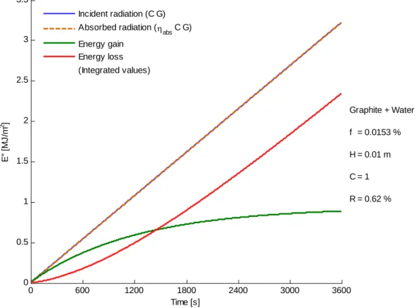
The numerical model to determine the temperature profile on a volumetric receiver described in the previous section was implemented in Matlab. The developed program allows the comparison between eight distinct nanofluids that result from the different combinations between two carbon-based nanoparticles (graphite and multi-walled carbon nanotubes) and four base fluids (pure water, Therminol VP1, Perfecto HT 5 and ethylene glycol). With such program it is also possible to insert the desired nanoparticle volume fraction (𝑓𝑣) and receiver height (H), as well as optimize one of these two variables, according to the optical properties discussed in Chapter 2.

The following outputs were obtained from simulations considering a constant input of solar radiation at the top of the receiver (y = 0). Since collimated rays were assumed, it is more adequate

to use the solar spectral distribution defined in AM1.5 Direct, where the numerical integration of Eq.

(3.2) and derivative of Eq. (3.1) are calculated using the discrete values between a wavelength range from 280 nm to 2500 nm. As to the parameters that affect heat loss, air speed was set to be 0,5 m/s, ambient temperature to 25°C, and glass emissivity to 0,95. The initial temperature of the different nanofluids was 25°C, which was also used to determine their thermodynamic properties according to the model presented in Chapter 2.

24

3.5.1. Heat release profile

• Heat release profile for fixed volume fraction and height:

As an example, the heat release profile on y direction for a 1 cm height volumetric receiver and with ∆𝑦 = 7E-5 𝑚, containing either graphite or MWCNT nanoparticles suspended on different base fluids with a volume fraction of 0,01%, is shown in Figure 3.7.

Figure 3.7 – Heat release profile (H = 0,01 m; fv = 0,01%)

The results show that heat release decreases with increasing depth. This decrease was expected, since light is attenuated as it is absorbed by the nanofluid along the path. It is also visible that the different nanofluids have a very similar variation to what concerns light extinction. Note that, if solar concentration factor increases, a similar profile is obtained but the magnitude of heat release would increase while absorption efficiency remains the same. For the previous conditions of volume fraction and receiver height, Table 3.1 presents the obtained absorption efficiencies. We conclude that solid particles have the most impact on energy absorption because higher efficiencies are attained when comparing to the ones registered for different base fluids. Results also indicate that amongst the eight nanofluids, using MWCNT suspensions with water as base fluid is more convenient because the highest absorption efficiencies are achieved.

0 2 4 6 8 10 x 105 0 0.001 0.002 0.003 0.004 0.005 0.006 0.007 0.008 0.009 0.01 q´´´ [W/m3] y [ m ] f = 0.01 % H = 0.01 m C = 1 Graphite + Water Graphite + Therminol VP1 Graphite + Perfecto HT 5 Graphite + Ethylene Glycol MWCNT + Water

MWCNT + Therminol VP1 MWCNT + Perfecto HT 5 MWCNT + Ethylene Glycol

25

Table 3.1 – Comparison between absorption efficiency for different nanofluids (H = 0,01 m; fv = 0,01%)

The numerical error associated to this methodology was also determined (see Eq. (9.2) in appendix III) and the obtained numerical residue values are shown in Table 3.2. Since the magnitude of the error depends on the calculated absorption efficiency, as a consequence, its impact will alter the temperature values of the volumetric receiver. Nonetheless, the numerical error reveals to be relatively small.

Table 3.2 – Numerical error for different nanofluids (H = 0,01 m; fv = 0,01%)

R [%] Graphite MWCNT

Water 0,1314 0,1469

Therminol VP1 0,0911 0,0484 Perfecto HT 5 0,0966 0,0521 Ethelyne glycol 0,0810 0,0695

• Heat release profile for fixed height (optimize volume fraction):

In Figure 3.8 it is shown that increasing nanoparticle’s volume fraction will result in an increase of absorption efficiency, until a point where adding nanoparticles to the base fluid will not significantly increase absorption efficiency or it will reach 100%. Therefore, an optimization of volume fraction will enable to greatly reduce a lot the quantity of nanoparticles that are needed to achieve a certain absorption efficiency for a particular receiver’s height.

𝜂𝑎𝑏𝑠[%] Graphite MWCNT

Water 99,869 99,969

Therminol VP1 99,314 99,960

Perfecto HT 5 99,322 99,965

26

Figure 3.8 – Effect of volume fraction on absorption efficiency

Note that optimum values of volume fraction are characteristic of the receiver height and the nanofluid composition, but not the magnitude of the incident flux. To numerically determine this optimum volume fraction, both receiver height and absorption efficiency were set as independent parameters so that Newton’s method (see appendix IV) could be implemented. As expected, according to the results shown in Table 3.3, MWCNT suspended in water revealed to have properties that allow better absorption, and thus, lower volume fraction is required to achieve a given absorption efficiency.

Table 3.3 – Optimum volume fraction for 99,99% absorption efficiency (H = 1 cm; Δy = 0,006 cm)

𝑓𝑣 𝑜𝑝𝑡[%] Graphite MWCNT

Water 0,015296 0,011499

Therminol VP1 0,027664 0,011817 Perfecto HT 5 0,027666 0,011629 Ethelyne glycol 0,016896 0,011596

As to the numerical error, calculated using Eq. (9.2) in appendix III, it is possible to realize that the residual of graphite nanoparticles is higher than the ones obtained with MWCNT. However, these values are always below 1%, so the impact is relatively small, as shown in Table 3.4.

0 1 2 3 x 10-4 0 10 20 30 40 50 60 70 80 90 100 Volume fraction (f v) abs (fv ) [ % ] H = 0.01 m Graphite + Therminol VP1

27

Table 3.4 – Numerical error for different nanofluids (H = 1 cm; Δy = 0,006 cm; ƞabs = 99,99%)

R [%] Graphite MWCNT

Water 0,16901 0,12471

Therminol VP1 0,54229 0,049455 Perfecto HT 5 0,55128 0,050405 Ethelyne glycol 0,1733 0,064125

The volumetric heat rate can also be represented in dimensionless form in the following way: 𝑞𝑟 =

𝑞 𝐻

𝑃(𝑦 = 0) (3.29)

where 𝑃(𝑦) is the radiative flux as function of height, see Eq. (3.2).

The impact of different heights on 𝑞𝑟, while maintaining a fixed absorption efficiency, has also been tested. From the example given in Figure 3.9 with an absorption efficiency of 99,99%, we conclude that the dimensionless heat release profile is invariant with channel height. The small difference between the results can be explained by the numerical residual error.

Figure 3.9 – Dimensionless heat release profile for different heights

0 1 2 3 4 5 6 7 8 9 10 0 0.1 0.2 0.3 0.4 0.5 0.6 0.7 0.8 0.9 1 qr y /H Graphite + Therminol VP1 C = 1 f 1 = 0.0277 % R 1 = 0.5423 % f 2 = 0.0025 % R 2 = 0.0168 % H 1 = 0.01 m H 2 = 0.1 m

28

• Heat release profile for fixed volume fraction (optimize height):

Since thermal loss was only considered through the top surface, increasing the receiver height will also increase the absorption efficiency, as shown on Figure 3.10.

Figure 3.10 – Effect of receiver height on absorption efficiency

However, to reduce as much as possible the receiver’s size without compromising efficiency and still maintaining the same volume fraction, the same numerical method used before (see appendix IV) can also be applied, in this case, to determine the ideal receiver height (H). Results lead to the same conclusions as in Table 3.3, in which the numerical residue for the eight combinations of base fluid and particles is lower than 1% in all those cases.

3.5.2. Temperature profile

As seen until now, there are a lot of variables which, either related to the receiver geometry, nanofluid properties or atmospheric conditions, can originate a significant divergence between simulated results. To try and study the mechanisms of heat transfer inside a volumetric receiver, some variables were set as constant inputs while varying others to evaluate their impacts. Hence, the following outputs were obtained from simulations using the model described in section 3.2 and in section 3.3, by considering that 99,99% of solar radiation is absorbed by each nanofluid for a fixed receiver height of 1 cm (∆𝑦 = 6E-5 𝑚) and for the optimum values of volume fraction of Table 3.3.

0 0.005 0.01 0.015 0.02 0 10 20 30 40 50 60 70 80 90 100 Height [m] ab s (H ) [% ] f = 0.01 %

29

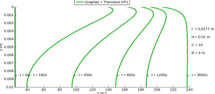
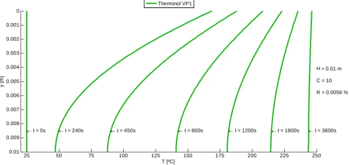
The temperature profile on a volumetric receiver is perceptible by analyzing Figure 3.11 which represents, as an example, temperature distribution on transient regime for graphite nanoparticles suspended in HTF Therminol VP1 under constant solar radiation. From these results, we can point out that before 1200 seconds (approximately), the temperature on the top surface is higher than the one on the bottom surface. However, after this instant, the temperature on the top surface becomes lower than the bottom one. This happens not only due to heat loss on the top surface, but also because the lower fluid layers keep absorbing solar radiation. Thus, conduction flux changes direction and heat transfer starts to go upwards.

Figure 3.11 – Temperature profile in transient regime for a graphite-based receiver

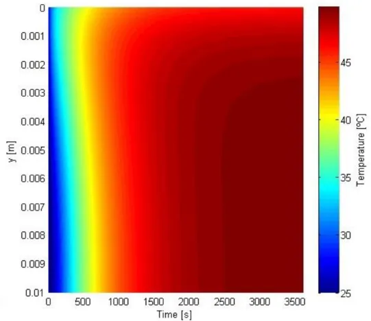
Similar profiles were obtained for the remaining nanofluids, in which another example is shown in Figure 3.12, with MWCNT suspended in Perfecto HT 5 for a lower solar concentration factor.

Figure 3.12 – Temperature profile in transient regime for a MWCNT-based receiver

40 60 80 100 120 140 160 180 200 220 240 0 0.001 0.002 0.003 0.004 0.005 0.006 0.007 0.008 0.009 0.01 T [ºC] y [ m ] f = 0.0277 % H = 0.01 m C = 10 R = 5 %  t = 0s t = 180s  t = 450s  t = 800s  t = 1200s  t = 3600s Graphite + Therminol VP1 25 30 35 40 45 50 0 0.002 0.004 0.006 0.008 0.01 T [ºC] y [ m ] f = 0.0116 % H = 0.01 m C = 1 R = 0.41 %  t = 0s  t = 180s  t = 450s  t = 800s  t = 1200s  t = 3600s MWCNT + Perfecto HT 5

30

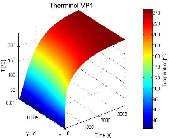
For this case, the conduction flux changes direction approximately at 800 seconds. The temperature distribution was also represented on a coloured plot:

Figure 3.13 – Coloured temperature profile in transient regime for a MWCNT-based receiver

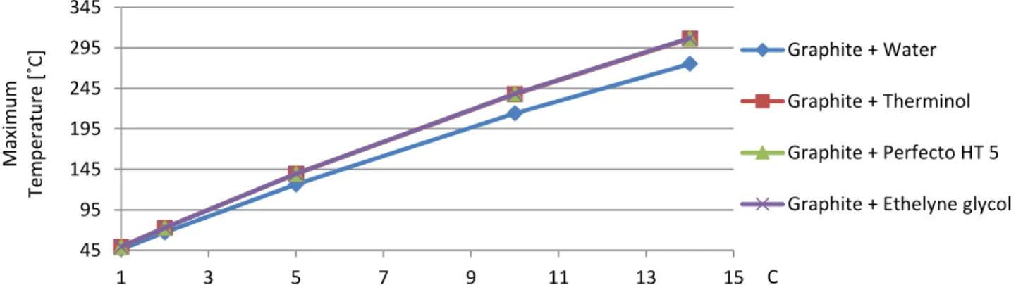
At the end of the simulated time (3600 seconds) the maximum temperatures obtained for different solar concentration factors are shown in Table 3.5.

Table 3.5 – Maximum temperature for different solar concentration factors (H = 1 cm; ƞabs = 99,99%; time = 1 hour)

Tmax [°C] C = 1 C = 2 C = 5 C = 10 C = 14

Graphite + Water 46,28 67,07 126,29 * 214,14 * 275,24 * Graphite + Therminol VP1 49,16 72,69 139,35 237,70 306,35 * Graphite + Perfecto HT 5 49,23 72,82 139,66 238,27 307,11 Graphite + Ethelyne glycol 48,28 71,00 135,55 * 231,19 * 298,06 *

MWCNT + Water 46,36 67,23 126,64 * 214,69 * 275,84 *

MWCNT + Therminol VP1 49,72 73,78 141,95 242,51 312,77 *

MWCNT + Perfecto HT 5 49,78 73,90 142,22 243,04 313,50

MWCNT + Ethelyne glycol 48,21 70,83 134,96 * 229,53 * 295,27 * * Valid when considering saturated liquid (no phase change)