A tool to manage tasks of R&D projects
Joana Fialho
∗, Pedro Godinho
†, João Paulo Costa
†∗ Escola Superior de Tecnologia e Gestão de Viseu, Instituto Politécnico de Viseu, Portugal
E-mail:jfialho@ estv. ipv. pt
† Faculdade de Economia da Universidade de Coimbra
E-mail(Pedro Godinho):pgodinho@ fe. uc. pt E-mail (João Paulo Costa):jpaulo@ fe. uc. pt
Abstract
We propose a tool for managing tasks of Research and Development (R&D) projects. We define an R&D project as a network of tasks and we assume that different amounts of resources may be allocated to a task, leading to different costs and different average execution times. The advancement of a task is stochastic, and the management may reallocate resources while the task is being performed, according to its progress. The operational cash flows depend on the task completion time, and their expected values follow a stochastic process. We consider that a strategy for completing a task is a set of rules that define the level of resources to be allocated to the task at each moment. We discuss the evaluation of strategies for completing a task, and we address the problem of finding the optimal strategy.
Key words: R&D task management and evaluation, real options, stochastic models, simulation, optimal decisions.
1
Introduction
Companies operating in dynamic markets, driven by technological innovation, need to decide, at each moment, which projects to carry out and the amount of resources to allocate to them. These decisions are crucial for the companies’ success. R&D projects are characterized by several types of uncertainty and by the possibility of changing the initial plan of action, that is, R&D projects have two very important features that have to be taken into account: uncertainty and operational flexibility. The flexibility of a project leads to an increase in the project value that must be taken into account in its analysis or evaluation. When there is operational flexibility, it may be better to change the plan of action when new information arrives.
Traditional project evaluation methods, such as the ones based on discounted cash flows, are not adequate because they assume a pre-determined and fixed plan, which does not allow taking into account both uncertainty and flexibility (Yeo and Qiu, 2003).
The recognition that the financial options theory can be used to evaluate investment projects was made by Myers (1984), who used the expression real option to express the management flexibility under un-certain environments. Real options theory allows us to determine the best sequence of decisions to make in an uncertain environment, and provides the proper way to evaluate a project when such flexibility is present. The decisions are made according to the opportunities that appear along the project life time, which means that the optimal decision-path is chosen step by step, switching paths as events and opportunities appear (Cortazar et al., 2008).
To evaluate or analyze an R&D project, it is important to evaluate the sequential real options that appear along the life time of the project. To evaluate these options, it is important to incorporate the associated risk. This risk may be related to prices, costs and technology, among others. There are several processes to model these variables, like Brownian motions (Cortazar et al., 2003), mean reversing models (Copeland and Antikarov, 2001), controlled diffusion processes (Schwartz and Zozaya-Gorostiza, 2003), or even combinations between diffusion and Poisson processes (Pennings and Sereno, 2011). The Pois-son processes are also widely used to model technological uncertainties (Pennings and Sereno, 2011) or catastrophic events that make it impossible to proceed with the project (Schwartz and Zozaya-Gorostiza, 2003). The revenues may also be uncertain, and it may be necessary to model them with stochastic processes (Schwartz and Moon, 2000).
We present a tool that can be applied to evaluate R&D projects, in order to help management make decisions concerning resource allocation. In developing the model, we were particularly concerned with the use of human resources, which are often the scarcer resources in this kind of projects. However, the model is flexible enough to handle other types of resources, like equipment or financial resources (e.g., for subcontracting some fractions of the tasks). The main condition to use the model is the ability to define a finite, discrete set of levels of resources that can be used at each instant, and to define the cost
per time unit of each level of resources.
The model behind the tool presented in this paper follows Godinho et al. (2007), who proposed a real options model for the analysis of R&D projects from the telecommunications sector. The model and procedure evaluation we present take into account that the main limitation and difficulty is the human resources allocation. Management needs a tool that helps define the best allocation, in order to maximize the project value. So, the evaluation procedure should define a financial value for the project and the correspondent strategy to execute it, that is, we present a tool that gives a set of rules defining the level of resources to allocate, in order to maximize the project financial value.
We consider that an R&D project is composed by different tasks, and to evaluate a project, we must evaluate its tasks. The tool herein presented intends to evaluate those tasks. The output of this tool helps management to allocate resources to tasks that compose an R&D project. Although the tool presented evaluates a task of an R&D project, it implies that the evaluation of the tasks that compose a project leads to a financial evaluation of the project. The connection between tasks will be detailed in future work, because it is necessary to determine how the tasks are linked to each other and how codependent they are. Notice that some tasks can have precedents, that is, some tasks can only begin when others are completed or if others had obtained certain results.
For each task, we assume that different resource levels can be allocated, which have different costs and different average execution times. The advance of the task is stochastic and the project manager can reallocate resources while the task is in progress. The progression of a task defines, at each moment, which is the best level of resources to allocate to it. The difference between the resource levels can be quantitative or qualitative, that is, the levels can be different due the number of persons or due the qualities/specialization of those persons. Different strategies are analyzed, and the objective is to find the optimal strategy to execute an R&D task.
The procedure we used is based on Least Squares Monte Carlo - LSMC - proposed by Longstaff and Schwartz (2001): it constructs regression functions to explain the payoffs for the continuation of an op-tion through the values of the state variables. A set of simulated paths of the state variables is generated. With the simulated paths, the optimal decisions are set for the last period. From these decisions, it is built, for the penultimate period, a conditional function that sets the expected value taking into account the optimal decisions of the last period. With this function, optimal decisions are defined for the penul-timate period. The process continues by backward induction until the first period is reached. The use of simulation allows integrating different state variables in an easy way. We elected the LSMC process due to the fact that decisions are taken according to future expectations. However, some adaptations were necessary, for example in the way time is handled.
This paper is structured as follows: section 2 presents and characterizes the model, section 3 describes the analysis procedure, section 4 presents some examples, and section 5 concludes.
2
Proposed model
We assume that each task is homogeneous and needs a certain number of identical work units to be completed. These work units can be seen as small parts of the task and the set of these parts composes the task. The work units can be executed by different resource levels, which lead to different average times to finish the task and different costs per time unit.
We consider, in our model, that there is uncertainty in the time it takes to complete a task, and conse-quently, in the costs, because they depend directly on the time to complete the task.
The costs are deterministic, per unit of time, and depend on the level of resources. We also assume that there may be a cost inherent to switching between different resource levels, that is, reallocating persons to different tasks or to different work units may entail a cost.
In the model herein presented, we do not model the revenues, but the cash flows resulting from the completion of the task. The expected operational cash flows resulting from the exploration of the in-vestment project follow a stochastic process and depends on the time it takes to complete each task.
Notice that a set of tasks composes a project. From now on, the present value of the cash flows resulting from the life time of each task (cash inflows and cash outflows) is denominated as task worth. These cash flows represent a portion of the total cash flows of the entire project. The concept of instantaneous task worth is used, which represents the present value of the task worth, assuming that the task was already finished. We also assume a penalty in the task worth according to its completion time, that is, the task worth is more penalized as the task takes longer to be completed. We admitted this penalty, because we assume that R&D projects can turn more profitable if a product or a service is launched earlier. Before the presentation of the evaluation procedure, it is necessary to introduce the modelling of the state variables. Thus, the next subsections describe in detail how we handle the time to complete a task, the task worth, the costs and the net present value of the task.
2.1
Time to complete a task
The time to complete a task is not deterministic because it is impossible to know it with certainty, due to unpredictable delays or technical difficulties. Considering a specific level of resources k along the entire task, we define the time to finish the task as T(k). T(k) is a random variable and it is a sum of
a deterministic term, the minimum time to finish the task, M(k), with a stochastic one. Let D be the
necessary number of work units to complete the task. The time it takes to complete each work unit is composed by a constant part and a stochastic one, the latter being defined by an exponential distribution. This distribution is adequate because we assume that the average number of work units completed per unit of time is constant and there is no a priori expectation as to the nature of the distribution (Folta and Miller, 2002). We also assume that the time it takes to complete one work unit is independent of the time it takes to complete the other work units. This assumption comes from the fact the work units are well defined, separated and each one starts when the previous ends. Thus, it is immediate that the necessary time, T(k), to complete the task, using the level of resources k, is defined by
T(k)= D ∑ i=1 bt(k) i (1)
where bt(k)i is the time that each work unit takes, considering the level of resources k. Each term bt(k)i can be written as bt(k) i = M(k) D + t (k) i (2)
where t(k)i follows an exponential distribution with average 1/µ(k). Replacing bt(k)
i in (1) T(k)= M(k)+ D ∑ i=1 t(k)i (3)
The time to finish the task is composed by a sum of a deterministic term, which represents the minimum time that is necessary to finish the task, with a stochastic one. This latter term is defined as the sum of
D independent and identically distributed exponential variables.
2.2
The costs
The costs are deterministic per unit of time, and depend on the level of resources and on the necessary time to complete the task. We assume that, for each level of resources, the costs increase at a constant rate, possibly the inflation rate. Considering a specific level of resources k, let Cx(k) be the instantaneous
cost, at instant x. The model for the costs can be defined by
dCx(k)= ρC
(k)
x dx (4)
where ρ is the constant rate of growth of the costs. Thus, the value of Cx(k)is
Cx(k)= C0(k)eρx (5)
where C0(k) is a constant dependent of the level of resources. The cost, C(k)j , of a work unit j that uses the level of resources k, and that begins on instant xj and ends on instant xj+1is
C(k)j = ∫ xj+1 xj Cx(k)dx = ∫ xj+1 xj C0(k)eρxdx = [ 1 ρC (k) 0 e ρx ]xj+1 xj = C (k) 0 ρ (e ρxj+1− eρxj) (6)
The present value of the cost of the work unit j with respect to an instant x0 with discount rate r is
b Cj,x(k) 0 and it is given by b Cj,x(k) 0 = ∫ xj+1 xj Cx(k)e−r(x−x0)dx = C (k) 0 erx0 ρ− r ( e(ρ−r)xj+1− e(ρ−r)xj ) (7) The expression for bCj,x(k)
0, given in (7), is valid when ρ̸= r. In the case ρ = r,
b Cj,x(k) 0= ∫ xj+1 xj Cx(k)e−r(x−x0)dx = C(k) 0 e rx0(x j+1− xj) (8)
We also assume that costs related to changes of the level of resources can occur. That is, if there is a change in the level of resources from one work unit to another, it may be necessary to incur a cost. The cost for changing the level of resources from kj in the work unit j to other level of resources, kj+1, in the
next work unit j + 1 is given by γ(kj, kj+1). We also assume that these costs are deterministic, depend
on the level of resources and grow with the same rate ρ. If the change occurs at moment xj+1, that is,
at the moment that work unit j + 1 begins, the value of the respective cost is γ(kj, kj+1)eρxj+1 and the
present value of this cost, with respect to an instant x0 is
γ(kj, kj+1)eρxj+1e−r(xj+1−x0)
In our evaluation procedure, it is necessary to calculate the present value of the total remaining costs, that is, it is necessary to determine the total costs from a certain work unit j until the last one, D. We assume that, for all work units, j = 1, ..., D, the present value of the remaining costs are determined with respect to xj, which is the instant in which the work unit j starts, and it is denoted as T otC(j, xj). The
expression of T otC(j, xj) can be given by
T otC(j, xj) = D∑−1 a=j [ b C(ka) a,xj + γ(ka, ka+1)e ρxa+1e−r(xa+1−xj) ] + bC(kD) D,xj (9) where
• xj is the instant in which work unit j starts;
• bC(ka)
a,xj is the present value of the cost of the work unit a, relatively to the instant xj. The work unit
a begins at instant xa and uses the level of resources ka;
• bC(kD)
D,xj is the present value of the cost of the work unit D with respect to instant xj. The work unit
D uses the level of resources kD;
• γ(ka, ka+1) defines the value of the cost to change from the level of resources ka used in work unit
a to the level of resources ka+1used in work unit a + 1. Notice that if the level of resources is the
same in the work unit a and in the work unit a + 1, this cost is zero;
• r is the discount rate.
2.3
The task worth
We define the task worth as the present value of the cash flows resulting from completing the task (including both cash inflows and cash outflows). Thus, the task worth does not depend on the level of resources used to undertake the task, but on the time to complete it. We also define the related concept of instantaneous task worth (or instantaneous worth), which is the value of the task worth assuming that the task is completed at the instant being considered.
We assume that the instantaneous task worth changes according to a pre-defined rate and with some stochastic events. The rate can be positive or negative, depending on the nature of the project. In R&D projects, new information can arrive, or unexpected events can occur, that change the course of the project and, consequently, the expectations regarding to the instantaneous task worth. We also assume that a penalty in the instantaneous task worth may occur, due to the duration of the task. That is, we
assume that it may be the case that the earlier the product is launched in the market, the bigger is the worth obtained. The task worth may be more penalized as the task takes longer to complete. The reason for such penalty may be related to the existence of competition: if a competitor is able to introduce, earlier, a similar product in the market, the task worth might be lower.
Let the model of instantaneous worth, R, be defined by:
R dR = αR dx + R dq (10)
The parameter α included in the model represents the increasing or decreasing rate of the instantaneous worth, in each lapse dx The term dq represents a Jump process, that is
dq =
{
u, with probability pdx
0, with probability 1− pdx (11)
with u defined by a uniform distribution, u∼ U(umin, umax), umin≤ umax.
Notice that, if the instantaneous worth would depend only on the rate α, it would be continuous and monotone increasing (assuming the rate positive). But, besides the rate α, there is the possibility of occur-ring jumps in the instantaneous worth, due the nature of these projects and/or the behavior of the market. In order to handle the model, we assume the discrete version of the instantaneous worth. Ignoring the jump process, the solution of equation (10) would be Rx = R0eαx, and therefore we would have
Rx+1− Rx= R0eαx(eα− 1). Considering low values for α, we can assume α ≈ eα− 1, and the expression
would become Rx+1− Rx= αRx. In order to incorporate the jump process, we assume that in a lapse of
time that is not infinitesimal, more than one jump may take place. So, the discrete version of the model of instantaneous worth becomes
Rx+1= Rx+ αRx+ Rx∆q (12)
where ∆q =
ν
∑
i=1
ui, with ui ∼ U(umin, umax) and ν is defined by a Poisson distribution with parameter
p, that is ν ∼ P (p).
The present value of the instantaneous worth in a given moment depends on the instantaneous worth of the previous moment. Thus, the instantaneous worth of the first period is R1 = R0+ αR0+ R0∆q.
It is necessary to know the initial value R0, which is an input parameter for the model. Assuming that
the task is finished at the moment T , we define RT as the task worth calculated according to the model
previously presented.
The penalty mentioned initially can be expressed by a function g(x), where x denotes the time. This function is positive, decreasing, and it takes values from the interval [0, 1]. Thus, assuming this feature, the final expected task worth is RT× g(T ). Notice that, if there is no penalty, g(x) = 1, ∀x.
2.4
The net present value of the task
For the model, it is necessary to calculate the expected value of the net present value of the task, for each work unit j, j = 1, ..., D, and with respect to the initial instant of that work unit, xj. The net present
value of the task in each work unit includes the present value of the expected task worth at the end of the task and the present value of the total remaining costs. These present values are calculated with respect to the instant xj. Thus, assuming that the instant to finalize the task is T , the net present value of the
task, at the beginning of the work unit j is V al(j, xj), and it is determined as follows:
V al(j, xj) = RT × g(T ) × e−r(T −xj)− T otC(j, xj) (13)
3
Procedure for the task evaluation
This procedure uses a method similar to the Least Square Monte Carlo (Longstaff and Schwartz, 2001). In the beginning of the process, we build many paths with different strategies. A strategy is a set of rules that defines the level of resources to use in each work unit, possibly taking into account the way the task is progressing. The strategies used to build the paths include executing all work units with the same level of resources or using different resource levels to finish the task. For each strategy, and for each
path, we simulated the values of the time to execute the task, through the model we presented in the previous section. With the time and the level of resources used, we can determine the costs using the model presented in section 2.2, and through the model for the task worth, we can simulate the values for the instantaneous worth; finally, we can determine the net present value of the task, for each path, and for each work unit.
In this procedure we build, by backward induction and for all work units, regression functions for values previously calculated for the paths. These functions explain the net present value of the task in order to different state variables which are the elapsed time, the instantaneous worth and the number of work units already finished.
The evaluation procedure begins in the last work unit. For all paths initially simulated, it is considered the instantaneous worth observed in the beginning of the last work unit, as well as the time elapsed until the start of that work unit. For all paths, assuming a specific level of resources, kD, to complete the last
work unit, the time to complete the task is redefined, as well as the net present value of the task in the beginning of the last work unit. Taking the net present value of the task recalculated in all paths, V|kD,
the elapsed time until the beginning of the last work unit, Y1,D, and the instantaneous worth observed
in the beginning of the last unit, Y2,D, a regression function, FD,kD, is built. This function explains the
net present value of the task, in the last unit, as function of the elapsed time until the beginning of the last work unit and of the instantaneous worth observed in the beginning of that unit. We regress V|kD
on a constant, Y1,D, Y2,D, Y1,D2 , Y 2
2,D and Y1,DY2,D, that is,
FD,kD = a0+ a1Y1,D+ a2Y2,D+ a3Y1,DY2,D+ a4Y
2
1,D+ a5Y2,D2
We assumed these basis functions for the regression, but other basis functions could be selected without interfering or altering the process (Stentoft, 2004).
This procedure is repeated assuming the other resource levels to perform the last work unit. Thus, consid-ering that there are N resource levels, in the last work unit, for each level of resources kD, kD= 1, ..., N ,
we define a function, FD,kD, which explains the net present value of the task as function of the elapsed
time (until the beginning of the last unit) and of the instantaneous worth observed in the beginning of that unit.
For the earlier work units, the procedure is based on the same principle: it is considered that the work unit under consideration, say j, is executed with a specific level of resources, kj. Next, the net present
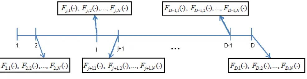
value of the task in the beginning of that unit is recalculated, through the definition of the best strategy from the following unit until the last one. The definition of the best strategy is done using the regression functions already determined (Figure 1) and the costs for switching levels: for each of the following work units, the level of resources chosen is the one that leads to a higher value in the difference between the respective regression function and the cost of switching the level (if the level of resources is different from the level used in to the previous work unit), that is, for a = j + 1, ..., D, the level of resources chosen ka
is
max
ka=1,...,N
{Fa,ka− γ(ka−1, ka)e
ρxa}
Figure 1: Functions that allow the definition of the best strategy from unit j + 1 until the last unit D.
Assuming the specific level of resources used in the unit j, and with the best strategy defined from the work unit j + 1 until the last one, we recalculate the net present value of the task in the beginning of the unit j. Taking the recalculated values of the net present value of the task, V|kj, the values of the
elapsed time until the beginning of the unit j, Y1,j and the values of the instantaneous worth observed
in the same moment, Y2,j, a regression function is defined. This regression function explains the net
present value of the task as a function of the elapsed time until the beginning of work unit j and of the instantaneous worth observed in the beginning of work unit j.
For this work unit j the procedure is repeated, assuming the other resource levels to execute it. In this way, we construct regression functions for all resource levels in the work unit j. These functions explain the net present value of the task as a function of the elapsed time and of the instantaneous worth. The process proceeds by backward induction until the second work unit. This procedure allows having, for each work unit and for all resource levels, a regression function that estimates the net present value of the task, through the elapsed time and through the instantaneous worth observed (Figure 2).
Figure 2: Regression functions, explaining the task value as function of elapsed time and instantaneous task worth.
For the first unit we do not construct the regression functions, due the fact of, for all paths, the instan-taneous worth observed in the beginning of the first unit is R0 and the elapsed time in that moment is
0, that is, the instantaneous worth observed and the elapsed time are constant. Thus, to evaluate the best strategy in the first work unit, a specific level of resources is assumed. Then, with the regression functions of the following work units, the best strategy is defined for all paths. With the best strategy in each path, the net present value of the task is calculated for the first work unit. The average of these values provides the task value, assuming that specific level of resources for the first unit. This evaluation is repeated, assuming the other resource levels for the first work unit. Notice that it is necessary to decide which level of resources may be used to begin the task. The level leading to a bigger average value of the task in the first unit, is chosen to initialize the task. After this procedure, the regression functions allow defining rules which can guide management in the decisions about the strategy to use. Thus, with the regression functions and knowing which level of resources was used, we can define rules, indicating management which is the level of resources to use next.
4
Numerical results
To test the evaluation procedure, we consider a project that is being executed. One of its tasks needs to be evaluated in order to be initialized. There are two different resource levels (level 1 and level 2) to execute the task and management needs to know which one will be used in the beginning of the task. For this specific task, D = 20 work units were defined, that is, the task is divided in 20 identical parts. We assume that, in average, level 1 can conclude 1.5 work units per unit of time, and level 2 can conclude 3 work units per unit of time. The costs increase at a rate of 0.5% per unit of time, and the discount rate is
r = 0.1%, per unit of time. We assume that the instantaneous task worth increases 1% per unit of time.
The penalty function for the instantaneous worth punishes it up to 10%, if the task takes less than 10 units of time; if the task takes between 10 and 15 units of time, the task worth is penalized up to 30%; if the task takes longer than 15 units of time, the penalty is fixed: 30%. Thus, the penalty function, g(x), where x represents time, is the following:
g(x) = 1−10x × 0.1, se x≤ 10 0.9−15x−10−10 × 0.2, se 10 < x ≤ 15 0.7, se x > 15
Table 1: Input parameters for the numerical results.
Time M(1)= M(2)= 0; µ(1)= 1.5; µ(2)= 3
Costs C0(1)= 10; C0(2)= 40; γ(kj, kj+1) = C kj+1
0 ; ρ = 0.5%
Task worth R0= 2000; α = 1%; ν∼ P (0.4); ui ∼ U(−0.2, 0.2)
To run the evaluation procedure, 700 paths were considered and we used the following initial strategies: to execute the whole task with the first level of resources; to execute the whole task with the second level of resources; to execute half of the task with one level and the other half with the other level of resources. This led to a total of 2100 paths. The paths built, using only the level 1, led to an average time of 13.28, with a net present value of 1637.6. The paths built, using only the level 2, led to an average time of 6.64, with a net present value of 1708.5.
After running the procedure described in the previous section, the average time to execute the task is 8.4 and the net present value of the task is 1728.58.
Analyzing the results of the strategy used, level 2 is the only one chosen in the first units, but afterwards level 1 is chosen in many paths (Figure 3).
In order to analyze the procedure, we can assay which one is the indicated level of resources for the next work unit. If we know the level of resources used before and the regression functions of the next work unit, it is possible to choose the level of resources that should execute the next work unit, taking into account the state variables information. The best decisions can be plotted as regions in the two-dimension space defined by the instantaneous worth and by the elapsed time. Such plot can provide some intuition about the best choices concerning the level of resources to be used in the next work unit. If in a certain work unit d, level 1 was used, the equation to determine the frontier lines between "continuing with level 1" and "change to level 2" regions are defined by Fd+1,1(·) = Fd+1,2(·) − γ(1, 2)eρxd+1. Similarly, if in a certain
work unit d, level 2 was used, the equation to determine the frontier lines between the "continuing" and "change" regions is Fd+1,1(·) − γ(2, 1)eρxd+1 = Fd+1,2(·).
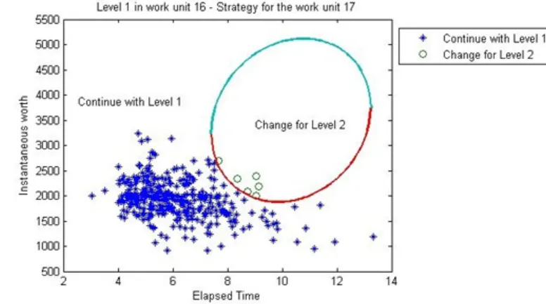
For example, assume that unit 16 of the task is completed. Supposing that level 1 was used in unit 16, we can provide a plot that defines how the level of resources should be chosen for work unit 17. This plot defines two regions, "continue with level 1" and "change to level 2", with the frontier lines obtained through F17,1(·) = F17,2(·) − γ(1, 2)eρx17. Besides these frontier lines, we also plotted choice of paths for
work unit 17, when level 1 was used in work unit 16 (Figure 4). The little stars in Figure 4 correspond to the paths that used level 1 in unit 16 and continue with level 1 in unit 17. The little balls correspond to the paths that used level 1 in work unit 16 and changed to level 2 in work unit 17. According to the region in which the pair (elapsed time, instantaneous worth) is situated, it is possible to define the level of resources to use in unit 17.
Figure 3: Percentage of the paths that choose each level of resources, after applying the evaluation process.
Figure 4: Strategy for work unit 17, when level 1 is used in the unit 16.
Now, we analyze the changes in the net present value of the task, when some parameters of the model are altered. To perform this analysis, we consider the example given above. The net present value in the
beginning of the task can be different, depending on whether or not there are costs for switching the level of resources, and depending whether or on there is a penalty in the task worth. The Table 2 contains the net present value of the task for each case.
Table 2: Net present value of the task considering the existence or not of penalty in the task worth and/or costs to switch level.
Costs to switch level Penalty Net present value of the task in its beginning
Yes Yes 1728.6
No Yes 1733.0
No No 2097.3
Yes No 2097.7
The most significant increase in the net present value of the task occurs when we remove the task worth penalty. The removal of the cost of switching level might not change the net present value of the task very much, but changes the strategy to use. Notice that the inexistence of these costs leads to more changes of level, like shown in Figure 5. Notice that this happens if there is not a dominant level, that is, if there is not a level that leads to a higher net present value of the task in all work units.
Figure 5: Percentage of the paths that choose each level of resources, after applying the evaluation process without costs to switch level of resources.
5
Concluding remarks
This work presents a tool for managing tasks of R&D projects, defining the strategy to execute a task which will lead to a higher net present value. This strategy consists in defining the level of resources to use, at each instant.
This approach can be improved by introducing an abandonment option, when the expected net present value is equal to or lower than a certain reference value. This option must be integrated and interpreted in the context of the project that contains the task.
Considering that an R&D project is a set of tasks, this evaluation procedure can be the basis to analyze the strategy to execute an R&D project, as well as the financial value associated. However, there are some aspects that must be taken into account: the result of the evaluation of a task influences the evaluation of the next task. On the other hand, the connections between the tasks and the way these connections influence the evaluation of an R&D project must also be taken into account.
References
[1] [Copeland and Antikarov, 2001] Copeland, T. and Antikarov, V. (2001). Real Options. Texere, New York.
[2] [Cortazar et al., 2008] Cortazar, G., Gravet, M. and Casassus, J. (2008). The valuation of mul-tidimensional American real options using the LSM simulation method. Computers & Operations
Research, 35: 113-129.
[3] [Cortazar et al., 2003] Cortazar, G., Schwartz, E. and Casassus, J. (2003). Optimal exploration in-vestments under price and geological-technical uncertainty: a real options model. R&D Management, 31(2): 181-189.
[4] [Folta and Miller, 2002] Folta, T. B. and Miller, K. D. (2002). Real options in equity partnerships.
Strategic Management Journal, 23(1): 77-88.
[5] [Godinho et al., 2007] Godinho, P., Regalado, J. and Afonso, R. (2007). A Model for the Application of Real Options Analysis to R&D Projects in the Telecommunications Sector. Global Business And
Economics Anthology II, 34: 63-76.
[6] [Longstaff and Schwartz, 2001] Longstaff, F. and Schwartz, E. (2001). Valuing American Options by Simulation: A Simple Least-Square Approach. The Review of Financial Studies, 14: 1113-1147. [7] [Myers, 1984] Myers, S. C. (1984). Finance theory and finance strategy. Interfaces, 14(1): 126-137. [8] [Pennings and Sereno, 2011] Pennings, E. and Sereno, L. (2011). Evaluating pharmaceutical R&D
under technical and economic uncertainty. European Journal of Operational Research, 212: 374-385. [9] [Rodrigues and Armada, 2006] Rodrigues, A. and Armada, M. (2006). The Valuation of Real Options with the Least Squares Monte Carlo Simulation Method. Management Research Unit, University of
Minho, Portugal, Available at http://ssrn.com/abstract=887953 (last access in 18-02-2013)
[10] [Schwartz and Moon, 2000] Schwartz, E. and Moon, M. (2000). Rational Pricing of Internet Com-panies. Financial Analysts Journal, 56(3): 62-75.
[11] [Schwartz and Zozaya-Gorostiza, 2003] Schwartz, E. and Zozaya-Gorostiza, C. (2003). Investment Under Uncertainty in Information Technology: Acquisition and Development Projects. Management
Science, 49(1): 57-70.
[12] [Stentoft, 2004] Stentoft, L. (2004). Convergence of the Least Squares Monte Carlo Approach to American Option Valuation. Management Science, 80(9): 1193-1203.
[13] [Yeo and Qiu, 2003] Yeo, K. T. and Qiu, F. (2003). The value of management flexibility - a real option approach to investment evaluation. International Journal of Project Management, 21: 243-250.