Deep Learning for Market Forecasts

FACULDADE DE

ENGENHARIA DA

UNIVERSIDADE DO

PORTO

Deep Learning for Market Forecasts

Gonçalo Duarte Lima Freire Lopes

Mestrado Integrado em Engenharia Informática e Computação Supervisor: Eugénio Oliveira

Deep Learning for Market Forecasts

Gonçalo Duarte Lima Freire Lopes

Abstract

Behavioral Finance combines psychology and finance in order to predict and justify why people make irrational financial decisions. With the increasing growth of social interaction on the internet, it becomes possible to use Opinion Mining techniques to extract social trends and investor sen-timent about specific assets. Previous literature has proven the correlation between stock market prices and online sentiment.

The process of opinion mining is defined as identifying opinions in pieces of text and labeling them as negative, neutral or positive. Firstly, Opinion Mining was performed with lexicon based approaches. Results from these approaches were first improved with classical machine learning, using bag of words representations and support vector machines and neural networks. Recently, as with many other fields, deep learning approaches are outperforming other approaches but being more computationally heavy.

Besides using opinion mining to predict price movements, regression techniques are also an option for prediction, taking only price data into account. As with opinion mining, regression techniques have become more accurate in recent years with the usage of deep learning approaches. Although both opinion mining and regression have proven themselves accurate for market price predictions, few work has been published which integrates both opinion mining and regres-sion to construct a more powerful price prediction model. The goal for this work is to construct such a model, using deep learning approaches. More specifically, the constructed model will aim to predict price fluctuations in cryptocurrency markets. These markets are highly volatile and very influenced by social trends and sentiment. Also, publications about cryptocurrency markets are still short in number.

To achieve this goal, an opinion mining system will first be built, to extract opinion values for different currencies, utilizing different opinion mining models. Afterwards, combining the result of the opinion mining system and real time price data, multiple models which combine both inputs will be built, so their accuracies may be compared.

Given successful experiments in model building, this will emphasize the importance of us-ing both behavioral finance and financial methods to perform price predictions. Besides this, an opinion mining system and a price prediction model will be built for cryptocurrency markets.

Acknowledgements

I would like to thank Prof. Eugénio Oliveira and Prof. Virginia Dignum for helping me with research and writing decisions and providing guidance and motivation.

I also want to express my gratitude to my parents for raising me with drive and desire to continuously better myself and achieve more.

Finally, I’d like to thank Roddy for motivating me to study financial markets and economics.

Thank you

‘I can calculate the motion of heavenly bodies, but not the madness of people.‘

Contents

1.1.4 Blockchain and Cryptocurrencies . . . 3

1.2 Motivation . . . 4

1.3 Goals . . . 5

1.4 Structure of the Report . . . 5

2 State of the Art 7 2.1 Opinion Mining . . . 7 2.1.1 Preprocessing . . . 7 2.1.2 Representations . . . 8 2.1.3 Methodologies . . . 9 2.1.4 Datasets . . . 11 2.1.5 Related Work . . . 11 2.2 Price Prediction . . . 12 2.2.1 Financial Methods . . . 12 2.2.2 Machine Learning . . . 12 2.2.3 Deep Learning . . . 12 2.2.4 Datasets . . . 13 2.2.5 Related Work . . . 13 3 Conceptual Model 15 3.1 Architecture . . . 15 3.2 Cryptocurrencies . . . 16 3.3 Data Sources . . . 16 3.3.1 Price Data . . . 16 3.3.2 Opinion Mining . . . 16 3.4 Preprocessing . . . 17 3.4.1 Timeframes . . . 17 3.4.2 StockTwits . . . 17 3.5 Algorithms . . . 17 3.5.1 Opinion Mining . . . 17 3.5.2 Price Prediction . . . 20 3.6 Benchmarking . . . 22 3.6.1 Opinion Model . . . 22

CONTENTS 3.6.2 Price Prediction . . . 22 4 Implementation 27 4.1 Data Collection . . . 27 4.1.1 Opinion Mining . . . 27 4.1.2 Price Prediction . . . 27 4.2 Preprocessing . . . 27 4.2.1 Opinion Mining . . . 27 4.2.2 Price Prediction . . . 28 4.3 Training . . . 28 4.3.1 Opinion Mining . . . 28 4.3.2 Price Prediction . . . 31 5 Results 35 5.1 Opinion Mining . . . 35 5.1.1 CNN . . . 35 5.1.2 LSTM . . . 35 5.1.3 Conclusion . . . 36 5.2 Price Prediction . . . 36 5.2.1 Mechanical Strategies . . . 36 5.2.2 No opinion data . . . 37 5.2.3 Opinion data . . . 38 6 Conclusions 41 6.1 Future Work . . . 42 6.2 Self-reflection . . . 42 References 45 viii

List of Figures

3.1 Architecture . . . 15

3.2 Simplified architecture of the CNN used. Figure is taken from Cliche [Cli17] . . 18

3.3 Simplified architecture of the LSTM used. Figure is taken from Cliche [Cli17] . . 19

3.4 Japanese Candlestick. Figure is taken from [inv18a] . . . 20

3.5 SFM architecture. Figure is taken from [ZAQ17] . . . 21

3.6 Moving Average Crossover Strategy. Figure is taken from [the18] . . . 22

3.7 MACD Crossover Strategy. Figure is taken from [onl18] . . . 23

3.8 RSI Overbought Oversold Strategy. Figure is taken from [mql18] . . . 24

LIST OF FIGURES

List of Tables

5.1 CNN Opinion Model - MSE (dropout/regularizer) . . . 35

5.2 LSTM Opinion Model - MSE (dropout/units/regularizer) . . . 35

5.3 1 day timeframe %-ROI . . . 36

5.4 4 hour timeframe %-ROI . . . 36

5.5 30 minute timeframe %-ROI . . . 37

5.6 1 day LSTM(units/dropout/regularizer) . . . 37 5.7 4 hour LSTM(units/dropout/regularizer) . . . 37 5.8 30 minute LSTM(units/dropout/regularizer) . . . 37 5.9 1 day SFM(dropout/regularizer) . . . 38 5.10 4 hour SFM(dropout/regularizer) . . . 38 5.11 30 minute SFM(dropout/regularizer) . . . 38 5.12 1 day LSTM Opinion(units/dropout/regularizer/embedding/opinion) . . . 38 5.13 4 hour LSTM Opinion(units/dropout/regularizer/embedding/opinion) . . . 39 5.14 30 minute LSTM Opinion(units/dropout/regularizer/embedding/opinion) . . . 39 5.15 1 day SFM Opinion(dropout/regularizer/embedding/opinion) . . . 39 5.16 4 hour SFM Opinion(dropout/regularizer/embedding/opinion) . . . 40 5.17 30 minute SFM Opinion(dropout/regularizer/embedding/opinion) . . . 40

5.18 Best obtained model - SFM opinion data . . . 40

Chapter 1

Introduction

1.1

Context

1.1.1 Behavioral Finance

The efficient markets hypothesis (EMH) [Fam70], assumes that, in an efficient market, all shares trade at fair values, because prices incorporate and reflect all available relevant information, leav-ing no room for investor sentiment. "Behavioral finance, in contrast, studies how people fall short of this ideal in their decisions and how markets are, to some degree, inefficient" [Hir15].

Behavioral finance aims to combine psychological and behavioral theory with finance and economics in order to explain why people make irrational financial decisions. Early studies and the formulation of the prospect theory [KT79] revealed that people are generally risk averse, and losses have a higher psychological impact than gains. This study also revealed there’s an inclination to take sure gains, rather than risking for more while the contrary occurs for losses, there’s an inclination to take risks when there’s a possibility to reduce loss. This risk aversion provides a reasonable explanation for big market crashes, which are mostly driven by investor panic at a point of sentiment reversal. Findings by [Stu14] also indicate that turning points capture investors’ collective sentiment.

Generally, we are affected by our mood when making purchase and investment decisions. [DRMN94] studied the relation between store atmosphere and purchasing behavior and findings confirm that "pleasantness experienced within a retail store environment can have a significant in-fluence on purchase". This is also true to the stock markets. [SC15b] showed that "asset prices and sentiment effects correlate positively with investor sentiment". [Ode98] concluded that investor overconfidence leads to higher trading aggressiveness and overpricing, and [BO00] showed that individual investors tend to develop their own investing strategies rather than indexing in hopes of outperforming the market, although many turn out to not only underperform the market but also generate losses rather than profit.

[De 00] showed how underreaction and overreaction lead to large upswings and downswings on the markets and that "markets are composed of imperfectly rational players in imperfect mar-kets". Overreaction is analyzed by [HR01] on an enormous surge of EntreMed stock price. "A

Introduction

Sunday New York Times article on a potential development of new cancer-curing drugs caused EntreMed’s stock price to rise from 12.063 at the Friday close, to open at 85 and close near 52 on Monday. It closed above 30 in the three following weeks. The enthusiasm spilled over to other biotechnology stocks. The potential breakthrough in cancer research already had been reported, however, in the journal Nature, and in various popular newspapers including the Times! more than five months earlier. Thus, enthusiastic public attention induced a permanent rise in share prices, even though no genuinely new information had been presented.".

This overreaction to the price of EntreMed also demonstrates availability bias, which states that "investors overweight information that is easily accessible, e.g., that is easily recalled from memory or that corresponds to a future scenario that is easy to imagine".[DSMS08]

Besides the individual behavior and psychology influence on purchasing decisions, we are also very social beings which leads to interaction with others having an influence in our beliefs and emotions. [Nof05] notes that collectively shared opinions and beliefs shape individual decisions, which aggregate into social trends. [Dwy07] measured how electronic word of mouth, activity on message boards and chat rooms influences consumer purchasing decisions.

As social media keeps its exponential growth there’s the possibility of using websites like Twitter and StockTwits, to process textual sentiment with the goal of measuring investor sentiment and making predictions on the directions of markets.

1.1.2 Opinion Mining

[KL14] reviews the research that has been done integrating textual sentiments and online message boards. Machine learning systems have been devised to classify pieces of text into buy (bullish), hold (neutral) and sell (bearish) signals.

Among the existing research, [AF04] has demonstrated that high online board activity is a predictor of price volatility while [Eng08] successfully implemented a strategy which longs stocks with articles containing no negative words and shorts the ones with articles containing more than 5% negative words.

Sentiment processing is performed with opinion mining or opinion mining techniques. opinion mining is the process of automatically identifying opinions expressed in pieces of text, labeling them as Negative, Neutral or Positive. This kind of processing may use Lexicon based approaches, machine learning based approaches or hybrid approaches. Within the field of machine learning, recent developments in deep learning have allowed opinion mining to become increasingly pow-erful, providing more accurate results every year and allowing companies to use opinion mining to aid their decision making.

As previously mentioned, Twitter has a great potential to be used for opinion mining and [BMZ10] has shown the correlation between sentiment on Twitter and the Dow Jones Industrial Average (DJIA). [NH15] has used a Twitter sentiment strategy growing a portfolio by 20% be-tween June 1 - November 31, 2013. During this time the S&P 500 index grew by 10%, which demonstrates the benefits of analyzing investor sentiment.

Introduction

More recently, [Bra17] has used exclusively president Trump’s tweets to devise a sentiment trading bot, which after 2 months of testing with a virtual portfolio, generated a return of 7%.

1.1.3 Algorithmic Trading

Traditionally, algorithmic trading was mostly exclusive to high frequency trading, which takes advantage of spreads and arbitrage opportunities to generate small profits [CL16], with traders paying millions of dollars to reduce latency by few milliseconds [O’H15].

Currently, with advances in machine learning, and more specifically, deep learning, and the use of Recurrent Neural Networks (RNN), usually based on the Artificial Neural Network (ANN) paradigm, which have reported great results at analyzing time series data, a new type of algo-rithmic trading arises, where Artificial Intelligence algorithms can use deep learning models to predict price movements. [HLS+16] and [AAA14] confirmed that machine learning approaches like Support Vector Machines (SVM) and ANN, have the potential to provide better results than regular econometric models while [LKL14] mentions the potential that recurrent neural networks have for time-series modeling.

[Per16] has used Long Short-Term Memory (LSTM) Networks with a market vector repre-sentation, and [CHP17] has used Deep Neural Networks (DNN) as deep learning approaches to predict market price. [ZAQ17] introduced a new type of deep learning model, State Frequency Memory (SFM) recurrent network, which achieved better results than the previous state of the art models.

1.1.4 Blockchain and Cryptocurrencies

After the market collapse of 2008, a person or group of people identified as a Japanese program-mer called Satoshi Nakamoto released the white paper "Bitcoin: A Peer-to-Peer Electronic Cash System" [Nak08] as a revolutionary idea to replace common fiat currency with cryptocurrency, solving issues such as fraud, inflation and slow and costly transactions.

Bitcoin transactions are recorded on the blockchain. blockchains are distributed ledgers which allow permanent record of transactions. This is what allows payments to be faster, cheaper and more secure while also removing the existence of a centralized point of failure or controlling entity. Manipulation and fraud is also near impossible as transaction records are spread throughout the decentralized network. The inner works of how blockchain technology works is beyond the scope of this thesis.

Bitcoin is obtained through Bitcoin mining, by solving a cryptographic puzzle. The first Bit-coin was mined by Satoshi Nakamoto in January 2009 [Bit14].

Bitcoin is scarce like gold and silver, with a total supply of 21 million [NMF+16], making it deflationary. This lead to Bitcoin now being used as a store of value, especially given its incredible run up in 2017, climbing from below 1000$ to a peak of 20 000$. This latest run up earned it a lot of media coverage. Past publications have called it a "dysfunctional speculation vehicle" [Han13]

Introduction

while others give it credit for its use for e-commerce and medium of exchange but critique its potential as a store of value given its very high volatility [GI13].

Many teams of developers are now using blockchain technology to develop other ecosystems and cryptocurrencies each with its own use cases. As of January 2018, there are over 1400 different cryptocurrencies [Coi18b]. Most of these cryptocurrencies are available for trading in exchanges, just like stocks with a difference being the fact that these exchanges are always open, as opposed to the stock market exchanges. [WNZ14] showed that Bitcoin has similarities with other asset markets like stocks, gold and silver. This work also mentions how smaller cryptocurrencies tend to have less similarities to other markets, most likely due to their lower volume.

1.2

Motivation

Currently, there is a limited amount of published work on cryptocurrency markets, whether it be analyzing them or using methodologies for predictions. As cryptocurrency markets obtain large media coverage and experience exponential growth it becomes both interesting and potentially profit to develop a system which may predict price directions.

As stated by [De 00], "times of underreaction and overreaction are great investment opportu-nities". [Beh18] draws similarities between cryptocurrency markets and the gold rush. While not using De Bondt’s notion of overreaction, it mentions the fear of missing out (FOMO) that is being experienced by many people, driving big uptrends in the market.

As proven for the stock markets, investor sentiment also has a big impact on prices. On December 22, 2017, a Twitter [McA17] post by John McAfee about a cryptocurrency called Burst lead to a large uptrend on the asset’s price, which rose from 0.033$ to 0.0065$ in 12 hours. Other Twitter posts by John McAfee had similar effects. [Tej17] mentions how opinion mining can be used to predict the prices of cryptocurrencies, although no system has been implemented by the author at time of writing.

Opinion mining for cryptocurrency markets has great potential to be a key indicator for making buying and selling decisions. Besides indicating whether an investor should buy or sell, it may also be used as a scanner for day trading, as it is a good predictor of volatility [AF04].

As for cryptocurrency price prediction with deep learning, [She17] has implemented a Long Short-Term Memory (LSTM) Network approach, although with not great success, given the small amount of data used. [JL16] and [JXL17] explore different deep learning models for cryptocur-rency portfolio management, recording impressive results, which outperform all other portfolio management strategies utilized.

When it comes to trading, [LXW+16] and [SSC14] have also obtained good results by ap-plying machine learning to stock price prediction, and have concluded that adding more types of information, other than just price history, have great effect on the accuracy of the models while [SC15b] concluded that "incorporating psychological research into economic theory goes a long way toward interpreting financial market reality". When [BMZ10] verified the correlation be-tween Twitter sentiment and the DJIA index, a Self Organizing Fuzzy Neural Network (SOFNN)

Introduction

was used to predict market prices, which recorded superior performance by adding sentiment in-formation as input to the network. However, to the knowledge of the author, there are no further available publications which experiment with other types of models, specifically deep learning ones, while combining both the price history and the public sentiment.

This work attempts to build on previous literature which combines opinion mining and price prediction, but using novel Deep Learning algorithms too accomplish it. It also looks to build on the small ammount of literature regarding cryptocurrency market analysis.

1.3

Goals

The goals for this project are to investigate if deep learning algorithms can outperform mechanical trading strategies and if complementing these price prediction algorithms with opinion values can enhance results.

1. Building a real time opinion mining tool for cryptocurrency markets, which can either be used to aid purchasing and selling decisions or predict volatility.

2. Building on the output of the first goal, experiment with deep learning models for price pre-diction, which, besides using prices as input, also make use of the sentiment score provided by the opinion mining tool. This way, the model should have more information, increasing its predicting power.

Upon availability of these tools, we will be able to answer a few questions

1. Can deep learning models be used as profitable trading strategies using OHLCV data? 2. Can the combination of opinion mining and OHLCV data improve the results of a deep

learning model strategy?

1.4

Structure of the Report

This report contains another 4 chapters besides the introduction.

First, a state of the art review is performed on both sentiment analysis, price prediction and sentiment analysis for price prediction.

Afterwards, the approach for this project is explained, including the choice of assets to analyze, algorithms to use and preprocessing performed.

The following chapter explains how the project was implemented, how the technologies and algorithms were used, and what experiments were performed to answer the research questions.

Finally, the results obtained are presented, drawing conclusions and answering the research questions, while also providing ideas for future work.

Introduction

Chapter 2

State of the Art

This chapter summarizes the various models and techniques for both opinion mining and regres-sion.

2.1

Opinion Mining

Opinion mining can be performed using lexicon-based approaches, machine learning algorithms or deep learning algorithms. In this section, these three methodologies, as well as different repre-sentations and preprocessing strategies are presented.

2.1.1 Preprocessing

In the context of Natural Language Processing (NLP), adequate preprocessing of the input leads to improved results. Text may contain words and phrases which are not useful for algorithms processing it.

One of the preprocessing techniques that is most utilized is removing and substituting certain words and tokens. Hyperlinks can be substituted by the string "URL", or simply removed and stop words (is, to, what) can also be removed [MMV13], as these often convey no meaning.

Stemming and lemmatization [MRS08] are very similar and commonly used preprocessing techniques. Both these techniques aim to reduce words to their common base form.

Stemming [Por97] is suffix stripping of words. Stemming has both the issues of overstemming and understemming. Stemming universe, universal, university to univers is an example of over-stemming. Stemming alumni to alumni and alumna to alumna is an example of underover-stemming.

Lemmatization, more sophisticated than stemming, aims to convert words into their base or dictionary form. Lemmatization transforms am, are, is to be.

State of the Art

2.1.2 Representations

Many NLP tasks, due to the use of machine learning algorithms, require the input to be of fixed size. However, text does not have a fixed size. In order to work around this issue, many represen-tations have been developed.

The most common representation is Bag of Words, which represents pieces of text as a multiset of words. The bag of words model is created during the training phase. Pieces of text are then represented according to the bag of words, with the number of occurrences of each word in the text. A simpler representation is one-hot encoding, where rather than including the number of occurrences of each word, only the existence of each word is recorded with 0 or 1.

The Bag of Words representation can be extended with term frequency-inverse document fre-quency (TF-IDF). This representation aims to encode the relevancy of a word to a document, in a collection of documents. The two components of TF-IDF are

• Term Frequency (TF) - The number of times a word is present in a document, relative to the total number of words in the document

• Inverse Document Frequency (IDF) - Inverse function of the number of times documents in which the word is present

Bag of words representations may also use N-gram encodings, instead of 1-gram. An N-gram is a sequence of N words. In this situation, the number of occurrences of the N-gram is counted, rather than just words.

One clear disadvantage for bag of words based representations is that the ordering of words is lost. Depending on the NLP task at hand, this may lead to lower accuracy. Graph based represen-tations [VO11] can be used to preserve ordering of words.

word2vec [MCCD13] is a model which can be used to encode words. The model consists of a continuous bag of words (CBOW), which predicts the current word based on the context and a Skip-gram, which predicts surrounding words given the current word. word2vec constructs a high dimensional vector space. When mapped to this vector space, words which share common contexts have a small distance between them. Another word embedding model, Sentiment Specific Word Embeddings (SSWE) [SSKB17], which aims to generate a continuous intensity ranking among words, and can be a better representation than word2vec specifically for opinion mining. Word embeddings become more important in the context of deep learning, as it has been shown that word embeddings may drastically increase the accuracy of NLP tasks.

Word embeddings may be built for the dataset to be used or pre-trained embeddings built on very large datasets can be downloaded and used. [SRSO] built its own word2vec representation of the [RFN17] Task 5 dataset as input to Deep Learning models.

State of the Art

2.1.3 Methodologies

2.1.3.1 Lexicon-based

In the context of opinion mining, lexicons are dictionaries which label words with a positive or negative score. Lexicons may be simpler and only provide -1 and +1 labels [HL04], or they may be more complex, providing a score in the range [-1, 1], such as SentiWords [WKB13].

Upon selecting a dictionary, lexicon-based approaches may use various algorithms to compute the final sentiment score. A simple approach is to sum the scores for each word in a sentence and divide it by the number of words, which equates to the score of the sentence. If the words is not present in the dictionary, its value is 0.

The Semantic Orientation CALculator (SO-CAL) [TG04] is a very popular lexicon-based ap-proach, which has been improved over the years. This apap-proach, and many of its enhancements make use of adjectives [BW99], adverbs, verbs and nouns [PZ06], intensification [PZ06] and negation [Sau08].

2.1.3.2 Machine Learning

Machine learning algorithms provide better results than lexicon-based approaches, on single do-mains, while lexicon-based approaches outperform some machine learning algorithms in cross-domain tasks [TBT+11].

[MB13] and [KS16] have experimented with Support Vector Machine (SVM), which aim to maximize the margin between classification boundaries and classes and thus generalize better. SVM were compared to Naive Bayes model, which makes use of the assumption that features and statistically independent, with SVM providing better results. Decision Trees, a model which uses a tree structure to learn which are the most important features has been used by[KSTA15] and benchmarked against SVM, although SVM recorded superior results. Decision Trees may also be used in Random Forests, where multiple trees are trained and the output of the model may become the max, average or median of all trees in the Random Forest.

Besides classifying opinions as values between as negative, neutral or positive, or as a score in the range [-1, 1], another approach is to classify the moods in the text such as [happiness, surprise, sadness, anger, fear, disgust]. [Liu15] uses Hidden Markov Models (HMM) to predict moods present in text. HMM’s assume the system being modeled to follow a Markov process, In these models, unlike regular Markov Chains, the state is hidden, only the output given the state is known. In the this specific publication, regarding opinion mining of Chinese tweets, HMM’s outperformed SVM’s.

Combining classifiers [KHDM98] is an attractive technique in machine learning. Commonly, different classifiers record higher or lower accuracies in different regions of the feature space. When combining classifiers, it is possible to achieve lower bias and lower variance, as accuracy increases across the entire feature space. Bagging and Boosting [MPBB06] are powerful tech-niques for combining classifiers. The main differences between Bagging and Boosting are that Boosting attempts to add new models and determines weights for data. The major downside for

State of the Art

combining classifier is the computational complexity required to train all classifiers and experi-ment with different classifier combinations.

2.1.3.3 Deep Learning

As a consequence of increasing computing power and cloud computing, deep learning algorithms have now become computationally viable to execute and have been outperforming other algo-rithms in many fields of research, including speech and image recognition, as well as opinion mining.

Deep Learning attempts to "allow computers to learn from experience and understand the world in terms of a hierarchy of concepts, with each concept defined through its relation to simpler concepts" [GBC16].

In order to make deep learning algorithms outperform other methods, a lot of consideration is needed when choosing the architecture of each type of algorithm. Besides this, as deep learn-ing algorithms are more complex, they are prone to overfittlearn-ing, which requires a good usage of regularization to avoid.

The model which became the base for deep learning is the Artificial Neural Network (ANN) or Multi-Layer Perceptron (MLP). This model is inspired by the connections inside an animal’s brain, making use of multiple connected artificial neurons, which transform their input using an activation function, and transmit their output to the following layer of neurons. These networks are the basis for many deep learning models. [RMC13] has used ANN’s to perform opinion mining, using a fuzzy logic interface which transforms the text into the ANNs input. This work compared ANN with HMM, in which both models achieved similar results. Also, a combined model of both resulted in even greater accuracy.

Recurrent Neural Networks (RNN) [Gra12], a specific type of neural networks, are ANNs which may have cyclical connections between neurons, making the network recursive. This allows processing of inputs of different size and enables the algorithms to record very high accuracy in terms of time-series data. Previously, one of the mentioned downsides of the bag of worlds model is that it loses the ordering of words in a sentence. When using a recurrent network algorithm, this can be avoided, allowing the algorithm to identify more patterns in the data.

One of the issues with simpler RNN algorithms is the decreasing capacity to establish con-nections between present and past inputs, as these become farther apart. A popular type of RNN is the Long Short-Term Memory (LSTM) network. LSTM makes use of memory cells and forget gates to allow the algorithm to maintain connections between present and past inputs, resulting in higher accuracies. [WLS+15] experimented with both simple RNNs and LSTMs for opinion min-ing, achieving superior results with LSTMs. [ABFI17] has also successfully employed LSTMs for opinion mining of tweets.

Another popular deep learning algorithm is Convolutional Neural Network (CNN). CNNs were initially built for image recognition, but also proved very accurate for NLP tasks. CNNs have convolutional layers which apply mathematical operations on inputs and feed them to the

State of the Art

following layers, using pooling layers to combine outputs of neurons. [Kim14] demonstrated how a CNN with a simple architecture can achieve good results in opinion mining.

[SPW+13] introduced a new type of deep learning algorithm, specific to opinion mining, Re-cursive Neural Tensor Network (RNTN). This algorithm uses a reRe-cursive tree structure, where leaves are tokens in the text. This algorithm requires a trained sentiment treebank to classify new examples. The Stanford sentiment treebank is based on movie reviews, which reduces the accuracy of the model in other domains, unless the sentiment treebank is updated. This type of algorithm outperformed other algorithms when processing small pieces of text, as most of the treebank con-sists of small sentences. [DZLD15] proposes an event embedding model for opinion mining and stock price prediction, which becomes input for a CNN which returns the opinion score. This spe-cific embedding achieves good results but has the downside of event embedding collection. The events follow a tuple from (Actor, Action, Object) and thus, extracting events may be difficult. In the published work, only 200 000 events were extracted from 400 000 news articles, substantially reducing the amount of available data.

As with regular machine learning algorithms, deep learning algorithms also benefit from com-bining, which reduces bias and variance. [WLS+15] implements a regional CNN-LSTM model, which achieves a better accuracy than a CNN only or LSTM only model. In the context of the SemEval-2017 Task 5 dataset [RFN17], the highest obtained accuracy has been reached using a multilayer perceptron ensemble, which combines CNN, LSTM, Gated Recurrent Unit (GRU) and SVM. GRUs are very similar to LSTMs, although, GRU does not have a memory gate. Due to not having a memory gate, GRUs are less complex, less computationally intensive and perform better on small amounts of data, while LSTMs are able to remember longer sequences.

2.1.4 Datasets

When creating an opinion mining model, a large dataset of labeled texts is required. For the specific domain of market forecasts, the annual SemEval [RFN17] opinion mining competition provides labeled datasets for Tweets, StockTwits and news headlines, as well as the benchmarks that competitors have achieved with their models. However, as this competition takes into account the stock market, there is no opinion mining dataset for the cryptocurrency markets. A solution is to add manual examples meaningful only to cryptocurrency markets to the dataset, as the cryp-tocurrency and stock market opinion mining domains are similar.

2.1.5 Related Work

[Tho17] presents different publications which have utilized opinion mining as a means for market prediction. Opinion mining has been used for market forecasts by [Eng08], which used a strat-egy of buying stocks with a high sentiment score and selling stocks with a low sentiment score. [NH15] has also used a Twitter sentiment strategy growing a portfolio by 20% between June 1 - November 31, 2013. More recently, [Bra17] has used exclusively president Trump’s tweets to

State of the Art

devise a sentiment trading bot, which after 2 months of testing with a virtual portfolio, generated a return of 7%.

As for cryptocurrency opinion mining [CRS15] has experimented with multiple machine learn-ing algorithms, achievlearn-ing good results for price prediction uslearn-ing Twitter. [Tej17] mentions how opinion mining using deep learning may be successful in the cryptocurrency markets.

[Sto18a] is a paid service for stock market sentiment analysis. Although the models being used are not known, the service claims a 70% accuracy. [Coi18a] and [San18] are web based tools for cryptocurrency sentiment analysis, although the models used are not disclosed.

2.2

Price Prediction

Price regression can be performed using traditional financial methods, machine learning or deep learning algorithms. In this section, multiple methodologies for price prediction are presented.

2.2.1 Financial Methods

[Tsa10] presents multiple financial methods used for price prediction. These range from the usage of ARCH and G-ARCH models, to moving average and relative strength index analysis. These methods are typically used by retail and institutional traders.

2.2.2 Machine Learning

Some of the simplest algorithms for price prediction are linear and polynomial regression, which aim to approximate the price changes with linear and polynomial functions, respectively. [Nun14] uses both linear and polynomial regression models, as well as SVMs with different kernels. The usage of kernels in SVMs allows the algorithm to create higher order decision boundaries, by implicitly mapping data to a higher level feature space. [SC15a] also experiments with stock price prediction using regression.

Other previously discussed algorithms, such as the HMM [HN05] also been used for price prediction and compared to linear regression. Other algorithms have also been build to price prediction, such as Deep Correlation (DC) [PCL09].

2.2.3 Deep Learning

When using linear regression for daily price prediction of high market cap stocks or index funds such as DJIA and S&P500, results are highly accurate since these indexes do not have a lot of volatility. However, applying linear regression to crypto currency markets, commodities, or lower market cap stocks will not prove as accurate, due to the increased volatility.

As such, for these types of assets, using deep learning algorithms is more promising. Deep learning algorithms, especially RNNs, are well suited for price prediction, since these algorithms outperform others in time-series analysis.

State of the Art

[SSC14] has used ANNs to predict prices, although reccurent networks have since then out-performed the ANN.

[Pou16] has demonstrated that GRUs have the potential to be very effective in price prediction, although it is possible that given enough data, an LSTM model will outperform the GRU. [She17] experiments with an LSTM model for Bitcoin and Ethereum (both cryptocurrencies), but reaches poor results, in part due to the small amount of data used.

[JL16] and [JXL17] compare the results of CNN, RNN and LSTM, with different algorithms recording better performances in different timeframes.

[ZAQ17] introduced a new type of algorithm, State Frequency Memory (SFM) recurrent net-work, which outperformed other deep learning algorithms.

2.2.4 Datasets

When creating a price prediction model, (Open, High, Low, Close, Volume) (OHLCV) data is used. This data is freely available from multiple exchanges as well as CoinMarketCap, which aggregates data from all exchanges.

2.2.5 Related Work

In regards to cryptocurrency price prediction, [She17], [JL16] and [JXL17] have experimented with deep learning models, obtaining better results than with regular machine learning models. Other publications have tested the same algorithms for the stock market.

For combining both opinion mining and price prediction, [BMZ10] has used an Self Organiz-ing Fuzzy Neural Network (SOFNN) and was able to accurately predict the price movements of the DJIA index fund.

[LXW+16] and [AYMU16] combined textual information with price data, although opinion mining is not used. News headlines were converted to vectors, using vector space models.

State of the Art

Chapter 3

Conceptual Model

3.1

Architecture

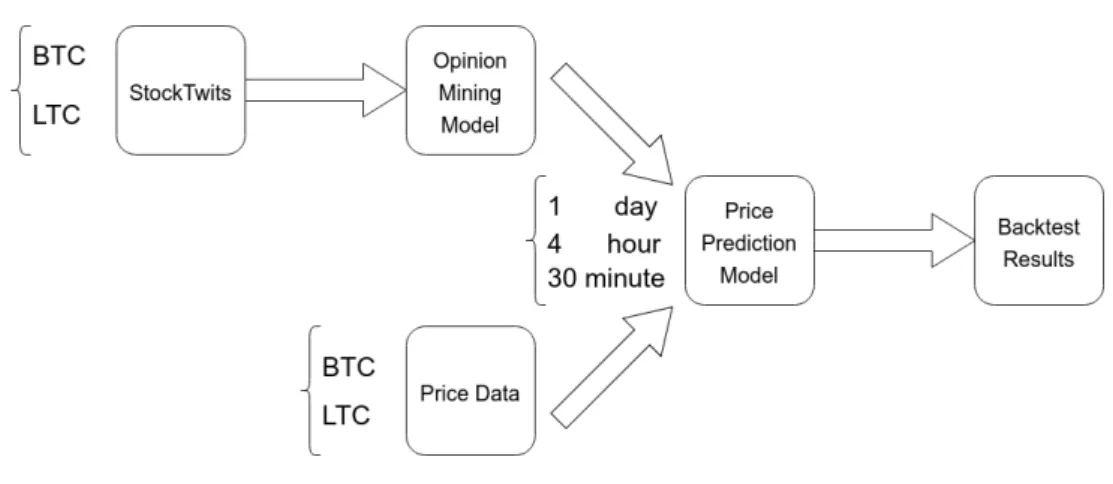
Figure 3.1: Architecture

In Figure3.1, the general architecture for the system built is presented.

StockTwits is used as a data source for cryptocurrency microblog data. This data is then used as input to opinion mining models which will label the opinion value regarding each specific cryptocurrency during a certain time period.

This opinion value is then combined with the corresponding price data for that time period and used as input for a price prediction model. This price prediction model is built in two ways, one with and one without the opinion values.

After building the price prediction model, a simple backtesting strategy is used to calculate the %-ROI each model would have produced if executed during the whole year of 2017.

The choice of using 3 different timeframes, 30 minute, 4 hour and 1 day is made to emulate three kinds of traders, day traders, swing traders and investors.

In order to compare the results obtained by the deep learning models with typical traders, mechanical trading strategies are also backtested for the year of 2017, so the different strategies’ %-ROI can me compared.

Conceptual Model

In this chapter, the choices for data sources, algorithms and benchmark are explained in detail.

3.2

Cryptocurrencies

The first step was to decide which currencies to analyze. The criteria used to choose cryptocur-rencies were:

• Cryptocurrencies which can be shorted on exchanges such as BitMEX [Bit18b] and Bitfinex [Bit18a], so the model can profit from both uptrends and downtrends

• Cryptocurrencies with a longer history of price action

• Cryptocurrencies with large market cap and high daily trading volume Taking these criteria into account, the chosen cryptocurrencies were: 1. Bitcoin (BTC)

2. Litecoin (LTC)

Both of these currencies meet the desired criteria.

All collected data reports to a period between 2015/08/07 and 2018/01/01.

3.3

Data Sources

3.3.1 Price Data

Price data of the chosen cryptocurrencies is collected using the Poloniex [Pol18] exchange histor-ical data API, which contains data for both chosen cryptocurrencies from 2015/08/07.

3.3.2 Opinion Mining

For the opinion mining layer of the architecture, two different data sources are used. One is a la-beled dataset to train the opinion mining algorithms and the other is a microblog dataset regarding the chosen currencies.

3.3.2.1 Labeled Dataset

The labeled data set is a modification of the Sem-Eval2017 Task 5 Fine-Grained Sentiment Anal-ysis on Financial Microblogs and News [RFN17]. The original dataset was improved to include opinion heavy cryptocurrency related slang and is available on github [Dat18]

3.3.2.2 Cryptocurrency Microblog

To construct a cryptocurrency microblog dataset, the StockTwits [Sto18b] API is used to collect Twits for the chosen cryptocurrencies using the StockTwits tickers BTC.X, ETH.X, LTC.X, XRP.X

Conceptual Model

3.4

Preprocessing

For each cryptocurrency, three different models are built for three diferent time frames: • 1 day

• 4 hour • 30 minute

This allows for three very different trading frequencies while maintaining a meaningful amount of available data.

For this, after data collection, both StockTwits and price data are aggregated into three different datasets, corresponding to each of the timeframes.

3.4.2 StockTwits

In order to format StockTwits text data to a fixed shape to use as input to deep learning models, the following pre-trained word are used:

• word2vec [MCCD13] • fastText [JGBM17] • GloVe [PSM14]

All three embeddings are used with 300 dimensions for each word.

3.5

Algorithms

3.5.1 Opinion Mining

For opinion mining, two different main algorithms are used, both of which were used by Bloomberg’s sumbmission for SemEval2017 Task 5 [RFN17].

These two algorithms were chosen as they have been proven to provide good results for the desired task.

Both algorithms are then tested with the three word embeddings.

Opinion mining in this work is tackled as a regression problem, instead of classification. As such, the activation function used on models is the rectified linear unit (ReLU), instead of the softmax function.

Conceptual Model

3.5.1.1 Convolutional Neural Network (CNN)

The architecture used is very similar to Cliche [Cli17], which in turn is similar to work published by Kim [Kim14]

Figure 3.2: Simplified architecture of the CNN used. Figure is taken from Cliche [Cli17]

Figure3.2represents a simplified, smaller version of the model used.

The network’s inputs are tokenized twits using the previously mentioned word embeddings, mapping twits to matrices of size s∗d, where s is the number of words in a twit and d the dimension of embedding space. The values chosen are s = 25 and d = 300. Zero padding is used to shape all twits into 25 ∗ 300 matrices.

Instead of 2 classes, the output generated is a continuous opinion measure in a [−1, 1] interval. 18

Conceptual Model

3.5.1.2 Bi-directional Long Short-Term Memory (LSTM) The architecture used is very similar to Cliche [Cli17].

Figure 3.3: Simplified architecture of the LSTM used. Figure is taken from Cliche [Cli17]

Figure3.2represents a simplified, smaller version of the model used.

Similar to the CNN model, the inputs to the LSTM are also tokenized twits using the chosen word embeddings, represented as 25 ∗ 300 matrices.

The LSTM model is used due to its capability to solve the diminishing and exploding gradients problem [HS98] found in simple Recurrent Neural Networks (RNN), by using a forget gate.

The Bi-directional LSTM is chosen since the regular LSTM only reads the sentence in one direction, thus not taking into account post word information. The Bi-directional LSTM solves this issue by having two different LSTMs reading the sentence forward and backward and then concatenating their hidden states.

Conceptual Model

3.5.2 Price Prediction

For price prediction, two different models are used, which are then combined with the multiple outputs from the opinion mining layer.

Figure 3.4: Japanese Candlestick. Figure is taken from [inv18a]

A japanese candlestick has an Open High Low Close (OHLC) format, indicating the price for those 4 values during the time period of the candlestick. Another value used for price prediction is Volume. In this case, Volume is the amount of coins traded in the time period of a candlestick. As such, the time format used for price prediction models is Open High Low Close Volume (OHLCV). For price prediction, a regression problem is tackled, attempting to predict the close price of the next candlestick, instead of a classification problem with two classes representing price going up or down.

3.5.2.1 LSTM

A one layer LSTM model is used.

As with opinion mining, the LSTM is used due to its ability to solve the exploding and dimin-ishing gradients problem, and because, as a RNN, it achieves superior results when analyzing time series data, such as price data.

Conceptual Model

3.5.2.2 State Frequency Memory (SFM)

SFM is a state of the art model introduced in 2017 [ZAQ17] specifically built for stock price prediction, which can also be used for cryptocurrency, commodities and foreign exchange.

Figure 3.5: SFM architecture. Figure is taken from [ZAQ17]

SFM tries to address the issue of dealing with time series of prices being non-stationary and non-linear. It is inspired by the discrete Fourier transform, and decomposes hidden states of mem-ory cells into frequency components. Future prices are then predicted as a nonlinear mapping of the cells in an inverse Fourier transform.

Modeling different frequencies can enable more accurate predictions for different time frames. The SFM is chosen due to it being a novel model built for price prediction.

Conceptual Model

3.6

Benchmarking

3.6.1 Opinion Model

In order to benchmark the opinion models on the SemEval2017 Task 5 dataset, the Mean Squared Error (MSE) as the loss function, instead of accuracy, since a regression model is used to assign an opinion value for each twit, instead of a classification model.

Models are not benchmarked against other SemEval2017 Task 5 submissions, as the used dataset is a modification of the original SemEval2017 Task 5 dataset, and the models used were used in a submission for the challenge itself.

3.6.2 Price Prediction

Price prediction models will be benchmarked against buying and holding, as well as classical mechanical trading strategies. The mechanical trading strategies were backtested using Trad-ingView’s [Tra18] backtesting functionalities, since TradingView allows for strategy backtesting using their proprietary programming language, PineScript [Pin18].

3.6.2.1 Exponential Moving Average (EMA) crossover

Figure 3.6: Moving Average Crossover Strategy. Figure is taken from [the18]

Conceptual Model

On a given period, the EMA is the exponential average of the last n periods. The exponential average is used to assign more weight to the most recent periods, so the moving average adjusts itself faster.

An EMA crossover occurs when two EMA’s cross each other. Whenever the faster moving average crosses above the slower moving average, a buy signal is generated, while a sell signal is generated when the opposite happens.

The chosen EMA crossover strategy is (20, 40)

3.6.2.2 Moving Average Converge Divergence (MACD) Crossover

Figure 3.7: MACD Crossover Strategy. Figure is taken from [onl18]

The MACD crossover strategy is similar to the EMA crossover strategy. The two lines used in this strategy are the MACD, calculated by subtracting the 26-period EMA from the 12-period EMA and the MACD-signal line, calculated as a 9-period EMA of the MACD.

Whenever the MACD crosses above the MACD signal line, a buy signal is generated, while a sell signal is generated when the opposite occurs.

Conceptual Model

3.6.2.3 Relative Strength Index (RSI) overbought & oversold

Figure 3.8: RSI Overbought Oversold Strategy. Figure is taken from [mql18]

The RSI is a momentum indicator bounded between in the [0, 100] interval. High values represent strong buy momentum while low values represent strong sell momentum.

The RSI is calculated diving the average of upward price change by the average of the down-ward price change, in the last 14 periods.

RSI values above 70 are considered overbought and values below 30 are consider oversold. A buy signal is generated when RSI below 30 returns to above 30 and a sell signal is generated when RSI above 70 returns to below 70.

Conceptual Model

3.6.2.4 Parabolic Stop and Reverse (SAR)

Figure 3.9: Parabolic SAR Strategy. Figure is taken from [inv18b]

When price is in an uptrend, the Parabolic SAR emerges below the price and converges towards it. It is calculated using the previous day’s parabolic SAR and the highest value on the current uptrend or the lowest value in the current downtrend.

Whenever price in a downtrend crosses above the Parabolic SAR, a buy signal is generated and whenever price in an uptrend crosses below the Parabolic SAR, a sell signal is generated.

Conceptual Model

Chapter 4

Implementation

This chapter provides an explanation of how the project was implemented. Specifying what tech-nology was used and how algorithms were used and how experiments were performed.

4.1

Data Collection

For text data collection, a NodeJS script was used to collect and structure twits referring to the selected cryptocurriences’ tickers, using the StockTwits NodeJS API.

As previously mentioned, the timeframe for collected StockTwits is from 2015/08/07 to 2018/01/01. After collecting the data, there are

• 500,000 BTC Twits • 200,000 LTC Twits

4.1.2 Price Prediction

In order to collect historical price data, another NodeJS script was used to collect cryptocurrency price data using the Poloniex REST API.

As previously mentioned, the timeframe for collected price data is from 2015/08/07 to 2018/01/01, with 2015/08/07 to 2017/01/01 being used as training data and 2017/01/01 to 2018/01/01 being used as testing data.

4.2

Preprocessing

Each twit was preprocessed according to the following rules • URLs are removed

Implementation

• Non alphanumeric characters are removed

• Any sequence of characters repeated more than 2 times is replaced by 2 repetitions of that sequence ("hahaha" is replaced by "haha")

• English stopwords included in python’s nltk package’s corpus are removed

After preprocessing, each preprocessed twit is converted, using one of the three chosen pre-trained word embeddings, word2vec FastText GloVe, which convert each word to a vector with 300 elements. After converting each word, a zero padding strategy is used for each twit, keeping each twit’s number of words to 25. As such, each twit is now represented as a 25 ∗ 300 matrix. When a twit’s number of words is lower than 25, vectors with dimension of 300, filled with zeros, are added to the matrix, to make sure its size is 25 ∗ 300.

4.2.2 Price Prediction

Before being used as input for deep learning models, price data is scaled in two ways, using scikit-learn’s MinMaxScaler.

Each cryptocurrency’s entire OHLC data is scaled to the [0, 1] interval. For the Volume part of the OHLCV data, there is a separate scaling done as for some cryptocurrencies, the volume is many orders of magnitude greater than the price.

4.3

Training

Deep learning models and building blocks used are from Google’s Keras [Ker18]. Keras is a high level API for Machine Learning and Deep Learning, which allows for rapid prototyping and testing, using Google’s TensorFlow [Ten18] as a back-end.

4.3.1 Opinion Mining

For opinion mining, two types of models are be used, a CNN and a Bi-directional LSTM.

As previously mentioned, the CNN model is very similar to the one depicted on Figure3.2, while the Bi-directional LSTM model is very similar to the one on Figure3.3

For training, a batch size of 8 is used, as well as 100 epochs. The training to testing set ratio is 0.75.

ReLU activation is on both models used as opinion mining in this work is tackled as a regres-sion problem, rather than classification.

For training, and testing, the Adam optimizer is used and the performance of the model is measured with the Mean Squared Error (MSE) metric, which measures the average of the squares of the errors, which are calculated as the difference between the predicted and the actual values.

Three types of models are trained using three different variations of the dataset, with each variation being the corresponding word embedding of the original dataset.

Implementation

For each variation of the dataset, different models are trained, making combinations of reg-ularization and dropout. Keras allows the Convolutional layers to have kernel, bias and activity regularization and the LSTM layers to have kernel, bias, activity and recurrent regularization.

During the experiments, different models having None, L1 and L2 regularization are used. Since a dropout layer is also used before the ReLU function, different models having 0.2, 0.5 and 0.8dropout are also used. For the LSTM model, different number of units are also tested, 5, 50 and 100.

To prevent one time models having a better result than the others, each specific model is trained and tested 20 times. For these 20 runs, the minimum and mean MSE error is recorded. Afterwards, results from all combinations are recorded and for each word embedding, the model with the lowest mean MSE is saved to use later in conjunction with price action data and StockTwits as the training and testing data used for Opinion Mining is not the data that will be used later to classify opinion for cryptocurrencies, it is only a modified version of the SemEval 2017 Task 5 dataset used to build the Opinion Mining models.

Below, the pseudo-code used for testing different combinations of hyper parameters and word embeddings on the LSTM model is presented. For the CNN model, a similar execution is per-formed, excluding the combinations of different numbers of units.

Implementation

Algorithm 1 LSTM Opinion model training pseudo-code

1: batch_size← 8

2: train_ratio← 0.75

3: epochs← 100

4: runs← 20

5: embeddings← [fasttest, glove, word2vec]

6: regularizers← [None, L1, L2]

7: units← [5, 50, 100]

8: for embedding in embeddings do

9: data← load_data(embedding) . Loads modified SemEval dataset

10: train, test← split_data(data, train_ratio)

11: best_mean← Infinity

12: best_min← Infinity

13: for dropout in dropouts do

14: for regularizer in regularizers do

15: for unit_number in units do

16: i← 0

17: results← []

18: while i < runs do

19: i← i + +

20: model← build_model(dropout, regularizer, unit_number)

21: model.train(train)

22: mse← model.test(test)

23: results.append(mse)

24: mean← get_mean(results)

25: min← get_min(results)

26: if mean < best_mean then

27: best_mean← mean

28: if min < best_min then

29: best_min← min

Implementation

After training the Opinion mining models on the modified Sem-Eval dataset, different versions of the price data dataset are created, each with different opinion values corresponding to different opinion mining models. In order to calculate the opinion value corresponding to given time period, or candlestick, the average of twits’ opinion value is calculated.

Algorithm 2 Opinion value calculation

1: cryptocurrencies← [BTC, LTC]

2: opinion_algos← [CNN, LSTM]

3: embeddings← [word2vec, glove, fasttext]

4: timeframes← [1, 4, 30]

5: for currency in cryptocurrencies do

6: for timeframe in timeframes do

7: price_data← load_price_data(currency, timeframe

8: twit_data← load_twit_data(currency, timeframe

9: for opinion_algo in opinion_algos do

10: for embedding in embeddings do

11: model← load_model(embedding, opinion_algo)

12: i← 0 13: while i < len(price_data) - 1 do 14: candlestick← price_data[i] 15: twits← twit_data[i] 16: opinion← 0 17: count← 1

18: for twit in twits do

19: twit← twit_to_vector(twit, embedding)

20: score← model.predict(twit)

21: opinion← ((count - 1) * opinion + score) / count

22: count← count + 1

23: if count == 0 & i > 0 then

24: opinion← price_data[i - 1].opinion

25: price_data[i].opinion← opinion

26: save_data(price_data, currency, timeframe, opinion_algo, embedding)

4.3.2 Price Prediction

For price prediction, two types of models are be used, LSTM and SFM.

Both LSTM and SFM models use only one layer of each of the models, afterwards, dropout is used as well as ReLU activation.

For training, a batch size of 8 is used, as well as 50 epochs. Training data refers to the period from 2015/08/07 and 2017/01/01 and testing data refers to the period from 2017/01/01 to 2018/01/01.

The Adam optimizer is used and the performance of the model is measured with the Mean Squared Error (MSE) metric, which measures the average of the squares of the errors, which

Implementation

are calculated as the difference between the predicted and the actual values. To measure the performance, the %-ROI is also calculated.

In order to obtain the %-ROI, if the next candlestick close prediction is above the current, a long position is taken and a short position otherwise. This strategy performs one trade every can-dlestick, this strategy may lead to worse results as trades are usually held for multiple candlesticks. Algorithm 3 %-ROI calculation pseudo-code

1: roi← 100

2: model← load_price_model()

3: data← load_price_data() . Test price data, relative to the year of 2017

4: i← 0 5: while i < len(data) - 1 do 6: current← data[i] 7: next← data[i + 1] 8: current_close← current.close 9: next_close← next.close 10: predicted← model.predict(current) 11: long← -1

12: if predicted > current_close then

13: long← 1

14: factor← (1 + (short * (next_close - current_close) / current_close))

15: roi← roi * factor

16: model.fit(current, next) . After using the current candlestick to calculate %-ROI, re-train the model with it. Similar to an online learning approach

17: i← i + +

Similar to the Opinion Mining models, different models are trained, making combinations of regularization and dropout. Both LSTM and SFM may have kernel, bias, activity and recurrent regularization. The SFM model is not included in the Keras package. The implementation used can be found on GitHub [SFM18]

During the experiments, different models having None, L1 and L2 regularization are used. Since a dropout layer is also used before the ReLU function, different models having 0.2, 0.5 and 0.8 dropout are also used. For the LSTM model, different number of units are also tested, 5, 50 and 100.

To prevent one time models having a better result than the others, each specific model is trained and tested 10 times. For these 10 runs, the minimum and mean MSE error is recorded. Afterwards, results from all combinations are recorded and for each word embedding, the model with the lowest mean MSE is saved to use later in conjunction with price action data and StockTwits as the training and testing data used for Opinion Mining is not the data that will be used later to classify opinion for cryptocurrencies, it is only a modified version of the SemEval 2017 Task 5 dataset used to build the Opinion Mining models.

Two types of price prediction datasets are used. One is only the OHLCV data while the other one includes the an opinion value for each candlestick, generated by the Opinion Mining models. This way, it is possible to measure the benefit of adding the opinion value for prediction.

Implementation

Below, the pseudo-code used for testing different combinations of hyper parameters and dif-ferent opinion values from difdif-ferent word embeddings on the LSTM model is presented. For the SFM model, a similar execution is performed, excluding the combinations of different numbers of units.

For the original OHLCV dataset, without opinion values, a similar executed is performed, excluding the combination of word embedding opinion values.

Implementation

Algorithm 4 LSTM Price Prediction model training pseudo-code

1: batch_size← 8 2: epochs← 50 3: runs← 10 4: regularizers← [None, L1, L2] 5: units← [5, 50, 100] 6: dropouts← [0.2, 0.5, 0.8] 7: cryptocurrencies← [BTC, LTC] 8: opinion_algos← [CNN, LSTM]

9: embeddings← [word2vec, glove, fasttext]

10: for opinion_algo in opinion_algos do

11: for embedding in embeddings do

12: for currency in cryptocurrencies do

13: data← load_data(currency, embedding, opinion_algo)

14: train, test← split_data(data)

15: best_mse_mean← Infinity

16: best_mse_min← Infinity

17: best_profit_mean← Infinity

18: best_profit_min← Infinity

19: for dropout in dropouts do

20: for regularizer in regularizers do

21: for unit_number in units do

22: i← 0

23: mse_results← []

24: profit_results← []

25: while i < runs do

26: i← i + +

27: model← build_model(dropout, regularizer, unit_number)

28: model.train(train) 29: mse← model.test(test) 30: profit← get_profit(test) 31: mse_results.append(mse) 32: profit_results.append(profit) 33: mse_mean← get_mean(mse_results) 34: mse_min← get_min(mse_results)

35: if mse_mean < best_mse_mean then

36: best_mse_mean← mse_mean

37: if mse_min < best_mse_min then

38: best_mse_min← mse_min

39: profit_mean← get_mean(profit_results)

40: profit_min← get_min(profit_results)

41: if profit_mean < best_profit_mean then 42: best_profit_mean← profit_mean

43: if profit_min < best_profit_min then

44: best_profit_min← profit_min

Chapter 5

Results

This chapter provides the results obtained from performing the experiments described in the pre-vious chapter.

5.1

Opinion Mining

Below, the MSE results for the best hyper parameter configurations for both CNN and LSTM mod-els, using all three used word embeddings are presented. The data used is the modified SemEval dataset mentioned in previous chapters.

5.1.1 CNN

embedding mean min

word2vec 0.138 (0.2/l2) 0.123 (0.8/None) GloVe 0.159 (0.2/None) 0.159 (0.2/None) FastText 0.136 (0.2/l2) 0.131 (0.2/l2)

Table 5.1: CNN Opinion Model - MSE (dropout/regularizer)

Better results were observed for low dropout values on the CNN model, which was also the case in the work by [ZW15].

5.1.2 LSTM

embedding mean min

word2vec 0.131 (0.8/100/l2) 0.124 (0.8/100/None) GloVe 0.135 (0.8/100/None) 0.130 (0.5/100/None) FastText 0.125 (0.8/100/l2) 0.120 (0.8/100/l2) Table 5.2: LSTM Opinion Model - MSE (dropout/units/regularizer)

Results

As expected for an LSTM model, and contrary to a CNN model, high dropout values result in better results than lower dropout values.

5.1.3 Conclusion

The discrepancy between mean and min MSE values indicates that using a larger number of runs is justified to better analyze what is the best model.

It is also observed that for both CNN and LSTM using l1 and l2 regularization hardly has an impact MSE. If the dataset was larger, regularization could have had a more noticeable impact on results.

The LSTM model has obtained better results than the CNN model overall, with a larger differ-ence for the GloVe embedding.

5.2

Price Prediction

Below, the result for the mechanical trading strategies used to compare with the created models are presented, as well as the MSE and Profit results for the best hyper parameter configurations for both LSTM and SFM models are presented.

The data used for testing is the price data between 2017-01-01 and 2018-01-01.

5.2.1 Mechanical Strategies

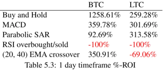
BTC LTC

Buy and Hold 1258.61% 259.28%

MACD 359.78% 301.69%

Parabolic SAR 92.69% 313.58% RSI overbought/sold -100% -100%

(20, 40) EMA crossover 350.91% -69.06%

Table 5.3: 1 day timeframe %-ROI

BTC LTC

Buy and Hold 1258.61% 259.28%

MACD 210.78% 263.61%

Parabolic SAR 790.79% 183.22% RSI overbought/sold -100% -100%

(20, 40) EMA crossover 537.62% 911.42% Table 5.4: 4 hour timeframe %-ROI

Results

BTC LTC

Buy and Hold 1258.61% 259.28%

MACD -92.17% -95.45%

Parabolic SAR 113.44% -97.11%

RSI overbought/sold -85.09% -100%

(20, 40) EMA crossover 2144.16% 1493.27% Table 5.5: 30 minute timeframe %-ROI

5.2.2 No opinion data

5.2.2.1 LSTM

Coin meanMSE minMSE meanPROFIT maxPROFIT

BTC 5.17e-4(100/0.8/l1) 4.83e-4(100/0.8/None) 16.05%(100/0.8/None) 107.55%(100/0.8/None) LTC 1.93e-3(100/0.8/None) 1.87e-3(50/0.5/None) -65.71%(100/0.8/l1) -58.97%(100/0.8/l1)

Table 5.6: 1 day LSTM(units/dropout/regularizer)

Coin meanMSE minMSE meanPROFIT maxPROFIT

BTC 2.48e-3(100/0.8/None) 2.39e-3(100/0.8/l2) 37.90%(100/0.8/None) 103.47%(100/0.8/None) LTC 3.25e-4(100/0.8/None) 3.13e-4(100/0.8/None) -49.83%(100/0.8/l2) -6.90%(100/0.8/l2)

Table 5.7: 4 hour LSTM(units/dropout/regularizer)

Coin meanMSE minMSE meanPROFIT maxPROFIT

BTC 7.23e-3(100/0.8/None) 6.72e-3(100/0.8/None) 51.22%(100/0.8/None) 131.18%(100/0.8/None) LTC 5.33e-4(100/0.8/None) 4.82e-4(100/0.8/None) -30.98%(100/0.8/l2) 22.43%(100/0.8/None)

Table 5.8: 30 minute LSTM(units/dropout/regularizer)

From these results, we can observe that there isn’t a strong relationship between MSE and obtained Profit. Also, the model accomplished better results on lower time frames.

As with the previous opinion mining models, the LSTM has better results with a higher amount of units and high dropout, while regularization did not have a significant impact on results.

Results

5.2.2.2 SFM

Coin meanMSE minMSE meanPROFIT maxPROFIT BTC 6.67e-2(0.8/None) 5.49e-2(0.8/None) -68.11%(0.8/None) -48.15%(0.5/l2) LTC 2.88e-3(0.8/None) 1.68e-3(0.8/None) -52.83%(0.5/l1) 12.00%(0.5/l1)

Table 5.9: 1 day SFM(dropout/regularizer)

Coin meanMSE minMSE meanPROFIT maxPROFIT BTC 1.29e-2(0.8/l2) 1.98e-3(0.8/None) 31.08%(0.8/l2) 368.43%(0.8/l1) LTC 5.42e-4(0.8/None) 3.23e-4(0.8/l1) -28.27%(0.8/l1) 111.72%(0.8/None)

Table 5.10: 4 hour SFM(dropout/regularizer)

Coin meanMSE minMSE meanPROFIT maxPROFIT BTC 4.17e-2(0.8/l1) 8.32e-3(0.8/None) 45.28%(0.8/None) 253.56%(0.8/l1) LTC 1.12e-3(0.8/None) 7.56e-4(0.8/None) 11.09%(0.8/l2) 202.44%(0.8/None)

Table 5.11: 30 minute SFM(dropout/regularizer)

From the results, we observe that like for the LSTM model, there isn’t a strong relationship be-tween MSE and profit and that the model achieved better results on lower timeframes with a higher dropout value.

What can be noted is that the SFM model achieves better results than the LSTM overall.

5.2.3 Opinion data

5.2.3.1 LSTM

Coin meanMSE minMSE meanPROFIT maxPROFIT BTC 8.04e-3 2.58e-3 35.55% 154.65%

(100/0.8/None/ (100/0.5/l1/ (100/0.8/None/ (100/0.8/l2/ fasttext/CNN) glove/LSTM) word2vec/LSTM) glove/CNN) LTC 2.63e-3 2.18e-3 -11.64% 25.08%

(100/0.8/l2/ (100/0.8/l2/ (100/0.8/None/ (100/0.8/l2/ word2vec/LSTM) glove/CNN) fasttext/LSTM) glove/CNN) Table 5.12: 1 day LSTM Opinion(units/dropout/regularizer/embedding/opinion)

Results

Coin meanMSE minMSE meanPROFIT maxPROFIT BTC 1.91e-2 1.63e-2 66.94% 222.27%

(100/0.8/l1/ (100/0.8/None/ (100/0.8/None/ (100/0.8/l2/ glove/CNN) glove/CNN) word2vec/CNN) glove/LSTM) LTC 5.59e-4 3.8e-4 23.73% 85.19%

(100/0.5/l1/ (100/0.8/l2/ (100/0.8/None/ (100/0.8/None/ t glove/CNN) glove/LSTM) word2vec/LSTM) glove/CNN) Table 5.13: 4 hour LSTM Opinion(units/dropout/regularizer/embedding/opinion)

Coin meanMSE minMSE meanPROFIT maxPROFIT BTC 0.23e-2 8.77e-3 73.15% 166.40%

(100/0.8/l1/ (100/0.8/None/ (100/0.8/None/ (100/0.8/l1/ glove/LSTM) glove/LSTM) word2vec/LSTM) glove/LSTM) LTC 3.33e-4 1.2e-4 31.09% 104.63%

(100/0.8/None/ (100/0.8/l1/ (100/0.8/k2/ (100/0.8/None/ word2vec/LSTM) word2vec/CNN) word2vec/LSTM) fasttext/CNN) Table 5.14: 30 minute LSTM Opinion(units/dropout/regularizer/embedding/opinion)

5.2.3.2 SFM

Coin meanMSE minMSE meanPROFIT maxPROFIT BTC 7.13e-2 6.73e-2 58.94% 170.94%

(0.8/None/ (0.8/l1/ (0.8/None/ (0.8/None/ word2vec/LSTM) word2vec/CNN) word2vec/LSTM) fasttext/CNN) LTC 7.54e-4 8.29-4 32.14% 133.89%

(0.8/l1/ (0.8/None/ (0.8/l1/ (0.8/None/ glove/LSTM) glove/LSTM) word2vec/LSTM) glove/LSTM) Table 5.15: 1 day SFM Opinion(dropout/regularizer/embedding/opinion)

Results

Coin meanMSE minMSE meanPROFIT maxPROFIT BTC 7.13e-2 6.82e-2 53.94% 250.94%

(0.8/None/ (0.8/l1/ (0.8/None/ (0.8/l2/ glove/CNN) glove/CNN) word2vec/CNN) glove/LSTM) LTC 8.34e-4 3.48e-4 66.14% 170.89%

(0.8/l2/ (0.8/None/ (0.8/None/ (0.8/None/ glove/CNN) glove/LSTM) word2vec/LSTM) glove/CNN) Table 5.16: 4 hour SFM Opinion(dropout/regularizer/embedding/opinion)

Coin meanMSE minMSE meanPROFIT maxPROFIT BTC 5.03e-2 2.12e-2 88.35% 185.79%

(0.8/None/ (0.8/l2/ (0.8/None/ (0.8/None/ word2vec/LSTM) glove/CNN) fasttext/LSTM) glove/CNN) LTC 5.71e-4 0.29e-4 105.14% 320.21%

(0.8/None/ (0.8/l1/ (0.8/l1/ (0.8/None/ fasttext/CNN) glove/LSTM) word2vec/LSTM) glove/CNN) Table 5.17: 30 minute SFM Opinion(dropout/regularizer/embedding/opinion)

The best model obtained was the SFM with opinion data, obtaining the following average returns: Coin 1 day 4 hour 30 min

BTC 58.94% 53.94% 88.35% LTC 32.14% 66.14% 105.14% Table 5.18: Best obtained model - SFM opinion data

Although these %-ROI returns are satisfactory, they are much lower than the best mechanical trading strategies for the year of 2017

Coin 1 day 4 hour 30 min BTC 350.91% 537.62% 2144.16% LTC -69.06% 911.42% 1493.27%

Table 5.19: Best mechanical strategy - (20, 40) EMA crossover