Demographic
history of the
isolated and
endangered wolf
population in the
South of Douro
river
Raquel Freitas Pedra Monteiro
Mestrado em Biodiversidade, Genética e Evolução
Departamento de Biologia2014/2015
Orientador
Raquel Godinho, Assistant Researcher, CIBIO/InBIO Invited Assistant Professor, FCUP
Coorientador
Francisco Álvares, Post-Doc Researcher, CIBIO/InBIO
Todas as correções determinadas pelo júri, e só essas, foram efetuadas. O Presidente do Júri,
Acknowledgements
I would like to thank my tutors and advisors: Raquel Godinho, Francisco Álvares and José Vicente López-Bao for giving me the opportunity to conduct this work and for the constant support and patience and for the innumerous hours spent helping me.
I would also would like to thank Diana Castro and Diana Lobo for allowing me to feel so welcomed in the laboratory and for teaching me so much.
Besides that, I also must thank my colleagues and friends for all the support, help and fun moments they provided in this last year.
In addition I would like to thank my family for giving me the opportunity to study and supporting me no matter what.
And lastly, I would like to thank to all the institutions and private collectors for donating the historical samples that were so important in this thesis: Estación Biológica de Doñana, Museu Nacional de História Natural e das Ciências, Reserva Natural da Serra da Malcata, Tapada de Mafra, Museu de Coimbra, Café “Vitória”, Clube de caça e pesca da Covilhã, Museu Municipal de Penamacor, Liceu Nuno Álvares, Colégio Padres Redentoristas, Jerónimo Trigueiros de Aragão, António Cabral Fialho (Herdade das Russianas), Francisco Borba (Herdade da Gambia), Francisco José Almeida Morgado Pavalhã, Lurdes Rodrigues
First cover photo: “Resultado de uma batida aos lobos, Idanha-a-Nova, década 1930 (© Arquivo Francisco Álvares/CIBIO)”
Abstract
The current small wolf population located at South of Douro river in Portugal has suffer a strong range decline during the last decades and become isolated from the main wolf population in Iberian Peninsula. This negative trend has led this wolf population, with a current estimate of less than 30 individuals, to the verge of extinction. In this setting, the Portuguese South Douro wolf population provides a perfect model to evaluate the demographic and genetic effects of a sharp decline in a large carnivore, providing valuable knowledge for current wolf management and conservation.
In our study we: i) tried to understand the genetic configuration of this population in the past, ii) compare the previous results to the genetic values obtained in the present population, iii) determine the range of the population in the past and see its evolution through time and iv) calculate the probability of wolf persistence.
To assess distribution trends, we used available presence records of wolves in Portugal since 1900 to estimate range extension, level of fragmentation, estimated population size, extinction rate and the probability of demographic persistence along the 20th century.
To assess genetic patterns as consequence of range decline, we used modern samples from the Portuguese wolf populations located both at South and Northern Douro river and historical samples only from the Southern population. By genotyping each individual we evaluated population structure, genetic diversity and effective population sizes for the historical and contemporary wolf populations.
With these two complementary approaches we arrived to similar conclusions. In the past, the South Douro population was much more diverse (Ho=0.307, while for the contemporary Ho=0.290), had an effective population size and a distribution area much higher than it has today (Historic population with Ne=40, contemporary population with Ne=15). Historical samples revealed that the past South Douro population was genetically similar to the contemporary North Douro population, this might indicate that these two populations have been connected in the past, and only recently, due to reduction in size, has the South Douro population become isolated. With the range regression that occurred, small fragments emerged which had a much higher risk of extinction due to the smaller number of wolves present in them. We can conclude that given the extensive persecution and habitat loss due to the increase in agriculture, the South Douro wolf population lost a great amount of genetic diversity and a great
number of individuals. Due to its isolation, nowadays this population faces a high risk of extinction.
Keywords:
Demography, distribution trends, effective population size, historical samples, Portugal, South of Douro wolf population, Wolf.
Resumo
A pequena população atual de lobos localizada a Sul do Douro em Portugal tem sofrido uma forte diminuição de área durante as últimas décadas e ficou isolada da população principal de lobos da Península Ibérica. Esta tendência negativa levou esta população de lobos, com uma estimativa atual de menos de 30 indivíduos, ao limite da extinção. Com este cenário, a população portuguesa de lobos a Sul do Douro providencia um modelo perfeito para avaliar os efeitos demográficos e genéticos de um declínio acentuado num carnívoro grande, providenciando um conhecimento valioso para a atual gestão e conservação do lobo.
No nosso estudo: i) tentamos entender a configuração genética desta população no seu passado, ii) comparar os resultados anteriores com os valores genéticos obtidos na população presente, iii) determinar o tamanho da população no passado e ver a sua evolução ao longo do tempo e iv) calcular a probabilidade da persistência do lobo.
Para aferir as tendências da distribuição, usamos registos de lobos disponíveis em Portugal desde 1900 para estimar o tamanho da extensão, nível de fragmentação, tamanho estimado da população, velocidade de extinção e a probabilidade de persistência demográfica durante o século 20.
Para avaliar padrões genéticos como consequência do declínio do tamanho, usamos amostras modernas de populações de lobo portuguesas localizadas ambas a Sul e Norte do rio Douro e amostras históricas apenas da população do Sul. Ao genotipar cada indivíduo avaliámos a estrutura da população, diversidade genética e o tamanho da população efetiva para as populações de lobo histórica e contemporânea.
Com estas duas metodologias chegamos a conclusões semelhantes. No passado, a população do Sul do Douro era muito mais diversificada, tinha um tamanho efetivo de população e área de distribuição muito maior do que hoje. Amostras históricas revelam que a população do Sul do Douro do passado era geneticamente semelhante à população contemporânea do Norte do Douro, isto pode indicar que estas duas populações estiveram conectadas no passado, e apenas recentemente, devido à redução em tamanho, a população do Sul do Douro se tornou isolada. Com esta regressão de tamanho, pequenos fragmentos apareceram, o que teve um risco mais alto de extinção devido ao reduzido número de lobos presente neles. Podemos concluir que dada a extensiva perseguição e perda de habitat devido à agricultura, a população de lobo do Sul do Douro perdeu uma grande parte de diversidade genética
e um grande número de indivíduos. Devido à sua isolação, atualmente esta população enfrenta um alto risco de extinção
Palavras-chave:
Amostras históricas, demografia, lobo, população de lobos do Sul do Douro, Portugal, tamanho efetivo populacional, tendências de distribuição.
Table of contents
Acknowledgements ... 3 Abstract ... 4 Keywords: ... 5 Resumo ... 6 Palavras-chave: ... 7 Table of contents ... 8 Figure contents ... 10 Table contents ... 12 1. Introduction ... 131.1- Demographic history and implications to wildlife conservation ... 13
1.2. The usefulness of historical samples and genetic tools ... 14
1.3. – Insights from wolves in the Iberian Peninsula ... 18
Objectives ... 21
Materials and Methods ... 22
Study area ... 22
Distribution trends ... 22
Molecular patterns ... 24
Sample collection ... 24
DNA extraction... 25
Ancient DNA extraction protocol ... 26
Blood and Tissue Extraction kit ... 27
DNA Quantification ... 27
EzRAD for SNPs discovery ... 28
Choosing the restriction enzymes... 28
Library preparation ... 29
Library enrichment ... 31
Illumina HiSeq Run and data analysis ... 31
Genotyping previously known SNPS ... 32
Results ... 35
Distribution trends ... 35
Range patterns, fragmentation and estimate population size ... 35
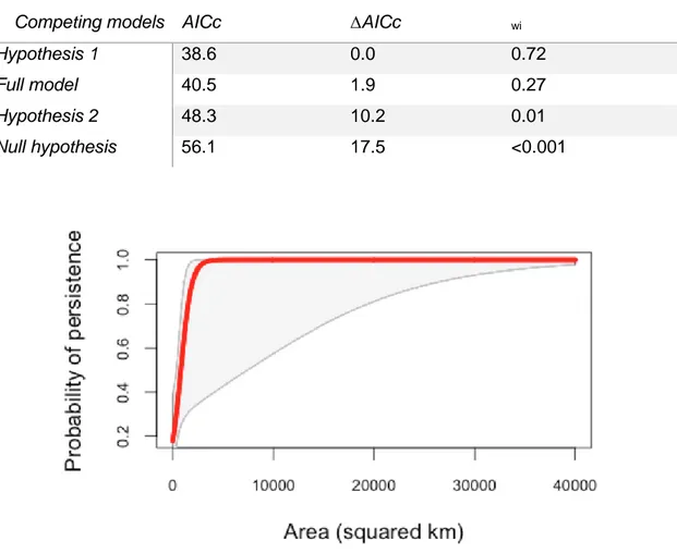
Persistence probability ... 39
Trends on habitat conditions within wolf range ... 40
Molecular patterns ... 41
DNA Extraction analysis ... 41
EzRAD analysis ... 42
SNPs diversity ... 44
Discussion ... 52
Distribution patterns: insights from a strong population decline ... 52
Molecular markers and tools: challenges from historical samples ... 53
Genetic patterns: a historical and contemporary view of wolf populations in Portugal ... 56
Conclusion and future work... 58
References ... 59
Figure contents
Figure 1- Wolf distribution and detected packs in Iberian Peninsula, with a red square representing the South Douro river wolf population in Portugal (adapted from Alvares, et al. (2005) ... 19 Figure 2-Assembly performed in the extraction protocol A-Labeld MinElute spin
columns B- Zymo extension reservoirs C-Assembly of columns and reservoirs D-Assembly inside de 50mL falcon tube. E-D-Assembly with sample and binding buffer inside. ... 26 Figure 3- Sample order in agarose gel. Each gel had two ladders in the extremities and five samples, always separated by one well to avoid cross-contamination. ... 30 Figure 4-Models tested in DIYABC. The first model is the null hypothesis, the second one suggests that historical samples were taken before the bottleneck that occurred in the South of Douro population, and the third model assumes historical samples were taken while the bottleneck was occurring. We assumed that the North of Douro
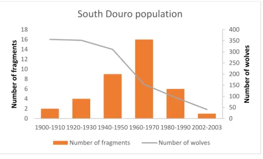
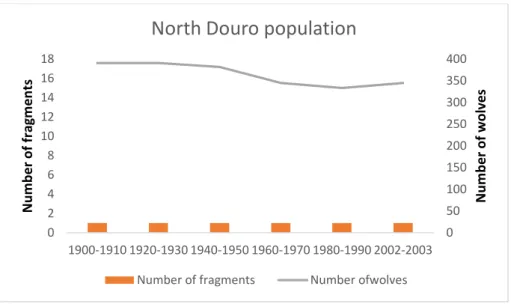
population maintained its size. ... 34 Figure 5-Wolf distribution between 1900 and 2003 represented in 10x10km squares. Level of fragmentation considering two different buffers of wolf dispersion distances, a 30km buffer (light blue) and a 50km buffer (dark blue). ... 36 Figure 6 Number of presence fragments and estimated wolves in the South Douro population from 1900 to 2003. The fragments were considered isolated when the nearest wolf presence was located more than 10km apart. The number of wolves in each fragment was based in current values of wolf density (see Methods section for details). ... 37 Figure 7 - Number of presence fragments and estimated wolves in the North Douro population from 1900 to 2003. The fragments were considered as adjacent 10x10km squares with wolf presence located more than 10km apart from the nearest one. The number of wolves in each fragment was based in current values of wolf density (see Methods section for details). ... 38 Figure 8 - Area of wolf range (blue columns) in the South Douro population and
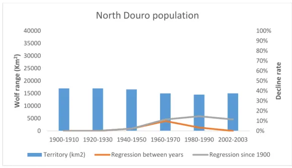
regression rate between years (orange line) and since the begining of the 20th century (grey line). ... 38 Figure 9 - Area of wolf range (blue columns) in the North Douro population and
regression rate between years (orange line) and since the beginning of the 20th
Figure 10 - Probability of fragment persistence in relation to fragment size (area in km2). Shaded area represents SE. ... 40 Figure 11 - Temporal trends of agricultural area (in Km2) in wolf range at North and South Douro river throughout the 20th century... 41 Figure 12 - Temporal trends of livestock numbers (in nº of animals) in wolf range at North and South Douro river area throughout the 20th century. ... 41 Figure 13 - Libraries after gel extraction and PCR enrichment. First 23 samples are modern samples and the following are historic samples. When no band is present the library enrichment was unsuccessful. ... 43 Figure 14 - Individual observed heterozygosity of the wolf samples through time from different locations in the South Douro river. Results for the contemporary North Douro river samples is also presented. ... 46 Figure 15 - Observed (Ho) and expected heterozygosity (He) in the three subsets of wolf samples (historic (H), contemporary south population (SD), contemporary north population (ND)) and dogs. ... 46 Figure 16 - Number of alleles present in the three groups of wolf samples (historic (H), contemporary south population (SD) and contemporary north population (ND)) and dogs. ... 47 Figure 17 - Private alleles (blue) and rare alleles (orange) presented in historic samples and modern samples of the southern population and in contemporary northern
population. ... 47 Figure 18 - Assignment of individuals to K populations. The results show that the more probable division is K=3. ... 48 Figure 19 - Probabilistic assignment to two genetic clusters, K=2 (A), and three genetic clusters, K=3 (B) inferred by the Bayesian analysis of wolf historical and modern samples. Each individual is represented by a vertical line fragmented in two sections that are relative to their membership proportion in respective genetic cluster... 49 Figure 20 -Structure results for K=2. Samples are represented by pie charts with the probabilistic assignment to two genetic clusters (K=2). Historic samples have a brown outline, northern samples have dark blue outline and southern samples have dark green outline. ... 50 Figure 21 - Structure results for K=3. Historic samples have a brown outline, northern samples have dark blue outline and southern samples have dark green outline. ... 51
Table contents
Table 1-Samples used in this study and their origin, location and type. EBD-Estación Biológica de Doñana, MNHNC-Museu Nacional de História Natural e das Ciências, RNSM-Reserva Natural da Serra da Malcata, SMLM- Sistema de monitorização de Lobos Mortos. ... 25 Table 2-Hypothesis and their AIC and akaike weight. Hypothesis 1 represents the hypothesis where the area influences the extinction of a fragment. Hypothesis 2 represents the risk of fragment extinction when there is few and far fragments away. Full model includes all the predictors pooled. ... 40 Table 3-In silico digestions of the dog genome with 17 restriction enzymes using
SimRAD. Restriction enzymes characteristics and results for the number of cuts and the number of fragments with the two different sizes tested, 100 to 150 base pairs and 210 to 260 base pairs. ... 42 Table 4-Average alignment in different types of samples (modern vs historical, private collections vs museum collections and historical bone samples vs historical tissue samples). ... 43
1. Introduction
1.1- Demographic history and implications to wildlife conservation
Rapid declines in the size of a population, named as bottlenecks, tend to cause a reduction in genetic variation, due to higher genetic drift (Nyström, et al. 2006; Reed 2005). Loss of genetic variation can increase the risk susceptibility of a population leading it to loss of fitness and, consequently, to a decrease in the chance of survival in a changing environment (Reed 2005). A small population can additionally suffer from inbreeding, reducing even more its genetic diversity and average individual fitness, resulting in inbreeding depression, ultimately leading to the fixation of recessive deleterious mutations (Lande 1988; Palstra and Ruzzante 2008).Besides small population size, the demographic trend of a population can also be influenced by fragmentation, especially when this causes absence of gene flow. Population size has a major impact on the dynamics of a population. It is thus of first importance to estimate the effective population size. Effective population size (Ne) refers to the size of an ideal population that is experiencing the same amount random genetic change as the population under consideration (Crow and Kimura 1970; Holleley, et al. 2014). Effective population size differs from census population size (Nc) the number of individuals accounted in a population, being Ne normally smaller. The ratio between Ne and Nc has been estimated to be 0.5 but it can change with variations in population size, unequal sex rations, inconsistency in reproductive success leading to a much smaller Ne. Fluctuations in population size can reduce Ne even further (Lande 1988; Palstra and Ruzzante 2008).
Estimating effective population size in endangered populations is crucial, because this measure affects directly the future of the population, influencing the response to selection and increasing inbreeding effect (Crow and Kimura 1970; Tallmon, et al. 2004), factors that increase the extinction risk. Estimating effective population size can, thus, help to predict the risk of extinction of a population, and then help to implement management strategies to mitigate those risks (Leberg 2005; Luikart, et al. 2010; Mace and Lande 1991). Some studies (McKay 1985) have estimated the effective size a population should have to survive, but this number is doubtful, because different species have different ecological behaviors that influence this number (Lande 1988). An Ne of 50 has been suggested to minimize inbreeding (Soule and Wilcox 1980). Nonetheless, estimating effective population size, through time and even before human pressure could help manage a population and give the number of individuals
needed to restore the population to its former abundance (Alter, et al. 2007). To access the dimension of the bottleneck and how diverse was a population, historical samples are needed (Nyström, et al. 2006; Pertoldi, et al. 2001).
Effective population size can be estimated through various genetic methods. One-sample estimators use data from one specific time and infer the effective population size based on the linkage between each locus or the heterozygote excess (Luikart, et al. 2010; Pudovkin, et al. 1996). Multiple-samples estimators use samples from at least two different times and use the change in allele frequencies to infer effective population size (Leberg 2005; Skrbinsek, et al. 2012; Tallmon, et al. 2004; Waples 1989). However, both methods are based in some assumptions like, for example, closed populations and discrete generations that not always correspond to the studied natural populations (Luikart, et al. 2010; Waples and Do 2008), leading to some bias in calculations. Many examples in the literature show that populations that have suffered past bottlenecks still show its effects today. The arctic fox (Alopex lagopus) described in Nyström, et al. (2006), a population that suffered a severe bottleneck in the 20th century, lost 25% of the microsatellites alleles. The case of the gray whales (Eschrichtius robustus), severely hunted in the 19th century, was estimated to have three to five times the census size it has nowadays (Alter, et al. 2007). So, for management situations estimating why, when, how and the severity of a past bottleneck event can give extensive tips in how a population can be protected (Cornuet and Luikart 1996). Bottleneck detection can be achieved using heterozygosity excess, M-ratio tests, or estimating the effective population size of a population through time. M-ratio tests as well as Ne estimated through linkage disequilibrium will be able to detect fairly recent bottlenecks, where heterozygosity excess will not (Luikart, et al. 2010). One thing that can disguise or even erase a bottleneck signal is immigration (Busch, et al. 2007). So, choosing the right method that best applies to the studied population is crucial in order to obtain good results.
1.2. The usefulness of historical samples and genetic tools
To study population trends along time is necessary to compile historical and present records of species presence. This information can then be used to calculate population size and range along a time period and compare them with contemporary values and information obtained from genetic markers. For that, we will need to access the genetic diversity using genetic markers, in this case, SNPs (short for Single Nucleotide Polymorphisms). It is possible to determine effective population size through time using only modern samples and inferring it to the past, however, if ancient
or historical samples exist, they will give a more accurate insight to the population’s history (Leonard 2008).
Historical DNA (hDNA) consists in samples of material previously collected and stored in a way not aimed on purpose for DNA extraction. The incorrect storage accelerates DNA degradation that will be of low quality and low quantity (Miller, et al. 2002; Navascués, et al. 2010). Naturally, reduced quantity and quality of DNA makes it more susceptible to contamination and more difficult to be amplified, especially for large fragments. Thus, extreme caution needs to exist when handling these samples, such as a room dedicated only for DNA extractions, a physically separated PCR (Polymerase Chain Reaction) room and several negative controls for extraction and PCR (Leonard 2008). When genotyping these samples, given their quality, errors are to be expected, possibly compromising the precision of the data (Miller, et al. 2002). Historical samples can be obtained from fur, pelts, bones or embalmed specimens in museum collections, or through private collections, especially when the species has been hunted. Samples from embalmed animals have additional problems since these have a plethora of chemicals infused that might have heavily degraded the DNA and diminish the probability of amplification with PCR. Private collections might also have further complications since samples are generally not stored properly.
Even though historic samples are difficult to extract DNA from, several studies have been successful in extracting and amplifying DNA fragments from ancient samples. By using samples with hundreds or even thousands of years old, several studies were able to infer population history in a wide number of contemporary or extinct species. Debruyne, et al. (2008) successfully extracted and amplified ancient DNA from 106 samples of wooly mammoths (Mammuthus primigenius) across their Holarctic range, inferring phylogeography and population history using mtDNA markers. Thalmann, et al. (2011), manage to study the demographic history of the Gorilla (Gorilla gorilla) by using ancient DNA extracted from teeth roots and successfully amplified microsatellites. Similarly, ancient samples, as bone and teeth, have also been used to study wolf populations and even the origin of the new world dogs by extracting DNA and amplifying the mitochondria control region (Leonard, et al. 2005; Leonard, et al. 2002). These examples show that historic and ancient DNA can be very useful for phylogenetic and demographic studies giving a better insight to the species evolution trough time. In this context, the increasing development of new and more informative molecular tools is expected to further contribute for the understanding of the demographic history of wildlife species (Debruyne, et al. 2008).
One example of innovative molecular markers to asses historic demography are SNPs (Single Nucleotide Polymorphisms), allelic variations that occur in a given DNA sequence and can occur at any place of a chromosome. SNPs are widespread throughout the genome and represent the most common sequence variation (Brumfield, et al. 2003; Landegren, et al. 1998). One of the great advantages on its use is their simple mutation model, unlike microsatellites, the most commonly used molecular marker. Since the only change that can happen in a sequence is a substitution, an addition or a deletion of a base (Vignal, et al. 2002), and given the size of the genome, the model applied to SNPs is the infinite sites model, a much simpler model compared to the ones used for microsatellites. However, SNPs are less variable than microsatellites, normally only having two different alleles thus making them much less informative (Brumfield, et al. 2003). Approximately, 180 SNPs can give as much information as 20 microsatellites with ten alleles (Waples and Do 2010). The use of SNPs in genetic studies is greatly increasing, mainly because of the decreasing in sequencing costs. SNPs in a species can be either used if already described, which happens frequently for model species, or alternatively can be discovered, which is nowadays achieved with the use of new technologies like next generation sequencing, a technology that sequences millions of small fragments at a time.
In recent years, the development of new technologies has made available various instruments with the ability of sequencing a large amount of data very fast, cost-effectively and in a single run. This new form of high-throughput sequencing is called Next Generation Sequencing (NGS). Very different from Sanger sequencing (Sanger, et al. 1977), and involving big machines and plenty of computer power, it gives the ability to provide answers to genomic research and, consequently, conservation at a depth never done before (Davey, et al. 2011; Mardis 2008a; Seeb, et al. 2011). These new techniques even made possible to study ancient genomes (Mardis 2008b). The vast amount of advantages of NGS, like cost-effectiveness and the ability to sequence large portions or the whole genome in a short time for both model and non-model organisms (Kai, et al. 2014), is counterbalanced by some disadvantages. For instance, the confidence in the quality of the data is not high, like in the traditional methods (Imelfort, et al. 2009), and a whole new panoply of software for data analysis is needed given the amount of data generated. Also, since the size of sequenced fragments is very small (Pop and Salzberg 2008), the assembly of a genome is much harder and computer demanding, posing many bioinformatics challenges.
Several NGS methods have been developed to sequence smaller portions of the genome when the whole genome is not the final aim (Narum, et al. 2013), and like some previously developed reduced genome techniques (AFLPs and RFLPs), these protocols use restriction enzymes to cut the DNA, amplify and sequencing only certain regions, reducing the complexity of the genome (Altshuler, et al. 2000; Imelfort, et al. 2009). One of this techniques is Restriction Associated DNA sequencing (RADseq).
Several variants of RADseq have been developed in the last years allowing researchers to choose the best method for their experiment. Puritz, et al. (2014) recently compared all different RADseq techniques (RADseq, ddRAD, 2bRAD and EzRAD) and summarized some advantages and disadvantages. An advantage of RADseq is that, because the fragments have variable sizes, it can be very useful for de novo genome assemble. Double digest RAD sequencing (ddRAD) (Peterson, et al. 2012) is a variant of RADseq, and, instead of using one restriction enzyme, it uses two, a rare-cutting one and a frequently-cutting one (Kai, et al. 2014). 2bRAD (Wang, et al. 2012) uses a restriction enzyme from the IIB type, these enzymes have the ability to cut the DNA upstream and downstream of the restriction site, creating a small fragment that will always have the same size (Wang, et al. 2012). Another variation of the original RAD protocol is the EzRAD (Toonen, et al. 2013), it was developed to require little technical knowledge and investment in laboratory material, because it utilizes the Illumina library preparation kits right after digestion. Researchers can pick the kit that best applies to their samples (Toonen, et al. 2013). Using the PCR free kit one can eliminate PCR duplicates, on the other hand, the nano kit is very useful for low concentration samples, since it only requires 100ng of DNA (Puritz, et al. 2014).
Nonetheless, like all the other Next-generation techniques, there is a certain level of uncertainty. There is still not a lot of evidence of how many SNPs are desirable to substitute microsatellites (Seeb, et al. 2011), the markers commonly used for population analysis, also, bioinformatics still represent a big portion of the work, to cope with this, several pipelines have been created, filtering good quality reads and assembling genomes from the data resulting from this techniques (Catchen, et al. 2013; Narum, et al. 2013).
Using the molecular markers and genetic tools described above, enables to evaluate the demographic history and genetic consequences in species with strong range declines. In this scope, wolves occurring in Iberian Peninsula offer a perfect model species.
1.3. – Insights from wolves in the Iberian Peninsula
During the past few centuries, wolf (Canis lupus) populations have declined in all its range. Human persecution, lack of prey and habitat destruction were the main factors driving the decline of wolf populations (Mech and Boitani 2003). Although in recent times, wolf populations are recovering in developed countries, such as in Europe (Chapron, et al. 2014), their populations became geographically and genetically fragmented in most of the continent (Mech and Boitani 2003). This is the case of the persisting and isolated populations in the Iberia Peninsula (Boitani 2003).
An endemic subspecies of wolf (Canis lupus signatus, Cabrera 1907) inhabits the Iberian Peninsula. Wolves were still abundant in Iberian Peninsula in the beginning of the 20th century, occupying most of its territory and persisting in a human-dominated landscapes for decades (Blanco and Cortés 2002; Petrucci-Fonseca 1990). This pattern was similar to other Mediterranean regions, in contrast to northern and central European countries where the species was already became extirpated (Boitani 2003; Chapron, et al. 2014). However, despite its persistence, during the last century the range and population size of Iberian wolves decreased drastically mainly due to direct human persecution (Álvares 2004).
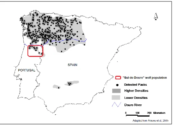
Currently, in Iberian Peninsula, two wolf populations are recognized (Chapron, et al. 2014): i) the NW population, comprising most of the Iberian wolf range and occupying the northwestern part of the peninsula, including the north of the Douro River in Portugal ; ii) another small and isolated population located in Sierra Morena, Southern Spain; although this population is considered on the verge of extinction (Fig. 1) (Blanco and Cortés 2002; López-Bao, et al. 2015). Furthermore, a small section of the NW population located south of the Douro river in central Portugal could be considered as an additional third wolf population due to strong evidences of isolation and differentiation from the remaining Iberian populations (Godinho, et al. 2007; Grilo, et al. 2004).
Figure 1- Wolf distribution and detected packs in Iberian Peninsula, with a red square representing the South Douro river wolf population in Portugal (adapted from Alvares, et al. (2005)
In Portugal, wolf population is currently estimated in 63 packs occupying a distribution area of 13,600km2 in north of Douro river and 6,800km2 in south of this river, which represents only 20% of its original range (Pimenta, et al. 2005). Wolves in Portugal occupy mostly agricultural habitats and live closely to human settlements feeding mostly on livestock, which can constitute up to 80% of their diet due to low numbers of wild ungulates (Petrucci-Fonseca 1990; Vos 2000).Similarly to most of the wolf range, in Portugal wolves were heavily persecuted mainly because of livestock damages and myths against this carnivore (Álvares, 2011). Currently, the wolf is strictly protected in Portugal since 1988 and considered endangered (EN) (Pimenta, et al. 2005), although illegal persecution is still very common (Blanco and Cortés 2002; Grilo, et al. 2004). Furthermore, wolves are also affected by habitat degradation and infrastructure development, especially roads which cause casualties and habitat fragmentation (Álvares, 2004; Pimenta, et al. 2005).
Unlike the rest of Europe, where wolves are showing a positive trend, wolf populations in Portugal are still declining and facing a high risk of extinction, particularly in the south of Douro river (Santos, et al. 2007). In fact, this isolated population is estimated in six packs with low reproductive success comprising a total of approximately 30 individuals (Pimenta, et al. 2005). Direct human persecution is still the main cause of wolf mortality, with almost 50% of known mortality causes
(Alexandre, et al. 2000). Because of its low population size, isolation, high degree of fragmentation, the south of Douro river wolf population is expected to become inbreed and with a reduced genetic diversity, consequently, reducing its potential of adaptation due to higher vulnerability to stochastic environment changes (Hedrick and Kalinowski 2000), increasing its risk of extinction.
Throughout the entire wolf range, other isolated wolf populations have passed through high risk of extinction or effectively have been extinct. The most emblematic case in Europe was the Swedish wolf population that was officially declared as extinct during twenty years, when a new breading pair founded a new population (Liberg, et al. 2005). Today it presents high levels of inbreeding and a reduced genetic diversity. Another emblematic example comes from the Isle Royale, in Lake Superior, USA, an island only occasionally connected to land when an ice bridge forms. Genetic analysis showed that only three individuals founded this population in 1949 or 1950, with the exception of one individual that arrived to the island in 1997 (Peterson and Page 1988). This population shows signs of high inbreeding depression accompanied by high mortality rates, lower number of breeding females and bone malformations (Adams, et al. 2011; Räikkönen, et al. 2009; Wayne, et al. 1991). These two cases show how crucial it is to understand past population histories to understand the present and plan the future. Knowing the genetic history of the wolf population in South Douro River in detail, and knowing there are no previous genetic studies for these populations, will aid in understanding the demographic history and consequently the impacts of inbreeding and small population size in as large carnivore such as wolves.
Objectives
This study aims to evaluate the demographic history of the South Douro river wolf population in Portugal using two different approaches: an assessment of both distribution trends and genetic patterns.
By analyzing historic presence records already available and also, combining the use of modern and historical samples with next-generation sequencing techniques and known SNPs we hope to answer the following questions:
i) which was the extinction rate and level of fragmentation related to the negative distribution trend in this population in the past?; ii) what were the causes that might have influenced the drastic reduction in population size and range?; iii) which were the demographic consequences of this range decline, in terms of effective population size and genetic diversity?; and iv) Is there evidences of a bottleneck in the past and which was its magnitude?.
In particular, the main objectives of this work are:
Assess trends on wolf distribution and fragmentation since the beginning of the 20th century.
Evaluate the probability of wolf persistence along the 20th century
Compare the genetic diversity (e.g. observed heterozygosity) and dissimilarity (e.g. number of private and rare alleles) between contemporary and historical wolf populations.
Estimate the effective population size (Ne) of the two contemporary wolf populations located at North and South Douro river and the effective population size of the historical South Douro wolf population
Understand the demographic history of wolf populations in Portugal and the consequences of their strong range decline.
Materials and Methods
Study area
This study was focused is the entire area of continental Portugal, particularly where the wolf occurred since the beginning of the 20th century. Continental Portugal is located mainly in the Mediterranean biogeographic region, with the exception of northwest, which is included in the Atlantic region (Costa, et al. 1998; ICNB 2010; Pimenta, et al. 2005). Current wolf range in Portugal corresponds to areas of moderate human density with less than 50 inhabitants per km2, with the majority of the areas (60%) accounting less than 25 inhabitants per km2 (Pimenta, et al. 2005). The climate is temperate, with a mean annual temperature ranging from 7ºC to 16ºC, and with an average annual precipitation ranging from 400 mm at the eastern lowlands to 2800 mm in the western mountains (Carmo, et al. 2011). Land cover is dominated by agricultural and agro-forestry areas alternating with mixed forests and shrub patches (Nunes, et al. 2005; Pimenta, et al. 2005). Within current wolf range, wild prey populations are scarce but there is a great availability of livestock, especially in the mountainous areas, which comprises the main food resource for wolves (Álvares 2004; Pimenta, et al. 2005).
Distribution trends
We assembled distribution maps with current and historical records of wolf presence in Portugal. The information for current wolf presence was based in systematic data from the most recent national wolf census, conducted in 2002/2003 and using both confirmed and probable presence detected by field sampling at a 10x10km UTM grid (Pimenta et al., 2005). The historical records were obtained from previous studies assessing the evolution of wolf distribution since 1900. (Fonseca 1990; (Fonseca and Álvares 1997). Historical records from Petrucci-Fonseca (1990) were available for the whole country in 10x10km UTM grid from 1900 to 1990 in a ten years interval, and were obtained from news on local and national journals, official hunting statistics and inquiries to local people (Petrucci-Fonseca (1990). This information was later updated for the more recent decades in the southern half of Portugal (south of Tejo river) by compiling further historical presence records of wolves in a regional literature review and a wide effort of inquiries to local people throughout all potential wolf range (Petrucci-Fonseca and Álvares (1997). Since these distribution maps were only available in paper format they were georeferenced using the software qGIS (QGis 2011) and the information from both bibliographic sources was combined. A database with all historical records of wolf presence at 10x10km UTM
grid was assembled. We used the assumption of past presence for each 10X10km cell when presence was confirmed for a previous decade in the same cell. This strategy counterbalanced the scarcity of data for the first decades (1900 to 1920) and allowed us to produce clearer maps of wolf distribution in the past. Maps were enriched with topography and main rivers, features that can influence the dispersion and presence of wolves. A total of six maps from 1900 to early 2000 were built using the following time periods: 1900/1910; 1920/1930; 1940/1950; 1960/1970; 1980/1990; 2002/2003.
To evaluate whether population isolation occurred in wolves over time, we calculated a buffer area around every of wolf presence (continuous 10x10 km cell with wolf presence) considering the potential of wolf dispersal between areas. Since wolf dispersion patterns can vary we used two different buffers, the first buffer with 30 km radius of dispersion, which is considered an average dispersion, and the second buffer with a 50km dispersion, a more conservative view, considering available information on dispersal distances of Iberian wolves (Álvares 2011; Blanco and Cortés 2007). We then generated those buffers for each time period.
Based in records of wolf presence we calculated several different parameters for both the North and South of the Douro River populations, such as the evolution of range extent and number of population fragments along each time period since 1900. Moreover, by using reference values of current wolf densities we estimated for both areas the total number of wolves potentially in each decade occurring. Reference values for wolf densities were obtained from the last national wolf census in Portugal, considering a conservative value of 2 wolves/100km2 in the North of Douro river population and 1 wolf/100km2 in South Douro river population (Pimenta, et al. 2005).To evaluate the major habitat changes within wolf range along time periods and both in North and South Douro river we used data on official agricultural statistics over the past century previously compiled by Pereira dos Santos (2015), namely the agricultural area occupied by wheat, rye, corn, beans, grain, legumes, potatoes and olive grove (as a measure of refuge availability for wolves) and the number of cows, pigs, sheep and goats (as a measure of food availability for wolves.
To assess the number of population fragments along time periods, we considered that a fragment occurred when it was separated by a distance bigger than 10 km. Next, once we identified population fragments, we calculated the number of wolf population fragments in each decade, their size and their evolution (persistence/extinction) in time looking at the fragment they originated and when they disappeared. In addition, we estimated the number of wolves expected to exist in each
isolated fragment using the same reference values of wolf density described above (Pimenta, et al. 2005). We also accessed the distance between the fragment and the closest wolf population fragment, and the number of fragment in the vicinity. We used this information to estimate the probability of a wolf population fragment to persist over time in relation to different population parameters. To do this, for each fragment in a given decade we related its persistence or extinction to the abovementioned population parameters the decade before, assuming that the observed status in a given decade and fragment will be influenced mainly by the past attributes of such fragment. To conduct this analysis, we tested two non-mutually exclusive hypotheses explaining the probability of persistence of a wolf fragment over time. The first hypothesis predicted that the probability of persistence was higher when the fragment was bigger, and since the fragment area is correlated with the number of wolves (Spearman correlation test p-value=1), a higher number of wolves would also ensure the persistence of the fragment. The predictor used in the model representing the first hypothesis was the area (we did not use the number of wolves because of the high correlation value between the number of wolves and fragment size). The second hypothesis suggested that the fragments would disappear if there was few or far fragments nearby. The predictors used in the model representing the second hypothesis were the number of closest fragments and the distance to the closest fragment. These predictors informed us about the influence on the probability of wolf fragment persistence over time in relation to the wolf population fragmentation processes in the area. Since we had information for the same fragment in several decades, we built Generalized Linear Mixed Models (GLMMs) with Binomial distribution and logit link using the R package “lme4” (Bates, et al. 2014; Bates, et al. 2013) Candidate models (including the null model and the full covariate model) were compared using the sample-size corrected Akaike Information Criterion (AICc). (Burnham & Anderson 2010). We also estimated AIC weights (wi), which indicates the probability that the model selected is the best
among the candidates (Burnham and Anderson 2010). We selected models with ΔAICc < 2. All statistical analyses were performed in R 3.0.2 (R Core Team, 2013).
Molecular patterns
Sample collectionA total of 38 modern wolf samples were collected from dead animals (road kills or hunting) between 2000 and 2014 and comprise 23 animals from the south of Douro population and 15 from the north of Douro population in Portugal (Table 1). All samples were stored at -20ºC. Samples consisted mainly of tissue, like ear tissue, and organs, such as kidneys or heart.
A total of 42 historical samples were collected from skulls, pelts and stuffed specimens and comprise 25 animals from various museums and 17 from private collections (Table 1). It was important to collect as much as possible tissue in each sample for a successful extraction, given the expected low quality and amount of DNA. Historical tissue samples, especially pelts and stuffed specimens in private collections, were collected from tissue near the paw or inside the ear, where human contact was expected to be lower, in order to decrease the risk of exogenous contamination. Both bone and tissue samples were collected with sterilized material and stored in a zip lock plastic bag. These bags were only opened again when performing DNA extraction in the non-invasive laboratory.
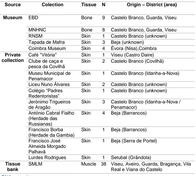
Table 1-Samples used in this study and their origin, location and type. EBD-Estación Biológica de Doñana, MNHNC-Museu Nacional de História Natural e das Ciências, RNSM-Reserva Natural da Serra da Malcata, SMLM- Sistema de monitorização de Lobos Mortos.
Source Colection Tissue N Origin – District (area) Museum EBD Bone 9 Castelo Branco, Guarda, Viseu
MNHNC Bone 8 Castelo Branco, Guarda, Viseu
RNSM Skin 1 Castelo Branco (unknown)
Tapada de Mafra Skin 3 Beja (unknown) Coimbra Museum Skin 4 Évora (Nisa),Coimbra Private
collection
Café "Vitória" Skin 1 Viseu (Castro Daire) Clube de caça e
pesca da Covilhã
Skin 2 Castelo Branco (Covilhã) Museu Municipal de
Penamacor
Skin 1 Castelo Branco (Idanha-a-Nova) Liceu Nuno Álvares Skin 2 Castelo Branco (unknown) Colégio “Padres
Redentoristas”
Skin 1 Castelo Branco (unknown) Jerónimo Trigueiros
de Aragão
Skin 3 Castelo Branco (Idanha-a-Nova / Penamacor)
António Cabral Fialho (Herdade das
Russianas)
Skin 4 Beja (Barrancos)
Francisco Borba (Herdade da Gambia)
Skin 1 Beja (Barrancos) Francisco José
Almeida Morgado Palhavã
Skin 1 Beja (Serra de Portel)
Lurdes Rodrigues Skin 1 Setubal (Grândola) Tissue
bank
SMLM Muscle 38 Viseu, Aveiro, Guarda, Bragança, Vila Real e Viana do Castelo
DNA extraction
Our historic and modern samples could be comprised in four different categories; bone museum samples, tissue museum samples, modern samples never
successfully extracted and modern samples previously extracted and successfully genotyped. For the first three categories extraction followed the Ancient DNA extraction protocol described in Rohland and Hofreiter (2007) and perfected in Dabney, et al. (2013). For samples that had already been successful extracted we used the Blood and Tissue kit from Qiagen.
Ancient DNA extraction protocol
Rohland and Hofreiter (2007) protocol was specifically created to successfully extract ancient DNA from bone samples, and has been used in several studies (Green, et al. 2010; Reich, et al. 2010). Even though this protocol was specifically developed for bone samples, we also applied it in tissue samples with some slight alterations.
Given the origin of the samples, special precautions were taken in account. The DNA extraction took place in a dedicated clean room, where only non-invasive or historical DNA was extracted. This room is equipped with UV lights that sterilize the room and eliminate all present DNA, also, before starting, all the counters were cleaned with bleach and ethanol to further ensure a clean surface. All the buffers were prepared and then placed under UV light. The rest of the material was washed with bleach and UV treated for at least 15 minutes, in order to destroy any contaminant.
Tissue samples were washed with a PBS solution overnight to clean any leftover ethanol, foreign DNA or other contaminating residues. After that, tissue samples were cut in small pieces and bone samples were transformed into a powder with the help of a mortar and a pestle. Samples were then weighted. 50 to 150mg of sample were then placed in a 2.0mL Safelock Eppendorf tube sealed with parafilm and digested overnight at 37ºC in the extraction buffer solution, containing, ultrapure water, 0.5M EDTA, Tween 20 and Proteinase k (New England Biolabs).
A
B
C
D
E
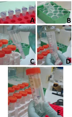
Figure 2-Assembly performed in the extraction protocol A-Labeld MinElute spin columns B- Zymo extension reservoirs C-Assembly of columns and reservoirs D-Assembly inside de 50mL falcon tube. E-Assembly with sample and binding buffer inside.
After digestion, only 11 samples were extracted at a time, to avoid cross-contamination. Also, in each extraction a negative control was used in order to see if there were any contaminants in the buffers. If, after extraction, the negative control presented traces of DNA the whole batch would be discarded and extracted again.
After digestion, a centrifugation was performed and the supernatant transferred to a 50mL falcon tube containing a mixture of binding buffer (ultrapure water, isopropanol, tween 20 and guanidine hydrochloride) and sodium acetate. Because this originated a big volume of liquid, Zymo extension reservoirs were assembled with the MinElute spin column from Qiagen. Then this assembly would be put inside a 50mL falcon tube without the collection tube (Fig. 2). This mixture was then transferred to the assembly, centrifuged, inverted and centrifuged again. With the tissue samples, sometimes extra minutes and/or rotations per minutes were required for all the liquid to pass through the column. Afterwards, the assembly would be taken apart and the column would be put back in the collection tube, the flow through was discarded. After a dry spin, PE buffer (Qiagen) were added and centrifuged, the flow through was discarded. This step was performed twice in order to clean the membrane of the column.
After that, the DNA was eluted twice with 25µL of TET buffer to a 1.5mL Eppendorf Low retention tube, both elutions were kept in the same tube. Since the concentration was low in some samples, given their age or conservation, a second elution with 50µL of TET buffer was performed to a different tube and, when needed, a second extraction was performed to obtain the needed amount of DNA for library preparation (100ng). Extractions were always performed in the presence of blanks to monitor possible contaminations.
Blood and Tissue Extraction kit
For modern, good quality samples the DNeasy Blood & Tissue kit from Qiagen was used, and three replicates of each sample were performed in order to obtain a good amount of DNA.
Since samples were stored in ethanol they were washed in PBS to clean any leftover residues. About 25mg of tissue was used. The DNA was eluted twice with 200µL of AE buffer and elutions were kept separate.
DNA Quantification
Two DNA quantification methods were used to measure concentration of both modern and historical samples, the Qubit and the Picogreen. These methods are based in the same principle, a fluorescent dye ligates to double stranded DNA and
emits fluorescence which is then captured by a lens. According to the standards concentration, a calibration curve is obtained and the concentration for each sample calculated. Qubit was used with two DNA standard concentrations and Picogreen with eight standards.
Qubit quantification was performed with the High sensitivity kit that can detect DNA from 0.2 to 100ng, the quantity range we expect our DNA to have. A new calibration to the Qubit machine was done to assure accurate reads, and each sample was read at least two times to obtain the most correct concentration. If there was disparities between reads, a third read was performed.
Picogreen was used with the standard scale that measured values between 0 to 100ng/µL and three reads were made for each sample.
The values obtained by both methods were compared and in the case of some disparities, a new reading using Picogreen was performed and then the outlier number was discarded. The final concentration for each sample was obtained by averaging between the two different quantification methods.
When needed, samples were concentrated in a Speedyvac. To avoid contamination, the Speedyvac was taken inside the clean room and cleaned with bleach and UV treated. To avoid cross contamination a two space interval was left between samples. Each sample was concentrated until no liquid was visible. After that, to all of the concentrated samples 21µL of clean deionized water were added, the samples were then left in the fridge overnight to elute the DNA from the pellet, before they were stored at -20ºC.
EzRAD for SNPs discovery
Choosing the restriction enzymes
One of the most crucial steps in a RADseq protocol is choosing the restriction enzymes, because different enzymes cut at different sites and will originate different size fragments. We used two different approaches to choose the restriction enzyme, i) in silico tests using SimRAD (Lepais and Weir 2014), an R package and ii) digestion tests with some samples.
SimRAD is a package for R that allows to simulate an in silico digestion with a plethora of restriction enzymes. This program allows for the researcher to include a portion of the genome of their species or, if not available, a related one, and simulate the number of fragments expected when cutting with one or more restriction enzymes. In our study we choose several restriction enzymes to simulate with, like the ones
mostly used in RADseq protocols (Davey and Blaxter 2010; Kai, et al. 2014) and the ones that most frequently cut on the dog genome, namely, SbfI, BamHI-HF, MspI, PstI, BclI, BglII, Sau3AI, RsaI, HoeIII, EcoRV, SspI, MboI and AluI (Paxinos, et al. 1997). We tested enzymes both alone and in double digestions. For the simulation, we used a quarter of the dog genome, given that the wolf genome is not yet available. We then estimated the number of originated fragments and the number of fragments obtained with the size between 100-150 and 210-260. After all the simulations we concluded that the best enzymes were Sau3AI, MboI and AluI.
We then proceeded to the digestion for some of our samples with these enzymes in order to choose the best combination. We tested a double digestion with MboI and Sau3A1 as described in the EzRAD protocol (Toonen, et al. 2013), and a digestion with AluI. We also tested the optimum amount of enzyme, 0.1 µL or 0.2 µL per sample, and the optimum amount of digestion time, 8, 4, 3 and 1 hour.
Library preparation
We choose to perform the EzRAD protocol with some modifications because of its simplicity. We selected the Ilumina Nano kit because it allowed samples to have only 100ng of DNA, a very useful characteristic given the origin of our samples.
We performed DNA digestion in all of our samples. Then we set a thermocycler with the following program: 37ºC for 8 hours followed by 20 minutes at 65ºC for thermal inactivation and then hold at 15ºC. After digestion, a bead clean up with a proportion of 1 to 1.8 was performed in order to eliminate fragments smaller than 100bp, it is crucial that the beads (Illumina) are thoroughly vortexed in order to be dispersed in the solution. Afterwards each sample was eluted in Resuspension buffer (RSB) also provided by Illumina. The following steps are the same as the ones performed in Illumina’s TrueSeq Nano protocol, with only slight modifications. We followed the LS protocol (Low-sample) and only did 24 samples at a time, in order to avoid mistakes. We had to repeat each step 4 times in order to make an entire plate of 96 wells. Two end-repair were performed and the DNA was resuspended in RSB. Then A-Tailing was performed and each sample was ligated to a different adaptor. This allows us to distinguish each sample once they are pooled. We used the DAP plate (Illumina) in order to have 96 different adaptors. This was followed by two consecutive beads clean up with a proportion of 1 to 1. The DNA was eluted in RSB and transferred to a new plate.
In order to size select the fragments and eliminate unligated adaptors, we ran our libraries in a 2% ultra-pure agarose gel (Bio-RAD), this helped visualizing the
amount of DNA we had in each sample and see the distribution of the fragments resulting from the digestion. The agarose gel ran in a 1x TAE solution (Tris, acetic acid, EDTA). The 2% agarose gel was prepared with 3g of ultra-pure agarose (NzTech), 150mL of TAE and 15µL of Sybr Gold (Life technologies). The melted agarose was poured in a 12x14cm tray and let set for at least half an hour. Each comb had 14 spaces so each gel allowed us to run 5 samples at a time while leaving a gap between them in order to avoid cross-contamination, and using two ladders in the extremities (Fig. 3). With these configurations a total of 20 gels were done.
For the sample preparation we used 20µL of DNA plus 4µL of Blue/Orange loading dye (x6) (Promega). For the ladders we used 17µL of RSB, 4µL loading dye and 3µL of HyperLadder 4 100bp (BioLine). The gel ran at 120V for 120 minutes or until the ladder fully separated.
The gel was then visualized using a UV transluminator (BioRAD) and a band between 300 and 500bp was excised. This size already includes the ligated adaptors, so our target DNA should had a length between 380 and 180bp, since the adaptor size is 120bp. Between each sample a different scalpel was used in order to avoid cross-contamination, and between gels the transluminator was cleaned with bleach and ethanol. A picture of each gel was taken before and after the cut. The excised agarose was then divided in two 2mL Eppendorf tubes with its weight not exceeding 400mg.
Figure 3- Sample order in agarose gel. Each gel had two ladders in the extremities and five samples, always separated by one well to avoid cross-contamination.
The extraction of the DNA from the agarose gel followed the Qiagen PCR purification kit with some slight alterations. To each tube the triple the amount of weigh was added in QG buffer. Each tube was vortexed briefly and let the agarose dissolve for at least ten minutes at room temperature. Next the same volume of the weight in isopropanol was added to each tube inverted. MinElute columns were assembled in the collection tubes provided by Qiagen, the amount of columns needed is the same as Eppendorfs, usually two per sample.
A volume of 700µL of the mixture for each column were transferred to its respective column and centrifuged, the flow through was discarded. Depending on the weight of the sample this process was repeated until there was no more liquid left. Then QG buffer was added to each column and again spun down, the flow through was
discarded. PE buffer was added to each column and once again the samples were centrifuged and the flow through discarded. The discard any residual ethanol we repeated the centrifugation for an additional 3 minutes. We then put the column in a new 1.5mL Eppendorf tube and added Elution Buffer and waited 2 minutes, then centrifuged. Since we had two columns per sample we polled both elutions in the same tube, leaving us the 24µL of clean size-selected DNA.
In the enrichment faze, only 20µL were needed but, since not always all the liquid is recuperated, an extra 4µL are eluted, also this extra amount can be used for testing the quantity and quality of DNA we had before the PCR enrichment.
Library enrichment
In this step our libraries were enriched using PCR with primers designed to complement the adaptors, so, only fragments which had both adaptors ligated were amplified. This reaction used a PCR primer cocktail (Illumina) and an enhanced PCR Mix (Illumina) both provided in the TrueSeq Nano.
We used the PCR program advised by Illumina with 5 additional cycles. The DNA was the eluted RSB and transferred to the final plate. 2µL were tested in a 2% agarose gel to visualize the final library.
Validate library using qPCR
To validate the library and know the quantity of DNA to be used for each sample in the final pool, all samples were quantified using qPCR with the Kappa protocol.
For each samples, two dilutions were performed, 1:40000 and 1:100000. For each of those dilutions two replicates were done. The standards used had a 1:10 dilution between them with the lower standard having a concentration of 2x10⁻³, Replicates were checked for deviations and outliers were discarded.
Illumina HiSeq Run and data analysis
The 96 samples were normalized at 10nM and evenly pooled. After pooling two successive dilutions were done to 2nM and 20pM. The samples then ran a rapid run at 11.5pM in two lanes with paired-end reads of 150 cycles in the HiSeq 1500 sequencer. Illumina cluster density and QC scores were observed in order to assure the quality of the run.
The first step for analysis procedures of the reads from the Illumina run is demultiplexing, which was performed using the command process_radtags from STACKs (Catchen, et al. 2011). After this, reads from the same sample run on lane 1 and 2 were merged, using the command cat from the command line.
Since most of the samples were from museums we should expect contamination, and non-wolf reads were discarded through alignment to the dog reference genome. For that, every chromosome was download from ensembl.org (Flicek, et al. 2013) and concatenated (with the command cat) to create a sequence containing the entire dog genome. The reference genome was indexed to decrease computer power needed on alignments. For the indexing we used bowtie2 (Langmead and Salzberg 2012) with the command build. Bowtie2 was also used for alignments. This alignments enable to check the percentage of reads that aligned to the dog reference genome. With this alignment we performed an ANOVA and a t-test to analyze possible significant differences in correct amplification related to the age of samples and also their type (tissue or bone).
The total reads that mapped to the dog genome were extracted in a separate file to continue with the analysis.
Two different runs were performed in stacks, one creating an artificial reference genome with reads obtained in the run, and a second one using a reference genome, in this case the dog genome, to do the SNP calling.
Genotyping previously known SNPS
An alternative method to SNP discovery is genotyping already known SNPs. We selected randomly a total of 224 SNPs known previously to be polymorphic in the Iberian wolf population (vonHoldt 2010). These SNPs were genotyped in a SNP genotyping platform at the Instituto Gulbenkian de Ciência (IGC), Portugal. Two of the samples were sent in duplicate, one from a museum sample and one from a tissue sample.
The resulting database was analyzed in order to remove monomorphic loci and individuals with missing data higher than 75%. The final database comprised 58 individuals, 33 known wolves, 6 known dogs and 19 historical samples that were considered wolves on collections. To test the origin of these historical samples an assignment analysis was performed using the software Structure (Pritchard, et al. 2000). Structure was run using the admixture model and correlated allele frequencies, with 104 burnin and 105 MCMC iterations, using popflag for known wolves and dogs. 4 dogs were removed from the database.
Samples were grouped in four sets, i) historical samples (N=15, from 1950-1990), ii) modern south of Douro samples (N=15), iii) modern north of Douro samples (N=17) and iv) dogs (N=10). Dogs that were identified in the previous assignment
analysis were included in dog population. Population genetic parameters such as observed and expected heterozygosity, the number of private alleles and of rare alleles were calculated using GenAlEx (Peakall and Smouse 2012, 2006). Each individual was treated as a population to obtain individual measurements. Results were plotted in graphs showing the evolution of these parameters through time.
Wolf samples were used to estimate the effective population size using NeEstimator (Do, et al. 2014). This program allows to estimate effective population size (Ne) using several different methods: Linkage Disequilibrium (Waples and Do 2008), Heterozygosity excess (Zhdanova and Pudovkin 2008), Molecular coancestry (Nomura 2008) and the temporal method (Jorde and Ryman 2007; Nei and Tajima 1981; Pollak 1983; Waples 1989). We opted to use the linkage disequilibrium method with monogamy mating to calculate the effective population size for the historical, modern south and north of Douro populations because it is known to perform better for the quantity and quality of data that we have (Do, et al. 2014).
Structure was used a second time to cluster individuals in putative populations. Structure was run with 254 burnin and 55 MCMC iterations. Used 3 iterations with K going from 1 to 6. Number of most probable clusters were calculated using Structure Harvester. We them plotted these results geographically using qGIS using the know location of each sample.
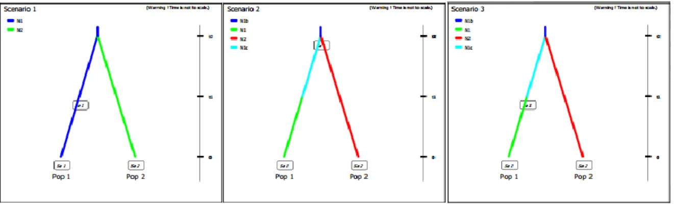
We also tried to evaluate the population history using an ABC method with the DIYABC (Cornuet, et al. 2014), we assumed two populations that diverged in the past, one (South Douro) suffered bottleneck and the other maintained its size. The priors assumed were: Merged populations with a size between 15 and 250 wolves, historical population with 15 to 250 wolves, current south Douro population with 15 to 70 wolves and current north Douro population with 15 to 250 wolves. The divergence time was between 50 to 200 years ago and the bottleneck occurred between 10 to 50 years ago (Fig. 4).
Figure 4-Models tested in DIYABC. The first model is the null hypothesis, the second one suggests that historical samples were taken before the bottleneck that occurred in the South of Douro population, and the third model assumes historical samples were taken while the bottleneck was occurring. We assumed that the North of Douro population maintained its size.
Results
Distribution trends
Range patterns, fragmentation and estimate population size
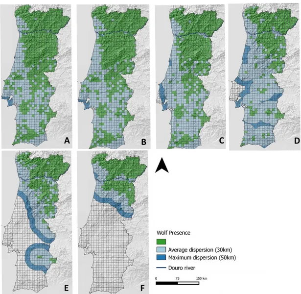
The compilation of presence records showed the rapid decline in the Portuguese wolf population during the twentieth century (Fig 5). In the beginning of the last century, the wolf population covered almost all national territory (56,600km2) while currently wolves only occur in 19,500km2, corresponding to 34.5% of the distribution area in 1910 (Fig 5). Considering the wolf range only located South of Douro river, the decrease in range extension size is even more pronounced, decreasing to only 11% of the distribution area in 1910, emerging small and isolated fragments over time, a pattern that was not observed in the Northern region of the country, where wolves persisted and still maintain 89% of the distribution area in 1900.
Considering the two buffers that represent potential dispersion distances, one population isolate emerge in the decade of 1980-1990 with the 50km buffer. Two isolates emerged, one in the 1960-1970 and another in 1980-1990, considering the 30km buffer.
Figure 5-Wolf distribution between 1900 and 2003 represented in 10x10km squares. Level of fragmentation considering two different buffers of wolf dispersion distances, a 30km buffer (light blue) and a 50km buffer (dark blue).
For wolf presence isolates considering a distance bigger than 10Km, their number increased over time and the two areas of the Portuguese wolf population showed different patterns. The North Douro river population maintained a continuity throughout the 20th century, while the southern population had an increasing number of fragments until the decade of 1960-1970 when it reached the maximum of 16 fragments, and then a decline till the present situation with only one fragment left (Fig. 6 and 7). As expected, the estimated number of wolves followed the decrease in the range size, however, as observed in the regression line for the south population (Fig. 8), this decrease was not steady. Between the decades of 1900 to 1910 the population lost only 1% of its range and between 1930 and 1940 lost 12%. One of the biggest decreases in population size was between 1950 and 1960 where the population lost