____________________________________________________________________
Mergers and Acquisitions:
The case of United and Continental
Airlines
Jorge Miguel Braga Ferreira
(152412043)
Advisor: Peter Tsvetkov
Dissertation submitted in partial fulfillment of requirements for the degree
of MSc. in Finance at Universidade Católica Portuguesa
Abstract
The US airline industry is characterized to be an industry with a high competition mainly in the domestic segment. In order to face this competition several airlines entered in mergers and acquisitions (M&A) deals as way to consolidate its position in the market. This trend was accentuated with the global recession that brought several challenges to this industry. For this reason, the merger between United and Continental Airlines, two major US carriers, are being planned and its valuation and analysis are the focus of the present dissertation. By taking in account the current conditions of both airlines are estimated potential synergies of around 37,4% of the merged airline’ equity value without synergies which represent 69% of the current Continental’s market capitalization, the airline seen as the target. Given this, it is suggested an offer with a premium of 21,6% over the current Continental’s market capitalization which will constitute a deal of $3,018 million, which is here suggested to be paid all in stock.
Acknowledgments
The author would like to acknowledge to his advisor: Peter Tsvetkov by his availability and feedback provided which were crucial for the development of the present dissertation. Also he would like to express his acknowledge to his family by their supporting provided during the last months.
List of Contents
1. Introduction ... 10
2. Literature Review ... 11
2.1.Valuation Approaches ... 11
2.1.1. Discounted Cash Flow approach (DCF) ... 12
2.1.1.1.Cost of Capital ... 13
2.1.1.1.1. Risk-free rate (𝑅𝑓) ... 14
2.1.1.1.2. Beta (β) ... 15
2.1.1.1.3. Market risk premium (𝑅𝑚− 𝑅𝑓)... 16
2.1.1.2.The Free Cash Flow to the Firm (FCFF) ... 17
2.1.1.2.1. Terminal Value ... 18
2.1.1.2.1.1. Long-term growth rate ... 18
2.1.1.3.The Adjusted Present Value (APV) ... 19
2.1.2. Multiples valuation approach ... 20
2.1.2.1.Transaction multiples ... 22
2.2.Mergers and Acquisitions (M&A) ... 23
2.2.1. Types of M&A ... 23
2.2.2. Reasons for M&A ... 25
2.2.3. Synergy and the acquisition premium ... 27
2.2.4. Methods of payment ... 29
2.2.5. Post M&A returns ... 30
2.3. Conclusions ... 32
3. Industry and firms analysis ... 32
3.1.Analysis of US airline industry ... 32
3.1.1. Industry overview ... 34
3.1.3. Recent trends ... 37
3.1.4. General growth perspectives ... 38
3.1.5. M&A trends in the industry ... 39
3.2.Firms analysis ... 39
3.2.1. United Airlines... 39
3.2.1.1.Firm overview ... 40
3.2.1.2.Operating revenues and expenses ... 42
3.2.1.3.Profitability ... 42
3.2.1.4.Liquidity ... 43
3.2.1.5.Assets and equity ... 44
3.2.1.6.Debt ... 45
3.2.1.7.Capital expenditures ... 45
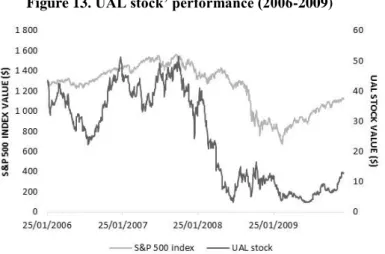
3.2.1.8.Stock performance ... 46
3.2.2. Continental Airlines ... 46
3.2.2.1.Firm overview ... 47
3.2.2.2.Operating revenues and expenses ... 48
3.2.2.3.Profitability ... 49
3.2.2.4.Liquidity ... 50
3.2.2.5.Assets and equity ... 51
3.2.2.6.Debt ... 51
3.2.2.7.Capital expenditures ... 52
3.2.2.8.Stock performance ... 53
4. Firm’s valuation as standalone ... 54
4.1.Operating revenues... 54
4.2.Operating expenses ... 56
4.3.Capital expenditures and depreciations ... 58
4.5.Valuation output ... 59
4.5.1. Free Cash Flow to the Firm (FCFF) ... 59
4.5.2. Adjusted Present Value (APV) ... 61
4.5.3. Multiple valuation ... 62
4.5.4. Sensitivity analysis ... 63
4.5.5. Conclusions ... 65
5. Valuation of the Merged Firm ... 66
5.1.Valuation of the merged firm without synergies... 66
5.2. Synergies estimation ... 67
5.2.1. Revenues enhancements synergies ... 67
5.2.2. Cost saving synergies ... 69
5.2.3. Capital expenditures synergies ... 70
5.2.4. Financial synergies ... 71
5.2.5. Restructuring costs... 72
5.3.Valuation of the merged firm with synergies ... 73
5.4.Breakdown and analysis of the synergies value ... 74
6. Acquisition Process ... 75
6.1.Synergies benefits distribution ... 76
6.2.Estimation of the premium to be offered ... 76
6.3.Method of payment ... 77
6.4.The merger proposal ... 78
6.5.Industry regulation issues and related risks ... 78
7. Conclusion ... 80
8. Appendixes ... 81
List of Appendixes
Appendix 1. Classification of the airlines according with US DOT ... 81
Appendix 2. US major airlines in 2009 ... 81
Appendix 3. Top ten airlines in terms of market capitalization-2009 ... 82
Appendix 4. Top ten airlines in terms of international destiny passengers transported-2009 ... 82
Appendix 5: Top airlines in terms of RPMs and ASMs-2009 ... 83
Appendix 6: Top passengers airlines in terms of RTMs-2009 ... 83
Appendix 7: Top passengers airlines in terms of Operating Profit-2009 ... 83
Appendix 8: Evolution of the annual U.S domestic average itinerary fare ... 84
Appendix 9: Evolution of the total passenger transported in U.S airline industry (2003-2009) ... 84
Appendix 10: Evolution of RPM’s and ASM’s of the US airline industry (2004-2009) ... 85
Appendix 11: Evolution of the fuel price per gallon ... 85
Appendix 12: Evolution of the operating profit/loss and the net income of the US airline industry (2004-2009) ... 85
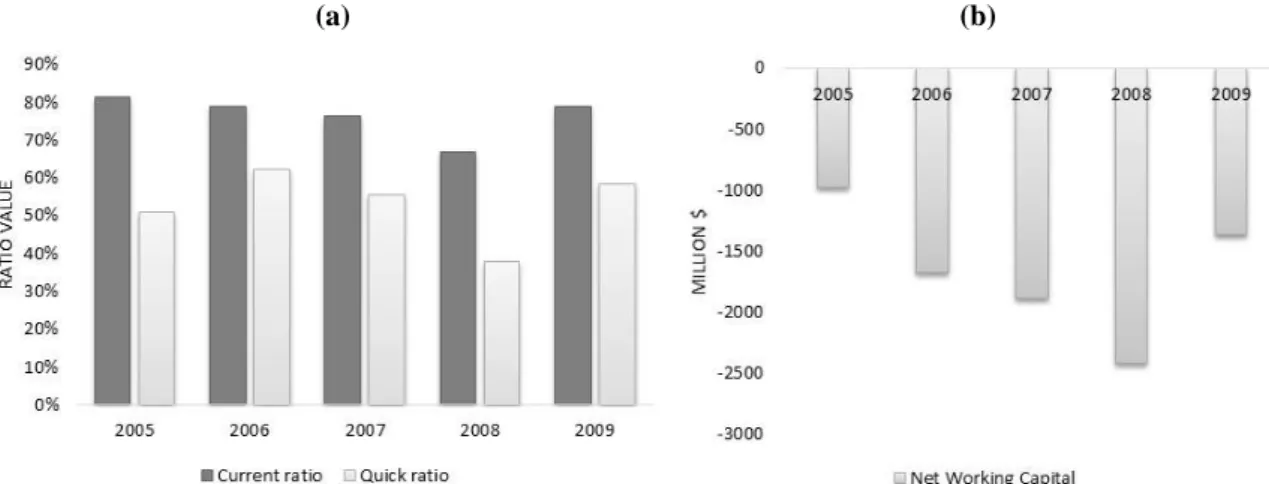
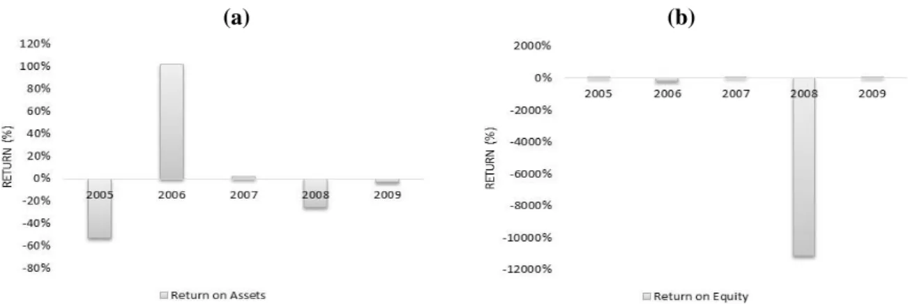
Appendix 13. Evolution of US airline industry ‘current and quick ratios (2005-2006) 86 Appendix 14. Evolution of US airline industry’s return on assets and return on equity (2005-2006) ... 86
Appendix 15. Evolution of US airline industry’s debt ratio and debt-to-equity ratio (2005-2006) ... 86
Appendix 16. Evolution of the number of passengers transported by United (2005-2009) ... 87
Appendix 17. Evolution of the United’s RPM and ASM (2005-2009) ... 87
Appendix 18. Growth rates of the main components of United’s operating revenues .. 87
Appendix 19. Growth rates of the main components of United’s operating expenses.. 88
Appendix 21. Evolution of the number of passengers transported by Continental
(2005-2009) ... 88
Appendix 22. Evolution of the Continental’s RPM and ASM (2005-2009) ... 89
Appendix 23. Growth rates of Continental’s operating revenues... 89
Appendix 24. Growth rates of the main components of Continental’s operating expenses ... 89
Appendix 25. Continental’ average price per gallon of fuel jet (2005-2006) ... 90
Appendix 26. Evolution of Continental’s capital expenditures components (2005-2006) ... 90
Appendix 27. FED US growth predictions ... 90
Appendix 28. GDP growth predictions... 90
Appendix 29. Revenues growth assumptions ... 91
Appendix 30. Historical and Forecasted Balance Sheet of United Airlines ... 91
Appendix 31. Estimation of NWC and short-term investments of United Airlines ... 92
Appendix 32. Estimation of CAPEX and depreciation of United Airlines ... 92
Appendix 33. Estimation of tax rate of United Airlines ... 92
Appendix 34. United’s Debt summary ... 92
Appendix 35. Historical and Forecasted Income Statement of United Airlines ... 93
Appendix 36. Estimation of some of the United’s operating expenses ... 94
Appendix 37. United’s FCFF approach ... 95
Appendix 38. United’s APV approach ... 95
Appendix 39. Historical and Forecasted Balance Sheet of Continental Airlines ... 96
Appendix 40. Estimation of the NWC and short-term investments of Continental ... 97
Appendix 41. Estimation of Capex and depreciation of Continental Airlines ... 97
Appendix 42. Estimation of the tax rate of the Continental Airlines ... 97
Appendix 43. Continental’s debt summary ... 98
Appendix 45. Estimation of some of the Continental’s operating expenses ... 99
Appendix 46. Continental’s FCFF approach ... 100
Appendix 47. Continental’s APV approach ... 100
Appendix 48. Historical and Forecasted Balance Sheet of the merged airline without synergies ... 101
Appendix 49. NWC, CAPEX and Depreciation of the airline merged without synergies ... 101
Appendix 50. Historical and Forecasted Income Statement of airline merged without synergie ... 102
Appendix 51. Merged airline without synergies - FCFF approach ... 102
Appendix 52. Merged airline without synergies - APV approach ... 103
Appendix 53. Localization of exclusive United and Continental’ served airports ... 103
Appendix 54. Aircraft fleet before and after the merger ... 104
Appendix 55. Historical and Forecasted Balance Sheet of the merged airline with synergies ... 104
Appendix 56. Merged airline with synergies debt’ summary ... 105
Appendix 57. Historical and Forecasted Income Statement of the merged airline with synergies ... 105
Appendix 58. Merged airline with synergies - FCFF approach ... 106
1. Introduction
The present dissertation has as main objective to analyze a merger and acquisition (M&A) deal by presenting the strategic and financial reasons to engage in and the possible synergies arise from it. In order to conduct this analysis is presented a real case, the merger between the United and Continental Airlines which announced their merger in 2010.
The period between 2008 and 2009 were characterized to be a period of hard economic conditions derived from the global recession which affect severely all the industries and put in risk the survival of several firms. The airline industry, as cyclical industry, was not exception by which was visible an increase in the debate about M&A’s deals as way to increase the profitability and sustainability at long-term in this industry. Before that is analyzed the above mentioned real case in order to evaluate the possible benefits that can arise from the deal and if it is actually a way to increase their profitability. Firstly, in the literature review are given a theoretical context about the main methods used in firm valuation as well as the main aspects related with the M&A deals which are referred and used in the practical part of the dissertation.
In the next section, the section 3, is presented an analysis of the US airline industry to contextualize and explain the environment which both airlines faced at the time as well as the visible trends stated in the last years. In this section is also analyzed each of one of the airlines in order to provide a portrait of the firms situation and their recent trends.
In section 4 is presented the valuation of each airlines as standalone with the explanation of the assumptions taken and the results achieved. After the valuation of the airlines in an independent way, the section 4 presents the valuation of both airlines together however, without taking in consideration the possible synergies that can arise from the deal. These synergies are approached in section 5 in which is analyzed their possible sources as well as the valuation of the merged airline with the synergies estimated.
Finally, the section 6 approaches the main issues related with the M&A transaction being presented the conclusions of the present dissertation in section 7.
2. Literature Review
The M&A’s are an important component of an economy being a way to increase the effectiveness and the profitability of the evolved firms and the same time solve problems such as the excess capacity of the industry (Koller et al. 2010).
However, the M&A environment is highly changeable and complex where transactions involve a considerable amount of money (Bruner 2004). Several M&A’s transactions fail being the most common reason the fact of the acquirer firm has overpaid the target one. For these reasons, the valuation assumes a central role in this context since is crucial to calculate the value of the target firm as well as the value of the expected benefits in a feasible way (Petitt and Ferris 2013).
Therefore, in order to provide a framework of the M&A’s transactions, this section contains a literature review of the main firm valuation approaches and of the main issues related with the M&A’s.
2.1. Valuation Approaches
According with Koller et al. (2010) the value is ‘the defining of measurement in a market economy’ being a useful measure of performance since it takes in account not only the long-term interests of the shareholders but also of the stakeholders. Therefore, the valuation is assumed as one of the key business skills in order to face business dilemmas by providing information to the managers (Bruner 2004).
The process of choice of the appropriated valuation ‘approach is not straightforward being susceptible to several factors such as the objectives of the valuation, the characteristics of the firm or the preference of the analyst that are performing the valuation (Petitt and Ferris 2013).
Damodaran (2006) refers that there are four major approaches to valuate a firm. The first approach is the discounted cash flow (DCF) which is based in the present value of the expected cash flows generated by the firm. The second approach, the liquidation and accounting valuation, is based on the value of the present firm’s assets. The third, called of multiple or relative valuation, values the firm by the use of multiples of comparable’ firms. Finally, the last approach is the contingent claim/option valuation that conducts the valuation through the use of option pricing models.
None of the methods are seen as the right, in the absolute sense, for valuate a firm since there is uncertainty about the future in each of the values projected (Chaplinsky et al. 2000). Besides that, the numerous of events that occurred in last decades had influence in the validity of the methods and the assumptions that they are based on (Torrez et al. 2006). However, despite these facts, the DCF and the multiples approaches are the most popular and widely used methods among the analysts (Bancel and Mittoo 2014). Thus, in order to provide a more deep understanding, is analyzed these two approaches in the following sections.
2.1.1. Discounted Cash Flow approach (DCF)
According with Steiger (2008) the DCF method is based on a set of predictions about the future of the firm’s business activity being a method that relies on forward looking data. In this line, the author state that the firm’s value is based on the net present value (NPV) of its future free cash flows (FCF) discounted by a discount rate (r):
𝑁𝑃𝑉 = ∑ 𝐹𝐶𝐹𝑡 (1 + 𝑟)𝑡 𝑛
𝑡=0
The FCF corresponds to the amount of cash that is not required for operations or reinvestment activities (Brealey et al. 2006). Concerning to the discount rate, the weighted average of cost of capital (WACC) is indicated as the appropriated one to determine the NPV (Chaplinsky et al. 2000) being their use a consensus point in the finance literature. The WACC will be deeply analyzed in the next section.
This method is one of the most used among the analysts as were shown in different surveys such as the ones conducted by Schall et al. (1978) and Stanley and Block (1984). According with Koller et al. (2010) the popularity of this method is related with the fact that it bases exclusively on the flow of cash in and out of the firm and not on accounting-based earnings. However, there is some reluctance about their feasibility which arises mainly from the uncertainty related with the projections of growth in revenue and earnings that are required (Feldman 2005). For its turn Kaplan (1986) states that the limitations of the DCF method are in fact limitations of the user and not of the technique. Actually, in a study conducted by Kaplan and Ruback (1996) they concluded that the estimations obtained by the DCF method are more close to the actual values than the multiples one thus demonstrating a better performance of this method.
2.1.1.1. Cost of Capital
According with Pratt and Grabowski (2008) the cost of capital is “the expected rate of return that the market participants require in order to attract funds to a particular investment”. It also can be seen, in economic terms, as the opportunity cost of an investor, their required rate of return on assets of similar risk (Bruner 2004). So, the cost of capital represents the cost of firm’s financing in order to pursue their activity that can be a variety of sources since equity to debt passing from several instruments that are available to firms as ways to financing (Modigliani and Miller 1958).
The finance literature states that the firm’s cash flows should be discounted at a rate that represents the firm’s risk characteristics. As the firm’s capital structure consists in equity and debt, the most common and more appropriated rate to use is the WACC which is a rate that takes in account the proportion of each of type of financing after tax cost of capital used (Mitra 2011). The WACC is calculated from the following formula (assuming only two kinds of financing: equity and debt):
𝑊𝐴𝐶𝐶 = 𝐷
𝑉𝑘𝑑(1 − 𝑇𝑚 ) + 𝐸 𝑉𝑘𝑒
Where 𝑘𝑑 is the cost of debt, 𝑘𝑒 the cost of equity, 𝑇𝑚 is the marginal tax rate and 𝐷
𝑉 and 𝐸
𝑉 represents the ratio of each source of finance in the total value of the firm. In this
line Fernández (2011) states that the WACC is an weighted average of two significant components: a cost that is from debt and an required return, more specificlly the required return to equity, that according with the author is not a cost.
In general the finance literature states that to calculate the WACC should be used the target market weights of both sources of financing instead of current book weights in order to reflect the current conditions of the market. When the management repay the debt and if not want to change the capital structure it will repurchases shares and this must to do in market values. Other aspect is that the current weights may not represent the normal observable capital structure and so must be used the target weights that will prevail in the future (Koller et. al 2010 and Bruner 2004).
In terms of the cost of debt (𝑘𝑑 ) it is calculated after taxes to reflect the benefits of the tax deductibility of the interest (Brotherson et. al 2013). In its calcultion is commonly used the promised yield on newly issued debt of a firm (Erhardt 1994),
however, Cooper and Davydenko (2001) state that this way is not correct being necessary a measure that reflects the probability of default. According with Pratt and Grabowski (2008) in certain situations the rate that the firm pays is not the current rate of the market and not reflects the current conditions of the firm, only reflecting the conditions of the time in which was issued. So, to take in account the current conditions of the firm, the analyst can use the debt ‘firm rating and infer from it the level of interest that the firm will pay according with their condition.
In its turn, the cost of equity (𝐾𝑒) is commonly calculated through the Capital Asset Pricing Model (CAPM) which is given by the following formula:
𝐾𝑒 = 𝑅𝑓+ 𝛽(𝑅𝑚− 𝑅𝑓)
According with Bruner (2004) this method is the most appropriated since it focus explicitly in the risk-return relationship however, Koller et. al (2010) states that this method no provide enough guidelines to use in firm valuation namely in the estimation of each of its components. Despite the criticism about their use, the CAPM keeps as the most popular method as can be seen in the survey conducted by Welch (2007) in which 75% of finance professors recommend the use of this method to calculate the cost of equity. In the following subsections the author analyzes in more detail each component of the CAPM.
2.1.1.1.1. Risk-free rate (𝑹𝒇)
The risk-free rate is the first component of the CAPM model and according with Férnandez (2004) it is the rate that is obtained from the acquisition of governments bonds at the date of the estimation of the cost of equity.
Koller et. al (2010) state that in order to calculate in a consisiting way the cost of equity and consequently the cost of capital should be use a government bond with a maturity equal to the time that is expected that cash-flows will be generated. However, the authors mentioned that the analysts frequently choose for simplicity the 10-year government bonds as proxy in the case of U.S. In other hand, Mukherji (2011) conducted a empirical study in order to analyse the best proxy for the risk-free rate in the U.S market and concluded that the Treasury bills are the best proxies to this rate than the long-term government bonds at any investment horizon since they have less market and inflation risk exposure.
Beside the importance of the choice of the type of security to use as proxy for the free rate, Damodaran (2008) states that it is also equal important the use of a risk-free rate denominated in the same currency of the cash-flows estimated in order to achieve an accurate result.
2.1.1.1.2. Beta (β)
The other component of CAPM is the beta which is a parameter that measures how much the stock moves face to changes in the market (Koller et. al 2010).
In the finance literature is evidenced that the beta estimation for an individual firm is not the most adequate practice since contains some statistical noise. In order to surpass this problem the analysts estimate the betas for a set of comparables of the firm valuated that operate in same business (Kaplan and Peterson 1998). According with Koller et al. (2010) this practice is better since as the estimated errors are not correlated across the firms, the possible misleading valuations of individual firms tend to be cancel when calculated an average of the industry beta. For this it is need to exclude the leverage effect in order to only compare the operating risks that the firms are facing. This fact lead us to the use of the unlevered beta (or asset beta) which relationship with the leverege beta is given by the follow equation:
𝛽𝑙= 𝛽𝑢(1 + (1 − 𝑡)
𝐷 𝐸)
Where 𝛽𝑙 is the leverege beta, 𝛽𝑢 is the unleverege beta, t is the marginal tax rate
and 𝐷
𝐸 is the debt-to-equity ratio. After this process the unleverege beta needs to be
adjusted to the current capital structure of the firm which will give the appropriated leverege beta. In the same way, Welch (2014) purpose the use of the unleverege beta of the firm valuated at the first stage in order to not introduce misleadings in the results arised from the kind of financing use in the different firms of the industry. The author also states that the use of betas of the industry is valuable mainly in situations in which the firm is private and their investors are well diversified.
In its turn, Kaplan and Peterson (1998) highlight that usually the analysts exclude the conglomerate firms from the estimation of the industry betas but these firms in some cases represent a significant share of the market which exclude them can introduce bias in the beta estimated due the negative correlation between the market capitalization and
betas. According with Berk (1995) this relationship comes from the fact that the firms with a higher risk have a smaller market capitalization due the additional risk premium incorporate in the discount rate of them. The beta, that measures the systematic risk, will be higher for the firms that have a smaller market capitalization misleading the beta’ industry estimation. In order to solve this aspect, Kaplan and Peterson (1998) purpose a calculation of a market-capitalization-weighted industry beta that is achieved by a cross-sectional regression of the individual betas against the industry percentages, which take in consideration the share of their sales that is attributable to the industry.
2.1.1.1.3. Market risk premium (𝑹𝒎− 𝑹𝒇)
The last component of the CAPM is the market risk premium that is the difference between the expected market return and the risk-free rate, or in more secific words, it is the expected rate of return that a risky project should be offer in excess of which the risk-free projects are offering (Welch 2014).
Brealey et. al (2001) state that the average market risk premium over the last 73 years is around 9 percent a year but in other hand Ibbotson and Chen (2003) for the same period estimate a market risk premium about of 5,9% . This is only two of several estimations given by several authors which ranging in a significant interval. Actually none model is universally accepted as the most adequate to estimate the market risk premium (Koller et. al 2010) and exist always the doubt if the period analyzed is a typical period where from which can be infered the market risk premium (Brealey et. al 2001)
The historical arithmethic average of the risk premium is viewed among the several methods proposed by the finance literature as the better tool to calculate the market risk premium since the arithmetic average is very well accepted as the best unbiased estimator (Koller et. al 2010). However, there is some concerns about this method since it assumes independent returns and the evidence suggests autocorrelation in it which indicates the opposite (Kaplan and Ruback 1995).
Beside the use of historical average of the market risk premium, the finance literature refers the realization of surveys to the analysts or investors in order to ask directly their perception about the market risk premium and the use of forward-looking models, namely the Gordon’s model, in order to isolate the cost of equity which it is
assumed that equals the return expected by the market, as common alternatives used to calculated this component (Fernández 2004).
2.1.1.2. The Free Cash Flow to the Firm (FCFF)
The FCFF method is one of the most common DCF approach used by the analysts to calculate the firm value (Kaplan and Ruback 1996). According with Stowe et al. (2007) the FCFF is ‘the cash flow available to the company’s suppliers of capital after all operating expenses (including taxes) have been paid and necessary investments in working capital and fixed capital have been made’.
As referred by Eston et al. (2013) the first step in the calculation of this method consists in to forecast the FCFF for each period for a certain time horizon (between 4 to 10 years) and discounts them by an appropriate rate. The second step consists in to determine the terminal value in the post-horizon period. The sum of these two parts will provide the firm value as the following equation shows (Damodaran 2002):
𝑉𝑎𝑙𝑢𝑒 𝑜𝑓 𝐹𝑖𝑟𝑚 = ∑ 𝐹𝐶𝐹𝐹𝑡 (1 + 𝑊𝐴𝐶𝐶)𝑛 𝑡=𝑛 𝑡=1 + [𝑊𝐴𝐶𝐶 − 𝑔]𝐹𝐶𝐹𝐹𝑛+1 (1 + 𝑊𝐴𝐶𝐶)𝑛
It is common the use of the Earnings Before Interest and Taxes (EBIT) of the firm as point of start to calculate it FCFF (Stowe et al. 2007) which relationship between them are given by the following equation (Bruner 2004):
𝐹𝐶𝐹𝐹 = 𝐸𝐵𝐼𝑇(1 − 𝑡) + 𝐷𝑒𝑝𝑟𝑒𝑐𝑖𝑎𝑡𝑖𝑜𝑛 − 𝐶𝑎𝑝𝑒𝑥 − ∆𝑁𝑊𝐶 + ∆𝐷𝑒𝑓𝑒𝑟𝑟𝑒𝑑 𝑇𝑎𝑥𝑒𝑠
Where Capex is the capital expenditures and the NWC is the net working capital corresponding to the investment and operational expenses mentioned in the definition provided above. In terms of the discount rate, as the FCFF is the cash flow generated by the firm and that is available for all investors including the debt holders and equity holders (Steiger 2008), the WACC is indicated as the most appropriated rate since takes in account the firm’s capital structure (Koller et al. 2010). Other important fact is that this FCFF does not include tax benefits related with interest payments since this will be taken in account when the cash flows are discounted by the WACC which already incorporates the after-tax cost of debt considering the benefits of it. Face this, the cash flows before
(2.5)
the tax advantage of debt are the most adequate to calculate the FCFF (Damodaran 2002 and Shrieves and Wachowicz 2001).
2.1.1.2.1. Terminal Value
From a certain point of time is unreasonable to estimate the FCFF for each period once there is less justification for the variables variation due the distance on the time (Quackenbush 2013) whereat can be applied a perpetuity-based formula after the explicit period which result will correspond to the terminal value (TV) (Koller et al. 2010). The perpetual constant growth model is the most used model to estimate the TV of a firm (Lütolf-Carroll and Pirnes 2009) assuming that the FCFF will growth at a constant rate in perpetuity (Gentry and Reily 2007) as shown in the equation 5.
Frequently the TV has a significant impact in the estimated firm value becoming a key factor in this process (Cornell 1993) as shown by Bruner (2004) that analyzed a sample of stocks of the New York Stock Exchange and found that the TV accounts for about 90% of their share prices. Due its importance is crucial to make a realistic estimation of the main economic value generators: the period of time, the growth rate (which will be analyzed in the next section) and the base FCFF that needs to be representative of the business’ future and from which the extrapolation will be made (Lubian 2010).
Aside of perpetual constant growth approach, the multiples method is also commonly referred in the finance literature as a way to determine the TV. In this approach the analyst searches for comparable firms in the industry of the firm analyzed and try to find a relevant multiple in that industry to determine the TV (Lütolf-Carroll and Pirnes 2009).
Finally, a special case occurs when is expected that the firm will cease their operations in the future. In this case is more suitable consider the liquidation value as TV which represents the value of the assets that are expected to obtain in a fire sale at a certain point of the future (Damodaran 2002).
2.1.1.2.1.1. Long-term growth rate
The long-term growth rate is one of the main inputs in the calculation of the TV which, as stated in the previous section, accounts for a large portion of the total estimated firm’s value. It is visible that small changes in the long-term growth originates significant
changes in TV and consequently in the firm value whereat it plays an important role in the valuation process but the fact of it be based in the judgment has originate several debates about their estimation (Rotkowski and Clough 2013).
The sum of the expected long-term rate of consumption growth of the respective industry (or real growth) and the expected inflation for the economy is seen by the most of the authors as the best estimation for the long-term growth rate (Koller et al. 2010). This estimation takes into consideration not only the expected real growth rate but also the capacity of the firm to surpass the effects of the inflation (Bruner 2004).
The growth rate, in most of the cases, is in a range from 0 % to 5 % having to be positive since the economies always grow at long-term (Steiger 2008). However, the long-term growth rate shouldn’t be greater than the growth rate of the economy since as the firm grows is more difficult for it maintain a higher growth rate due the competitive conditions at long-term, converging to an equal or lower level of the economy’s growth rate (Damodaran 2002 and Feldman 2005).
2.1.1.3. The Adjusted Present Value (APV)
In the previous method all future cash flows are discounted at a constant WACC but to it be constant is assumed that debt financing doesn’t have impact on the rate and the debt ratio of the firm remains unchanged over the time (Booth 2002). However, in most of the cases these conditions are not observable. The firm’s debt ratio tends to grow in a consistent way with the firm’s value or the firms can plan to change their capital structure over the time, factors that have impact on the cash-flows that are used to repay the debt. However, a constant WACC not takes in account these types of situations and would overstate the present value of future tax shields of the debt (Thompson 1997 and Koller et al. 2010). Faced with this situation, most of the authors purpose the use of the APV approach as the most adequate way to surpass it.
According to Luehrman (1997), the APV approach, unlike the WACC, disintegrates and examines the financial operations separately. The author states that it views the value of the levered firm as the sum of the firm as totally financed by equity (base-case) with the all incremental cash flows that arises from the leverage:
In the calculation of the base-case is need to consider the firm without debt and discount it free cash flows by it unlevered cost of equity that is the cost of the equity assuming that not exist debt on the firm’s capital structure (Damodaran 2002 and Stowe et al. 2007). The financing side effects includes both the benefits and the costs related with the leverage namely the interest tax shields that arises from the tax deduction of the interests, the subsidies to debt financing from the governments, the costs of issue new securities and the direct and indirect costs related with financial distress (Ross et al. 2002). These effects should be discounted at the borrowing rate since the debt service is predetermined and are independent of the future firm’s performance (Inselbag and Kaufold 1997).
Some authors, as Fernández (1995) and Inselbag and Kaufold (1997), demonstrated that both the APV and WACC approaches are equivalents yielding the same results when appropriately applied. However, the APV approach is seen as the most adequate and practical to implement when the firm has a non-fixed debt ratio over the time (Inselbag and Kaufold 1997) and by the fact of be a method that provides information to the managers about which are the sources of value’s creation (Luehrman 1997).
2.1.2. Multiples valuation approach
The valuation of equity using multiples is one of the most used methods as has been evidenced in several studies such as the Carter and Van Auken (1990) and Bancel and Mittoo (2014). The popularity of this method is mainly related with their simple way to compute being possible to realize it with many fewer assumptions and in a speedily way compared with the cash flow valuation. Moreover, the multiples method helps to test the feasibility of the cash flows and it is a method that reflects the current situation of the market and their prespective in respect of which firm is more able to create value compared with the competitors (Koller et. al 2010). However, Damodaran (2002) states that as multiples reflects the market mood this can imply a high estimation when the market is overvaluing comparable firms and a low estimation when the market is undervaluing comparable firms thus not reflecting the reality.
The finance literature in general mentioned three essential aspects that are need to take in account when this method is used: the choice of the multiple, it calculation and the definition of the firm’s comparables.
According to Eberhart (2004) the choice of the multiples is one of the main aspects to take in account since the valuation can be significantly sensible to the ratio, sometimes inducing in not feasible results.
The enterprise value to earnings before interest, taxes, depreciations and amortizations (EV/EBITDA) is one the most used multiple and according with Koller et. al (2010) used as a point of start once it contains essential information about the firm namely the growth rate, the return on invested capital (ROIC), the operating tax rate and the cost of capital. The same author states that the use of the multiple EV/EBITDA is more appropriated than the use of the ratio with the earnings before interests and taxes (EV/EBIT) since the depreciations and amortizations are an accounting artifact that arises from past acquisitions and are not tied with future cash flows distorting the results. However, the EV/EBITDA has also some limitations mainly the fact that not includes the changes in working capital and capital investments (Férnadez 2001).
Other common multiple used is the price-earnings ratio (P/E) that is a ratio of the firm’s current share price to it per share earnings. According with Gaughan (2011) this multiple is more appropriate if the historical earnings of the firm were stable given a more accurate prediction. However, when it is compared with the EV/EBITDA the last one are more feasible because it only accounts for operating performance while the P/E ratio is affecting by the firm’s capital structure and it net income is calculated after nonoperating items and one-times gains and losses which can artifficaly increase or decrease it (Koller et. al. 2010).
The multiples mentioned above are only two of a set of different multiples that can be choosen to valuate a firm but the effectiveness differs between them. Lie and Lie (2002) conducted a research about the feasibility of several multiples and concluded that the estimation achieved with the asset multiple are more exact when compared with multiples related with earnings or sales. In other hand, Chaplinsky et. al (2000) states that the market multiples are more subject to distortions and consequently less effective due the market misvaluations and accounting policies.
Also is important to take in account the implications of the use of forward looking multiples and the historical ones. According with Koller et. al. (2010) the forward-looking multiples are more feasible when compared with the historical ones since they are consisting with the valuation principle of that the value of the firm should be equal to the
present value of future cash flow. Liu and Thomas (2002) conducted a research about this aspect and found that the multiples based on forward earnings explain reasonably well giving a better measure of the performance than the historical and cash flows measures. However, Lie and Lie (2002) concluded in their study that there are not improvement in the estimation with the use of forward looking multiples instead of historical even with adjustments for firm’s cash level. In the same way, Bruner (2004) states that the use of forward looking multiples can not be the most appropriated choice mainly in growth firms since the growth rate of the follow period can be higher which can induce in misleading. Other fact that is need to take a special attention is the way as the multiples are calculated, or in other words, if they are calculated in a consistent way to not induce in misleading results (Koeller et. al 2010). Damodaran (2002) states that one of the key tests in the calculation of a multiple is examine if the numerator and denominator of it are defined consistently, for instance if the numerator is an equity value the denominator should also be in order to give an accurate result.
Finally, the choice of the comparable firms is the other crucial issue in the multiples method. According with Eberhart (2004) the firm’s comparables are the set of firms that are in the the same industry of the valued firm. Damodaran (2002) states that a comparable firm is one that has similar cash-flows as well as similar potential growth for long-term and risk level. In addition, Koller et. al (2010) states that beside the similar outlooks for long term-growth, the comparable firms needs to have a similar ROIC. So, to form the peer group of the valued firm is need to choose firms that have charatectirsts related with the production, distribution and research and development (R&D) that leads mainly to similar figures of growth and ROIC.
2.1.2.1. Transaction multiples
In the specific case of M&A’s, the use of comparable transactions as benchmark to valuate the target firm is a common practice where the analysts base their valuation on a range of previous acquisitions in order to establish a framework (Chaplinsky et. al 2000 and Gaughan 2011).
This approach is similar with the general multiples valuation mentioned above by using most of the same multiples. The main difference is that this method reflects in their multiples the premium paid in other transactions which are not present in the traditional
multiples giving to the acquiring firm a guideline about what was practiced before (Bruner 2004).
According with Chaplinsky et. al (2000) the analysts needs to compare the target firm with similar deals from last year or two in order to calculate the median and average transaction multiples. Most similiarly is the previous acquisitions with the the one that the analyst is valuating most information he get about how the market has valued assets of this type.
2.2. Mergers and Acquisitions (M&A)
M&A is a strategy followed by firms for corporate restructuring and control that has an important role in external corporate expansion (Piesse et. al 2013) and it is one of the most important instruments by which the firms respond to changes in environments conditions and use to expanding their operations in order to increase their long term profitability (Bruner 2004).
Typically, M&A transactions are complex and there are many important issues that influence the own transaction and the performance of the post-acquisition firm that are needed to take in account. Some of these issues are addressed by the author in the following sections.
2.2.1. Types of M&A
Damodaran (2002) refers that there are several ways of one firm acquire another one, being possible to classify them as merger, consolidation, tender offer, acquisition of assets, leverage buyouts or management buyouts.
A merger is the grouping of two or more companies by purchase acquisition whereby only one of companies maintain their identity while the others are being dissolved with the integration (Ferrer 2012). In this case, the acquiring firm assumes all assets and liabilities of the acquired firm ceasing it existence and giving shares in the new entity or cash to their former shareholders by the sell. Usually, in a merger there is a visible acquirer that is the larger firm whose management will be responsible for the new entity, however there is also situations in which both firms’ dimension is similar, called of merger of equals, and so both management boards are responsible in the new entity (Brealey et. al 2001).
According with Gaughan (2011) a consolidation is a transaction in which all the companies are dissolved to create an entirely new entity and it is the only one that continues to operating. In this case the original firms cease to exist and their shareholders become shareholders in the new entity. According with author the term consolidation is more adequate when both firms involved in the transactions are approximately with the same dimensions.
In the case of a tender offer, Brealey et. al (2001) refers that it is a direct takeover attempt realized by outsiders to the shareholder’s target to buy their stock ignoring, in most of the cases, the directors board ‘opinion of the target. The acquired firm keeps their identity and it is a separated entity, the only difference is that now is owned by the acquirer firm which obtained the control. According with Damodaran (2002) the acquired firm remains a separated entity once there are minority shareholders that not sell their position, however most of the tender offers tend to become mergers when these shareholders decide to sell.
In its turn, in the purchase of assets the acquiring firm acquires the assets of the target firm. Usually the target firms sell only part of their assets and the payment is frequently made directly to the selling firm rather than to the shareholders (Brealey et. al 2001) but is needed a formal approval of them to engage in the deal (Damodaran 2002).
The last two types of acquisitions: leverage buyout (LBO) and management buyout (MBO) differs from the others mentioned. According with Brealey et. al (2001) the LBO is an acquisition conducted by a group of investors in which the acquired firm becomes a private firm and their shares cease to trade in the markets. The main feature of a LBO is the fact that a significant proportion of the acquisition is financed with debt. A MBO differs from a LBO only because the group of investors is led by the current management of the firm whose becomes owner-managers and remain in administration of it.
In the finance literature the authors regularly also classify the mergers as horizontal, vertical or conglomerate mergers but according with Ross et. al (2002) the acquisitions also can be classified in the same way.
According with Ross at al. (2002) and Gaughan (2011) horizontal acquisitions happens when both firms involved in the acquisition are in the same industry and are
direct competitors in the market for what the main goal of the acquirer is the increase of their market power. For its turn, a vertical acquisition happens when the firms has a buyer-seller relationship, or in other words, are in different stages of the production process which allows the acquirer firm integrate more stages of the production cycle in their core business. Finally, an acquisition is classified as conglomerate when the companies are not related and are not competitors which the main goal is create value for the shareholders with a higher level of diversification.
Lastly, many authors in the finance literature also classify the acquisitions according with endorsement of the target’s management: hostile versus friendly acquisitions. Morck et al. (1988) refer that a hostile acquisition typically happens when the target’s management board refuses from the start the proposal made by the acquiring firm and put barriers in the achievement of an agreement being the friendly acquisition the opposite situation.
2.2.2. Reasons for M&A
In the finance literature are provide a large number of reasons that motivate the firms to engage in acquisitions deals however not all of them translates in an increase of the shareholder’s wealth.
According with the efficiency theory, the synergies are one of the main reasons for the firms to engage in acquisition’s deals (Trautwein 1990). If the acquirer firm is more efficient than the target firm and both are in the same industry, so the acquiring firm can engage in an acquisition deal since it is able to increase the efficiency of the acquired firm at least to their efficiency level taking advantage of synergies (Piesse, et. al 2013). To test the validity of this theory, Mukherjee (2003) conducted a survey to CFO’s of 721 firms involved in acquisitions and mergers realized between 1990 and 2001 and concluded that actually the main reason for acquisitions is the synergies with 37,3 % of the answers.
The increase of market power is other very common reason use for proceed with an acquisition. According with Piesse (2013) the increase of the market power allows the firm to control the quality, price, and supply of its products due the scale of its production and allows the firm to achieve higher profits and at the same time place barriers to new entrances in the market contributing for a higher growth rate.
Frequently the firms use the acquisitions also to increase their competiveness through the achievement of economies of scale, economies of scope or economies of vertical integration. When firms engage in an acquisition deal with the purpose of achieve economies of scale it wants to take the opportunity of spread the fixed costs with a higher level of production (Brealy et. al 2001). For its part, economies of scope are economies of scale applied not only a product but a set of products that are produced jointly and that allows the firm decreases the costs of production that would not be possible with the production of only one of them (Motis 2007). Finally, with the vertical integration the firm add closely related activities which becomes easier the coordination of the operations increasing the efficiency and decreasing the costs (Ross at al. 2002).
Other motive behind the acquisitions is related with the improvement of managerial efficiency. Ross at al. (2002) and Jensen and Ruback (1983) stated that the value to some firms could be increased by the changing of their management. Some firms managers are resistant in to adapt their strategies and the own structure of the company to the changes of the market and technological conditions becoming their management inefficient. So, the acquirer firm can see an opportunity to acquire these firms and benefit of a more efficient management from their managers contributing to a high level of profitability.
All these motives mentioned can contribute to an increase of shareholder’s wealth however there are motives behind the acquisitions that can origin a decrease in their wealth placing them in a worst situation. The managerial hubris, the free cash-flow and the agency motive theory are the most frequent motives mentioned in the finance literature that can have a harmful influence in the wealth’s shareholder.
The managerial hubris hypothesis was proposed by Roll (1986) and states that the managers of the acquiring firms can be overconfident about their abilities in the management of the target firm and as consequence they are more willing to overpay for it which can induce future losses to the shareholders.
In part linked with the previous one, the agency theory states that managers tend to seek their own individual goals and maximize their welfare in expense of the shareholders. In the case of a diversified firm and where the management not own a significant proportion of the firm ‘shares they tend to pursue strategies that will give them more control and a higher compensation in expense of the shareholder’s wealth (Piesse
et. al 2013). The managers when believe in their management abilities and that they are able to perform better the target firm are more willing to overpay for an acquisition in expense of the shareholders (Shleifer and Vishny 1989).
In terms of the cash flow theory, Jensen (1986) states that the managers whose firm has a significant amount of excess cash are more likely to engage in acquisitions changing the payout policy which may lead to interest conflicts with the shareholders. The managers believe that spend the excess cash in acquisitions are more preferable than to pay it to shareholders. For them the payment of dividends will not bring benefits whereby the acquisitions are more attractive mean to conserve the corporate wealth (Shleifer and Vishny 1991).
At last, it is also used the diversification reason as motive to engage in acquisition deals, but it is considered by the majority of authors a dubious reason since it not have a linear impact on shareholder’s wealth. According with Roberts et. al (2012) a large number of studies concluded that the unrelated acquisitions not reduce the risk faced by the acquired firm since a more diversified firm tends to place less effort in developing specifics tools and techniques to deal with individual problems related to its range of business.
2.2.3. Synergy and the acquisition premium
Synergies translates into the ability to make a combination of firms more profitable than they are individually, being this fact one of the most important in the determination of the premium paid by the acquirer (Gaughan 2011). According Ismail (2011) the post- merger equity value of the combined firm is the sum of equities value of each firm before the merger plus the present value of the synergies that will be generated (2.8):
𝑉𝑒(𝑐𝑜𝑚𝑏𝑖𝑛𝑒𝑑) = 𝑉𝑒(𝐴𝑐𝑞𝑢𝑖𝑟𝑒𝑟)+ 𝑉𝑒(𝑇𝑎𝑟𝑔𝑒𝑡) + 𝑆𝑦𝑛𝑒𝑟𝑔𝑦
The maximum price that the acquirer firm is able to offer is given by the difference between the equity value of the combined firm and the equity of the acquirer firm which translates in the sum of the equity value of the target with the synergies. This implies that the premium that the acquirer firm is willing to pay will depend of the estimated synergies (Davidson 1985). According with Eccles et. al (1999 the acquirer company needs to offer a higher price than the intrinsic value of the firm in order to incentive the target shareholders to engage in the deal and the highest value of acquisition will match the
intrinsic value plus the synergy value, taking in consideration that the acquirer shareholders avoid to achieve this value to not give all the synergies to target’s shareholders.
However, Ismail (2011) states that managers use estimated synergies more to induce the shareholders to engage in the deal than to define the premium that will be paid in the acquisition. In addition, Slusky and Caves (1991) suggest that the maximum price depends not only of the willingness of the acquirer firm pays for these synergies but also of the willingness of the target’s management. The target management has a tendency to lower the maximum price of the acquirer firm to conserve its independence and the bargaining power between the parties.
Towards this, the measure of synergies is a crucial point in an acquisition transaction. According with Cullinan et. al (2007) to calculate the value of the synergies is need to distinguish the different types of synergies and measure the potential value and the probability that they will be realized. While the cost reductions are the most common factor mentioned as origin of synergies because can be realized in short term and the probability to occur is higher, Camara and Renjen (2004) says that the success of mergers depends mostly of the vision of how the combined firm is able to increase their revenues and market share as a combined entity, or in other words, the capacity of the firm to choose the best characteristics of the two firms that will contribute for the creation of value.
According to Damodaran (2005) the synergies can be classified according with the potential source in two major groups: operational synergies and financial synergies. The operating synergies translate in the capacity of the firm increase their operating income with a more efficient use of the existing assets by the combination with other firm whereas the financial synergies can be translate in a reduction in cost of capital or in higher cash flows due financial benefits, as interest tax shields, in the new entity.
Concerning to operating synergies and according with Devos et. al (2009) they can be divided in two categories: the synergies that origin is the increase of operating profits and the synergies that comes from the savings from reductions in investments. If a firm engages in a merger primarily to increase the market share or the market power it is expected that the operational synergies will come from a higher operating income due the revenue increase or costs savings. On other hand, if a merger occurs primarily to take
advantage of scale or scope economies, the operating synergies will be originating due the revenue increases or costs savings but also from reductions in investments. Regarding with financial synergies, the author stated that it is observable if the primarily reason of the merger is tax reasons or a decrease in cost of capital.
Despite the motives behind the merger, the success of it and the realization of the synergies depend of an efficient deployment of economic resources with a good coordination of business assets and an effective management team (Slusky and Caves 1991).
2.2.4. Methods of payment
The method of payment is an important factor along with the expected synergies that influence the premium paid for the acquisition (Wansley et. al 1983). The success of the transaction and the future benefits from it can be strictly dependent of the choice of the payment form, if is in cash, stock or a combination of two (Ismail and Krause 2010). According with Rappaport and Sirower (1999) in stocks payments the acquiring’ shareholders give to target’s shareholders a percentage of ownership in the new firm, establishing a ratio exchange of shares, whereby they share with them the risk of the synergies will not be materialized, however at the same time they also share the future value and will dilute their position in post-merger entity. In share payments the acquiring firm can choose between fixed shares modality, where the number of shares is fixed but the value can change between the announcement date and the closing date not affecting the ownership structure, and fixed value modality where the value of the shares is fixed and the final ownership structure only is establish in the closing date when the final price is defined. In terms of cash payments the authors stated that it is a simple transfer of ownership where the acquiring shareholders support the entire synergy risk but avoiding the dilution of their position in the new entity.
In general it’s observable that the shareholders of the target company prefer the cash payment from the acquirer and in fact empirical studies demonstrates that the target’s shares suffer a significantly positive return after the announcement for cash offers (Ismail and Krause 2010). However, when managers of the target firm values their influence in the combined firm will prefer the payment with shares rather than cash in order to enable them the job retention (Ghosh and Ruland 1998). Similar situation happens when the
shareholders have strong expectation in benefit from the future synergies (Rappaport and Sirower 1999). On the side of the acquiring firms the managers prefers cash payments to avoid ownership dilution and consequently avoid the loss of control in the firm post-merger (Harris and Raviv 1988) and empirical evidence shows that the acquiring shareholders in pure share offers suffer, in most of the times, significant losses (Travlos 1987).
The choice of the payment method is also related with the characteristics of the acquiring and the target’s firm as well as with the environmental conditions. An acquirer company that wants to show that are confident in the deal and consequently take the risks tends to choose the cash payment (Rappaport and Sirower 1999). An acquiring firm that has a low cash balance when compared with the value of the acquisition tends to use stock as payment method (Martin 1996). If the acquirer firm believes that their shares are undervalued in the market tend to opt for a cash payment in order to avoid the issue of new shares. When a firm issues new shares to finance an acquisition, the market receives this issuance as a signal that the firm’s managers believe that their shares are overvalued which consequently induce a drop in their value penalizing the current shareholders (Rappaport and Sirower 1999). When exists a real or potential competitor for the acquisition of the target’s firm, the acquiring firm is more likely to use cash payment in order to anticipate the competition (Martin 1996).
It is also defined as economically important determinants in the choice of the payment method the return correlation between the stocks of the merging firms, if there are the existence of defense mechanism and whether the merger is hostile (Ismail and Krause 2010) being the last factor typically related with cash payments while the friendly transactions are associated with shares offers (Travlos 1987).
2.2.5. Post M&A returns
When a firm enters in an M&A strategy is with the aim to improve its profitability and increase the wealth of the current shareholders. Along of the last decades an extensive research has been done to analyze whether the M&A are profitable or conversely they translates in a wealth reduction for shareholders and these empirical studies demonstrated that mergers not provide a linear performance to the shareholders involved in the transaction.
According with Damodaran (2005) the presence of synergies will not necessarily translate in gains for the acquiring shareholders. The author states that the clear winners in M&A transactions are the target firms’ shareholders earning significant returns not only in the days around the announcement of the transaction but also in the follow periods. Jensen and Ruback (1983) reviewed much of the scientific literature about corporate takeovers and stated that the evidence shows that the shareholders of the acquirer firm earns profits close to zero in a merger case while the target shareholders earn significant profits with an average return around announcements of 20% in successful mergers.
Other studies focused more in long-term analysis than the periods around the announcement to analyze the returns for both shareholders. One of these studies was performed by Loughran and Vijh (1997) where they analyze five-year post acquisition returns using 947 mergers during the period between 1970 and 1989 taking in account the type of merger and the form of payment. They found that in transactions in which the cash is used as payment method the returns are higher, being this difference ranging from -25% in the case of stock mergers to 61,7% in the case of cash tender offers. According with the authors this findings are in line with the hypothesis that managers tend to choose stock as payment method when they believe that their firm is overvalued. Concerning with the target shareholders they found that in general they gains from the transactions however the shareholders who received stock as payment method for the transaction suffers a decrease in their gains level over time.
Agrawal et. al (1992) also focused their research in long term returns after adjusting the firm size effect and the beta risk for a sample of mergers in which both parties are quoted in NYSE/AMEX and occurred between 1955 and 1987. They found that the acquiring shareholders suffers a wealth loss of around 10% over the five year after the merger and concluded that this finding not seems to be caused by changes in beta after the transaction.
Other authors focused in the returns to acquiring and target firm combined to analyze the net economic gain of the transaction. According with Bruner (2004) most of the researches performed concluded that the combined firms reported significantly positive returns which suggests that M&A does pay the investors in the combined acquirer and target firms.
Considering the several studies that are made about this subject is evident that the acquirer firm shareholders not necessarily receive the gains from the acquisition and the winners are the targets firm shareholders. As Damodaran (2005) stated even in cases where synergy is real, the acquiring shareholders get little or none of the benefits from it. One of the reasons to this happen is the fact that in a significant percentage of acquisitions the acquiring firms pay more than the total value of the synergies originating a worst situation for acquiring shareholders.
2.3. Conclusions
In last sections were covered the main firm valuation aspects as well as several issues about the M&A’s transactions. As visible in the finance literature, the DCF and the multiples methods are the most popular and widely used to conduct a firm valuation by which these two methods will be applied in the present dissertation, always taking in account the details mentioned and covered in this section. Relatively to M&A transactions is concluded that it will not necessarily will translate in an increase of the shareholder’s wealth by which is need to take in account the factors described above , namely the motive behind of the deal and the way that the synergies and consequently the premium to be paid are estimated.
After this theoretical context is analyzed the US airline industry in the next sections as well as the individual firms in order to give a portrait of their situation which is need to be take in account in the M&A valuation that are also approached in the following sections.
3. Industry and firms analysis
3.1. Analysis of US airline industry 3.1.1. Industry Overview
The US airlines industry accounts for a major part of the global airlines industry representing 40,3% of its value in 2009 (Datamonitor 2010). Focusing in the national US economy, this industry represented 5,2%1 of its value in 2009 (with $1,3 trillion
generated) with an employment impact of 10,2 million jobs which represented 7,3% of the total jobs in that year (FAA2 2011).
This industry is characterized by having several types of firms with different segments of business by which the U.S. Department of Transportation (US DOT) classify them in four groups of carriers taking in account their revenues: the majors, the national, the regional and the cargo carriers (App. 1). The US airlines industry comprises around 100 certified passenger airlines which represents to approximately 10 million flight departures per year (Belobaba et al 2011). From these airlines, 17 was classified by US DOT as major passenger airlines in 2009 (App. 2) with an annual revenue of equal or over $1 billion. In terms of market capitalization, the US airlines industry valued $58 billion in 2009 in which the major airlines represented the majority of the most valuable airlines (App. 3).
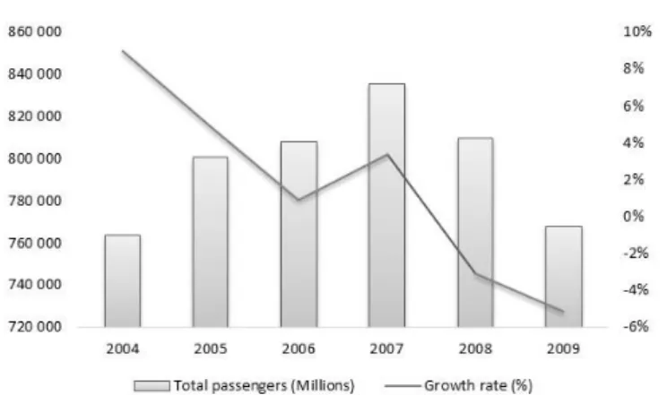
The passenger transport is the primary source of the US airline industry accounting for 52% of the total operating revenue of this industry in 2009 (Fig. 2). A significant percentage of the passenger transport’ revenues comes from the domestic market that represents the major segment accounting for 80,5% of the 768 million passengers transported in 2009. From these total, 50% were transported by the top four airlines in terms of number of domestic passengers transported (Fig. 1) while the top ten represents 83% of the total passengers. The remaining 19,5% represents the international market in which the top ten airlines were responsible by the transportation of 52% of the total international segment’ passengers, being evident the competition of foreign carriers in this market (App. 4).
Figure 1: Top airlines in terms of domestic passengers transported-2009
Source of data: Bureau of Transportation Statistics T-100 Market data. Percentages calculated by the author.
A common productivity’ measure of an airline firm is the revenue passenger miles (RPM’s) that can be compared with the available seat miles (ASM’s) in order to calculate the overall passenger load factor. In 2009, the top 10 airline with both higher RPM’s and ASMs are all major airlines (App. 5) representing 83% and 86% of the total industry’ RPM’s and ASM’s respectively.
Figure 2: Components of the industry’ operating revenue and operating expenses in 2009
Source of data: Bureau of Transportation Statistics. Percentages calculated by the author.
Besides the passenger transportation, there are other revenue sources in this industry namely the freight/cargo transportation that individually accounts for 24% of the industry’ operating revenue in 2009 (Fig. 2). In these segment there are airlines leaders such as the FedEx and the UPS that exclusively transport cargo however, the passenger airlines also compete in this segment but in a small percentage with the top five passenger airlines representing only 21% (US DOT and ATA) of the total industry revenue ton mille (App. 6)
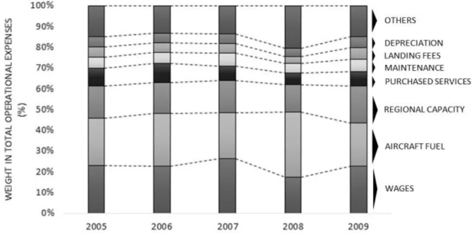
Concerning with the expenses, the flying operations expenses, which includes the fuel, represent 35% of the total operating expesnses of the industry in 2009 (Fig. 2) being the most significant component. Due the significant percentage of these expenses the industry is pretty exposure to fluctuations in the material and supplies prices (IBES 2011). Individually, the fuel expenses represents 21% of the total operating expenses of the US airlines industry demonstrating the importance of this component in this industry.
3.1.2. Competition environment
The US Airlines industry was deregulated in 1978 allowing the entrance of several low-cost carriers (LCCs). These airlines with a lower cost structure contributed for a higher competition and forced the established network legacy carriers (NLCs) to reformulate their strategies in order to maintain their market share (Belobaba et al. 2011).