UNIVERSIDADE DE LISBOA
FACULDADE DE CIÊNCIAS
DEPARTAMENTO DE FÍSICA
Modeling and design of an electromagnetic actuation system for the
manipulation of microrobots in blood vessels
Patrícia Alexandra Afonso Zoio
Dissertação
Mestrado Integrado em Engenharia Biomédica e Biofísica
Perfil em Engenharia Clínica e Instrumentação Médica
UNIVERSIDADE DE LISBOA
FACULDADE DE CIÊNCIAS
DEPARTAMENTO DE FÍSICA
Modeling and design of an electromagnetic actuation system for the
manipulation of microrobots in blood vessels
Patrícia Alexandra Afonso Zoio
Dissertação orientada por:
Professora Doutora Rita G. Nunes
Professor Doutor Hugo A. Ferreira
Mestrado Integrado em Engenharia Biomédica e Biofísica
Perfil em Engenharia Clínica e Instrumentação Médica
i
Abstract
Navigation of nano/microdevices has great potential for biomedical applications, offering a means for diagnosis and therapeutic procedures inside the human body. Due to their ability to penetrate most materials, magnetic fields are naturally suited to control magnetic nano/microdevices in inaccessible spaces. One recent approach is the use of custom-built apparatus capable of controlling magnetic devices. This is a promising area of research, but further simulation studies and experiments are needed to estimate the feasibility of these systems in clinical applications.
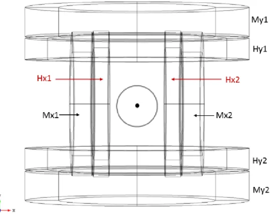
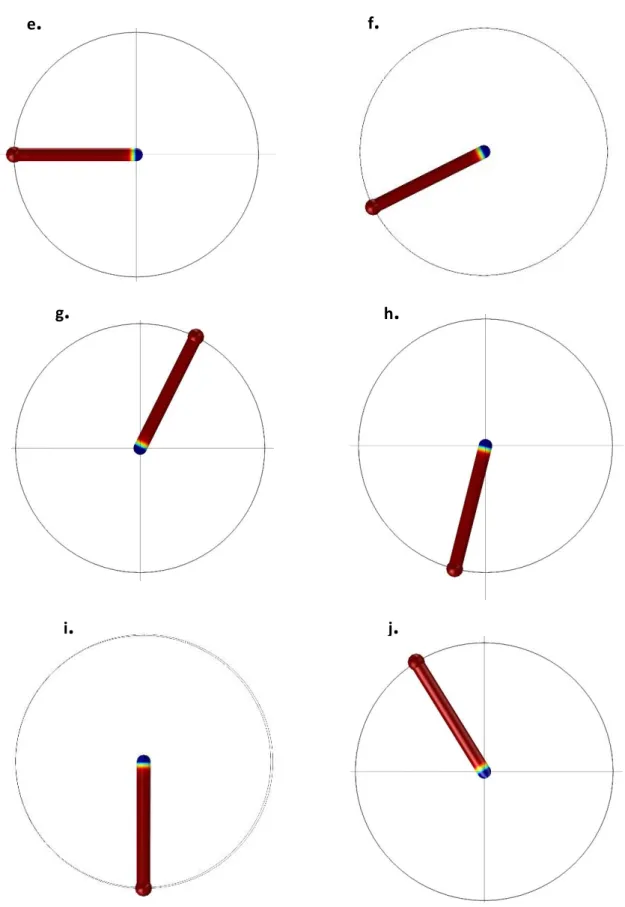
The goal of this project was the simulation and design of an electromagnetic actuation system to study the two dimensional locomotion of microdevices. The first step was to identify, through finite element analysis using software COMSOL, different coil configurations that would allow the control of magnetic devices at different scales. Based on the simulation results, a prototype of a magnetic actuation system to control devices with more than 100 𝜇m was designed and built from the ground up, taking into account cost constraints. The system comprised one pair of rotational Helmholtz coils and one pair of rotational Maxwell coils placed along the same axis. Furthermore, additional components had to be designed or selected to fulfil the requirements of the system. For the evaluation of the fabricated system, preliminary tests were carried out. The locomotion of a microdevice was tested along different directions in the x-y plane.
The simulations and experiments confirmed that it is possible to control the magnetic force and torque acting on a microdevice through the fields produced by Maxwell and Helmholtz coils, respectively. Thus, this type of magnetic actuation seems to provide a suitable means of energy transfer for future biomedical microdevices.
iii
Resumo
A navegação de nano/microdispositivos apresenta um grande potencial para aplicações biomédicas, oferecendo meios de diagnóstico e procedimentos terapêuticos no interior do corpo humano. Dada a sua capacidade de penetrar quase todos os materiais, os campos magnéticos são naturalmente adequados para controlar nano/microdispositivos magnéticos em espaços inacessíveis. Uma abordagem recente é o uso de um aparelho personalizado, capaz de controlar campos magnéticos. Esta é uma área de pesquisa prometedora, mas mais simulações e experiências são necessárias para avaliar a viabilidade destes sistemas em aplicações clínicas.
O objectivo deste projecto foi a simulação e desenho de um sistema de atuação eletromagnética para estudar a locomoção bidimensional de microdispositivos. O primeiro passo foi identificar, através da análise de elementos finitos, usando o software COMSOL, diferentes configurações de bobines que permitiriam o controlo de dispositivos magnéticos em diferentes escalas. Baseado nos resultados das simulações, um protótipo de um sistema de atuação magnética para controlar dispositivos com mais de 100 𝜇m foi desenhado e construído de raiz, tendo em conta restrições de custos. O sistema consistiu num par de bobines de Helmholtz e rotacionais e um par de bobines de Maxwell dispostas no mesmo eixo. Além disso, componentes adicionais tiveram de ser desenhados ou selecionados para preencher os requisitos do sistema. Para a avaliação do sistema fabricado, testes preliminares foram realizados. A locomoção do microrobot foi testada em diferentes direções no plano x-y.
As simulações e experiências confirmaram que é possível controlar a força magnética e o momento da força que atuam num microdispositivo através do campos produzidos pelas bobines de Maxwell e Helmholtz, respectivamente. Assim, este tipo de atuação magnética parece ser uma forma adequada de transferência de energia para futuros microdispositivos biomédicos.
v
Acknowledgements
“If I have seen further it is by standing on the shoulders of Giants.” Isaac Newton
I would like to thank my supervisors Professor Rita Nunes and Professor Hugo Ferreira, for their helpful guidance during this work and for all the valuable advices. Both of them were a source of encouragement.
I would also like to thank Professor Maria Margarida Cruz for the gaussmeter.
A very special thanks goes to my friend Mariana for all the support since the beginning and for helping me reviewing this dissertation.
Finally, I would like to express my gratitude to my parents for encouraging me every step of the way. This thesis is dedicated to them.
vii
Contents
1. Introduction ... 1 1.1 Motivation ... 1 1.2 Dissertation Objectives... 3 1.3 Thesis Outline ... 4 2. Principles of Magnetism ... 72.1 Brief history of magnetism ... 7
2.2 Maxwell’s Equations ... 8
2.3 Magnetic materials ... 9
2.3.1 Diamagnetic materials ... 12
2.3.2 Paramagnetic materials ... 13
2.3.3 Ferromagnetic materials ... 13
2.3.3.1 Soft and hard magnetic materials ... 14
2.3.3.1.1 Permanent magnets ... 15
2.4 Electromagnetic coils... 17
2.4.1 Helmholtz and Maxwell Coils ... 18
3. Microrobotics for biomedical applications ... 23
3.1 Introduction ... 24
3.2 Potential applications of medical microrobots ... 25
3.2.1 Basic functions ... 26 3.2.1.1 Targeted therapy ... 26 3.2.1.2 Material removal ... 27 3.2.1.3 Controllable structures ... 28 3.2.1.4 Telemetry... 28 3.2.2 Application Areas ... 29 3.2.2.1 Circulatory system ... 29
3.2.2.2 Central nervous system ... 30
viii
3.3 Power and Actuation methods ... 32
3.4 Wireless Magnetic actuation ... 33
3.4.1 State-of-the-art ... 33
3.4.1.1 MRI systems for propulsion ... 34
3.4.1.2 Custom built apparatus ... 36
3.4.1.3 Modeling and Computational Tools ... 38
3.4.2 Forces acting on a microdevice ... 40
3.4.2.1 Magnetic Force and Torque ... 40
3.4.2.1.1 Magnetic dipole moment ... 41
3.4.2.1.2 Magnetically linear particle ... 42
3.4.2.1.3 Nonlinear magnetic media ... 43
3.4.2.1.4 Magnetic Torque ... 44
3.4.2.2 Hydrodynamic drag force ... 44
3.4.2.3 Apparent weight ... 46
3.5 Microrobots localization ... 46
4. Modeling ... 49
4.1 Problem description ... 50
4.1.1 Magnetic actuation of a permanently magnetized microdevice ... 54
4.1.2 Magnetic actuation of small microparticles ... 58
4.2 COMSOL Modeling ... 63
4.2.1 Magnetic actuation of microdevices ... 64
4.2.1.1 Geometry ... 64
4.2.1.2 Magnetic Fields Mode ... 65
4.2.1.3 Coefficient Form PDE ... 67
4.2.1.5 Results ... 69
4.2.1.5.1 𝑥-axis Helmholtz coils ... 70
4.2.1.5.2 𝑥-axis Maxwell coils ... 73
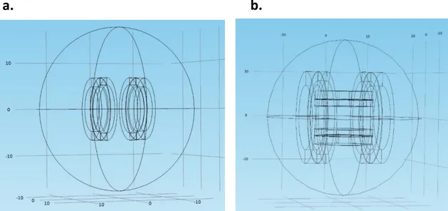
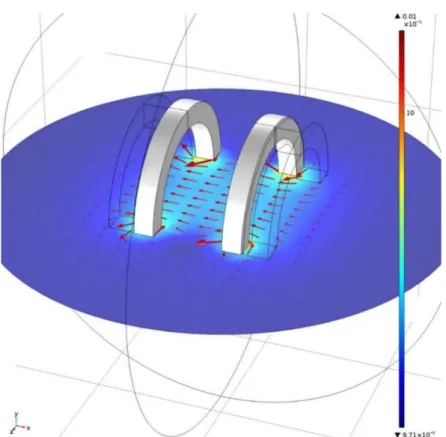
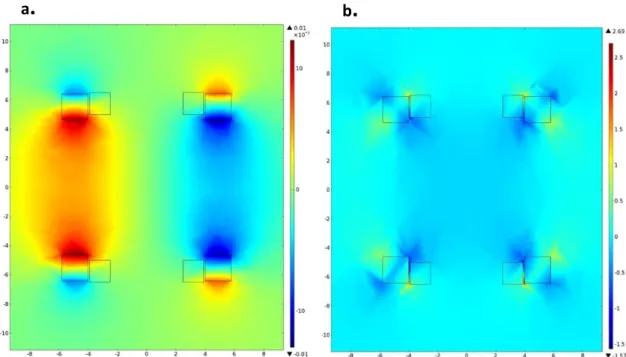
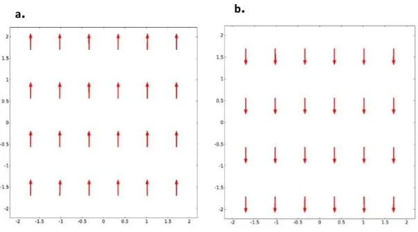
4.2.1.5.3 𝑥-axis Helmholtz and Maxwell coils ... 77
4.2.1.5.4 𝑦-axis Helmholtz and Maxwell coils ... 79
4.2.1.5.5 𝑥-axis and 𝑦-axis Helmholtz and Maxwell coils ... 81
4.2.1.6 Particle Tracing ... 83
ix
4.2.2.2 Helmholtz coils ... 91
4.2.2.3 Maxwell coils ... 93
4.2.2.4 Helmholtz and Maxwell coils ... 96
4.2.2.5 Particle Tracing ... 98 4.2.5.5.1 Results ... 101 5. Experimental Work ... 111 5.1 Problem Description ... 112 5.2 Setup Overview ... 114 5.2.1 Coils ... 115 5.2.2. Coil support ... 122
5.2.3. Wiring and microscope support ... 124
5.2.4 Electronic system ... 125
5.2.4.1 Stepper motor ... 126
5.2.4.2 Arduino and driver ... 127
5.2.4.3 Switch for current inversion ... 130
5.3 Experiments ... 131
5.3.1 Experimental setup ... 131
5.3.2 Experimental Results and Discussion ... 132
6. Conclusion and Future Work ... 139
6.1 Conclusion ... 139 6.2 Future Work ... 143 References ... 149 Appendix A ... 157 Appendix B ... 158 Appendix C ... 160 Appendix D ... 161
xi
Nomenclature
Abbreviations and Acronyms
MIT Minimally invasive therapy
MEMS Micro-electro-mechanical-systems MRI Magnetic resonance imaging EMA Electromagnetic actuation system DOF Degree of freedom
FEM Finite element modeling FEA Finite element analysis GI Gastrointestinal CT Computer tomography IR Infrared
PET Positron emission tomography ROI Region of interest
USB Universal Serial Bus GND Ground
DIY Do-it-yourself
xii 𝐻⃗⃗ Magnetic field [A/m] 𝐵⃗ Magnetic flux density [T] 𝐸⃗ Electric field [V/m] 𝜌 Free electrical charge [C/m3]
𝐽 Free current density [A/m2]
𝜇 Magnetic permeability [N/A2]
𝜇0 Magnetic permeability of free space: 4𝜋 × 10−7 N.A-2 [N/A2] 𝜇𝑟 Relative permeability of the medium
𝜒 Magnetic susceptibility
𝑚⃗⃗ Magnetic moment [A.m2]
𝑀⃗⃗ Magnetization [A/m] 𝐼 Current [A] 𝑁 Number of wire turns of a coil
𝑟,R Radius [m] 𝑑 Diameter [m] 𝐷 Distance [m] 𝐹 Force [N] 𝑉 Volume [m3] 𝐹𝑚 ⃗⃗⃗⃗ Magnetic force [N] 𝐹𝑑 ⃗⃗⃗⃗ Drag froce [N] 𝑊𝑎 ⃗⃗⃗⃗⃗ Apparent weight [N] 𝜑 Magnetic scalar potential [(V.s)/m] A Magnetic vector potential [(V.s)/m] 𝜏 𝑚 Torque [N.m] 𝜌𝑓 Density of a fluid [kg/m3]
xiii 𝐶𝑑 Drag coefficient 𝑅𝑒 Reynolds number
𝜇𝑓 Viscosity of a fluid [kg/(s.m)] λ Ratio of particle to vessel diameter
𝑚𝑝 Mass of a particle [kg]
𝐶
𝑀𝐷 Ratio of magnetic forces over drag forces 𝑤 Width [m]ℎ Height [m]
𝐷
𝑐 Diameter of the copper wire [m]𝜃 Angle [º] 𝑅 Resistance [Ω] 𝑡 Time [s]
𝑥 First world coordinate frame direction or distance [m] 𝑦 Second world coordinate frame direction [m]
𝑧 Third world coordinate frame direction [m]
1 “In the beginning there was nothing, which exploded”
-Terry Pratchett
Chapter 1
Introduction
The goal of this dissertation was to study the feasibility of a magnetic actuation system to control microrobots in blood vessels. In this chapter, the motivation behind this goal will be discussed. Also, the different objectives will be defined and the outline of the thesis will be presented.
1.1 Motivation
Cancer is a class of diseases involving unregulated cell growth. These cells can invade adjoining parts of the body and spread to other organs in a process referred to as metastasis which is one of the major causes of death. Surgery is the primary method of treatment of most isolated solid cancers. However, depending on the tumor location and the damaged caused to surrounding tissues, surgery is not always possible. Other options for cancer treatment include chemotherapy and radiotherapy. However, these treatments have many drawbacks mainly because of the difficulty in differentiating healthy and diseased tissue.
Approximately twenty years ago, there was a paradigm shift in medicine with the advent of minimally invasive therapies (MIT) [1]. Nowadays, this is an active area of research since related techniques can reach remote places without the need of open surgery, achieving better results. Some of the patient related benefits of MIT are reduced trauma, reduced infection risk, reduced postoperative pain and a faster recoveries [2].
The ability to localize, target and have a protected, prolonged and controlled interaction with the diseased tissue in the body, would allow better treatment not only for
2 cancer but many other diseases. This would allow reducing the drug or radiation dosages taken by the patient, reducing the possible side-effects.
One of the most used minimally invasive techniques is catheter embolization. It is used to treat a wide variety of conditions affecting different organs in the human body. However, it has several limitations since it is unable to reach remote areas within the cardiovascular system [3].
The use of robots in minimally invasive treatments aims to benefit medicine by further reducing treatment invasiveness in a way that until now was not possible to conceive, enabling the treatment of previously inoperable patients.
In the human body there is a large number of cavities/ canals filled with fluids (circulatory system, urinary system, central nervous system, eyes) which can be accessed through open orifices or a needle injection. It is conceivable that, in the future, robots could use this natural pathways within the body to reach its target and perform a new set of minimally invasive diagnostic, therapeutic, and surgical procedures. As technology advances, allowing further reduction in the size of these robots, their potential could increase allowing them to have a better penetration depth inside the body.
This dissertation focuses on the manipulation of microrobots. This is a very challenging area and several problems and limitations have to be studied and discussed. Specifically, power and actuation are generally some of the most challenging problems in the field of microrobotics. At this moment, due to fabrication limitations, a microrobot that it is entirely autonomous, including actuators, power source and integrated sensors is unrealistic. An alternative is to develop actuation systems capable of controlling the microrobots from a distance. One approach to the wireless control of untethered microrobots is through externally applied magnetic fields.
The design of an effective magnetic actuation system requires research in three main areas:
The development of the magnetic robot taking into account its material, geometry, and capabilities;
Real-time imaging of the magnetic devices as they move through the blood vessels;
The development of technology to propel/steer the microrobot through the circulatory system.
This dissertation focuses on the third area of research, studying the feasibility of a magnetic actuation system for microrobots control.
3
1.2 Dissertation Objectives
This dissertation had two major goals. One was to simulate, using the finite element method, different magnetic actuation systems and test the effect of their produced magnetic force on the locomotion of microdevices. The second goal was to fabricate, from the ground up, one of the simulated magnetic actuation systems. With these theoretical and experimental studies the objective was to evaluate the technical feasibility of magnetic actuation of microrobots in blood vessels, for future medical interventions.
Overall, the different sub-goals defined during this work were:
Study in detail the main forces acting on a magnetic device traveling in the blood vessels, when subjected to a magnetic force;
Perform preliminary numerical simulations using MATLAB in order to define the general requirements for the control of magnetic devices in blood vessels, at different scales;
Simulate different coil configurations that would allow the control of microrobots, through finite element analysis, using the software COMSOL and test the efficiency of these proposed systems using the Particle Tracing Module. Since the control of magnetic devices in blood vessels is very dependent on the scale of the problem, the goal was to explore two special cases, separately:
o Perform finite element simulations for designed electromagnetic actuation systems with the purpose of controlling devices that are permanently magnetized and bigger than 100 𝜇m;
o Perform finite element simulations for electromagnetic actuation systems with the purpose of controlling particles with diameters ranging from 1 𝜇m to 100 𝜇m and considering different values of saturation magnetization.
Taking into account the results from the finite element simulations, one important goal was to design and fabricate a system, from the ground up, capable of controlling permanently magnetized devices bigger than 100 𝜇m in the vessels, considering cost constraints and using a do-it-yourself approach. Next, the goal was to test the fabricated system using the available material;
Based on the results from the fabricated device and on the knowledge acquired through the simulations, the final goal was to discuss the potential and limitations of magnetic actuation and to propose a system capable of controlling particles at a smaller scale.
4
1.3 Thesis Outline
This dissertation work is presented in 6 chapters. The overall view of the dissertation is depicted in Figure 1.1.
After discussing the motivations and the objectives of this work in chapter 1, in chapter 2, the basic magnetic principles are reviewed with focus on the most relevant aspects for this work such as the study of different coil configurations.
In chapter 3, after an overview of the theoretical background of microrobotics and its potential applications in medicine, a review of the previous work related to wireless magnetic actuation is presented. Also in this chapter, the forces acting on a magnetic device in the blood vessels when subjected to magnetic field are discussed in some detail. Finally, the different possibilities for localization in vivo of microrobots are presented and discussed.
Chapter 4 starts with numerical simulations using MATLAB, to define the general requirements for the control of magnetic devices in blood vessels, at different scales. Based on these requirements, this chapter follows with the finite element analysis using the software COMSOL, showing the results of different coil configurations that would allow this control. Through the Particle Tracing Module the efficiency of these proposed systems is evaluated.
In chapter 5, the experimental work is described. First, the different components of the system, with its characteristics, functionality and constraints are discussed in some detail. Also, the magnetic field was measured to investigate the linearity and magnitude of the magnetic fields produced by the coil configuration and the results are presented and compared to the finite element model. Also in this chapter, the results from the 2-dimensional control of a millimeter-sized permanent magnet using the fabricated electromagnetic actuation system are shown and discussed.
Finally, chapter 6 summarizes the main results and findings from this dissertation and presents ideas for future projects.
5
7 “The magnetic force is animate, or imitates soul; in many respects it
surpasses the human soul while it is united to an organic body.” -William Gilbert in De Magnet, 1600
Chapter 2
Principles of Magnetism
In this work, the forces used to propel the biomedical microdevices are generated by a coil system capable of producing the desired magnetic fields. Nowadays, this and many other applications are possible due to the work of many researchers throughout history. This chapter will start with a brief history of magnetism, followed by a brief explanation of the fundamentals of magnetism, highlighting the most relevant aspects to this project.
2.1 Brief history of magnetism*
The history of the study of magnetic and electric effects is an old one, originated in Greek culture as an offspring of philosophy in 6th century B.C. Aristotle attributed the first of what could be called a scientific discussion on magnetism to the Greek philosopher Thales of Miletus, who discovered the interesting properties of Iodestone, capable of attracting iron or assuming north-south orientation. Around the same time, in ancient India, the surgeon Sushruta was the first to make use of a magnet for surgical purposes.
The first systematic experiments on magnetism did not occur until 1600 A.D. with the publication of De magnete by W. Gilbert where he concluded that the earth is magnetic. In the 18th century there were numerous and ordered observations of magnetic and electric
phenomena mainly by D. Bernoulli, H. Cavendish, Ch. A. Coulomb, B. Franklin, A. Galvani and A. Volta. Also, the refinement of mathematical analysis introduced by I. Newton and G.W. Leibniz in 1670-75, and extended by L. Euler and J. L. Lagrange in 1744-55 contributed to the progress in the study of electromagnetic phenomena.
8 In 1820, the physicist Oersted discovered the connection between electrical current and magnetic field when a current-carrying conductor near a compass caused the compass needle to deflect. The mathematician A.M. Ampère was stimulated by Oersted’s discovery and, within a few months, he extended both experimentally and theoretically the understanding of magnetic effects related to electric currents. For this work Ampère is considered by many to be the “father” of electromagnetism. In 1826, G.S. Ohm finally established the relation between electric field and current.
In 1831, M.Faraday described the law of induction and introduced the concept of magnetic lines of force. Throughout the following decades, several scientists and mathematicians contributed to the electromagnetism theory. In particular, electromagnetic phenomena were gradually formulated in more exact mathematical terms through the contribution of C.F. Gauss, W.E. Weber, W. Thomson, R. Kohlraush, and H. Helmholtz.
In 1855, the Scottish mathematician and physicist J.C Maxwell further extended the ideas about field lines and in 1873 his Treatise on Electricity and Magnetism was published. The contributions in 1885-85 by H. Hertz and O. Heaviside gave Maxwell’s equations their final form. In the next section (2.2) these equations will be briefly discussed in the context of this thesis.
In the first half of the 20th century, with the advent of quantum mechanics, magnetic
effects were explained considering the atomic structure of material. Classical electromagnetic theory was coupled with quantum mechanics into quantum electrodynamics.
2.2 Maxwell’s Equations
Maxwell’s equations represent the concluding highlight of centuries of discoveries and studies in electromagnetism and set the comprehensive foundation of classical electromagnetic theory. In differential form, the equations can be written as:
Gauss’s Law ∇ ∙ 𝐷⃗⃗ = 𝜌 2.1 Gauss’s Law for Magnetism ∇ ∙ 𝐵⃗ = 0 2.2 Faraday’s Law of Induction ∇ × 𝐸⃗ = −𝜕𝐵⃗ 𝜕𝑡 2.3 Ampère’s Law ∇ × 𝐻⃗⃗ = 𝐽 +𝜕𝐷𝜕𝑡⃗⃗ 2.4
9 In the above equations, 𝐻⃗⃗ (in A/m) and 𝐸⃗ (in V/m) are the magnetic and electric field respectively, 𝐷⃗⃗ (in C/m2) and 𝐵⃗ (in T) are the electric and magnetic flux density (or electric and
magnetic induction), 𝜌 (in C/m3) and 𝐽 (in A/m2) are, respectively, the free electric charge and
free current density. The nabla operator, ∇, in Cartesian coordinates is defined as: ∇= [𝜕𝑥𝜕 , 𝜕
𝜕𝑦, 𝜕 𝜕𝑧]
𝑇
Gauss’s Law is the first of Maxwell’s Equations which dictates how the electric field behaves around electric charges. This law states that a charge density is the source of the electric flux density. Gauss’s law for magnetism means that there are no “magnetic charges” analogous to electric charges. Instead, the magnetic fields due to materials are generated by a configuration called a dipole. The Maxwell-Faraday’s equation version of Faraday’s law describes how a time varying magnetic field induces an electric field. The Ampère’s law with Maxwell’s equation states that magnetic fields can be generated in two ways: by electric current and by changing electric fields. More specifically, a current density and a time-varying electric flux density cause a curl of the electric field.
In this dissertation, the special case of magnetostatics is considered. Under static conditions, there are no electric charges (𝜌 = 0), no electric fields (𝐸⃗ = 0) and the condition of static fields (𝑑𝑡𝑑 ( ∙ ) = 0) it is considered. Thus, it is possible to reduce Maxwell’s equations to equations 2.5 and 2.6.
∇ ∙ 𝐵⃗ = 0 2.5 ∇ × 𝐻⃗⃗ = 𝐽 2.6 Also, if there are no currents in the region of interest 𝐽 =0.
Equation 2.5 states that the number of field lines entering any given volume in space is equal to the number of field lines leaving that volume (the net flux of 𝐵⃗ through surface S is zero).
To make a general solution possible (of a system defined by 2.5 and 2.6) the constitutive relationship between 𝐵⃗ and 𝐻⃗⃗ , i.e, 𝐵⃗ (𝐻⃗⃗ ) of a material is required. This relationship defines the classification of magnetic materials as discussed in section 2.3.
2.3 Magnetic materials
The magnetic flux density, 𝐵⃗ is the response of a material when applying an external magnetic field, 𝐻⃗⃗ [5]. The relationship between these vectors depends on the material itself and it is given by the constitutive law:
10
𝐵⃗ = 𝜇(𝐻⃗⃗ )𝐻⃗⃗ 2.7 where 𝜇(𝐻⃗⃗ ) is the magnetic permeability tensor, which is generally anisotropic (directionally
dependent) and nonlinear. In this dissertation, linear and isotropic materials are considered. In this case, 𝜇(𝐻⃗⃗ ) reduces to a scalar:
𝐵⃗ = 𝜇 ∙ 𝐻⃗⃗ 2.8 𝜇 = 𝜇0𝜇𝑅 2.9 where the magnetic permeability of free space 𝜇0 is, by definition, 4𝜋 × 10−7Tm/A and 𝜇𝑟 (dimensionless) is the relative permeability of the media. The relative permeability can be used to classify materials into three categories: diamagnetic (𝜇𝑟 < 1), paramagnetic (𝜇𝑟 = 1 to 10) and ferromagnetic (𝜇𝑟 ≫ 10). This parameter can be seen as a measure of how well a material concentrates the flux lines. The higher the relative permeability, the more flux lines go through the material for the same magnetic field 𝐻⃗⃗ . The relative permeability for several materials can be seen in Table 2.1.
Table 2.1 Relative permeability of several materials [6].
In general, it is only possible to see an effect on materials with a large relative permeability (ferromagnetic materials) and this is the reason why they are usually referred to as “magnetic materials”. In vacuum or air, 𝜇𝑟 = 1. In this case, 𝐻⃗⃗ and 𝐵⃗ are simply related by the magnetic constant 𝜇0:
𝐵⃗ = 𝜇0𝐻⃗⃗ 2.10 Material 𝝁𝒓 Iron 4,000 Permalloy 70,000 Supermalloy 1,000,000 Permendur 5,000 Cobalt 600 Manganese-Zinc Ferrite 750 Nickel-Zinc Ferrite 650 Bismuth 0.9998 Mercury 0.9999 Copper 0.9999 Water 0.9999 Air 1.0000 Tungsten 1.0000 Manganese 1.0010
11 The properties of a magnetic material are dependent on the net magnetic moment 𝑚⃗⃗ (A.m2), which results from the presence of an external magnetic field. In magnetic materials,
the cause of the magnetic moment are the spin and orbital angular momentum states of the electrons. The magnetic susceptibility 𝜒 quantifies the tendency of a material to form magnetic dipoles. It is a dimensionless scalar related to the relative permeability 𝜇𝑟 by equation 2.11.
𝜒 = 𝜇𝑟− 1 2.11 The magnetic susceptibility of various materials can be seen in Table 2.2.
Table 2.2 Magnetic susceptibility of several materials [6].
Using equations 2.9 and 2.11, Equation 2.8 can be expressed as:
𝐵⃗ = 𝜇0(1 + 𝜒)𝐻⃗⃗ 2.12 It is an experimental fact that in most materials, when subjected to a magnetic field 𝐻⃗⃗ , an additional magnetic field component 𝑀⃗⃗ (A/m) is generated locally. This component is called magnetization vector and it is defined as the net magnetic moment per unit of volume. This vector is related to the magnetization current 𝐽⃗⃗⃗⃗ or movement of bound charges through 𝑚 equation 2.13.
𝐽𝑚
⃗⃗⃗⃗ = ∇ × 𝑀⃗⃗ 2.13 Using equations 2.6 and 2.11, the total current density 𝐽 can be expressed as:
𝐽 = 𝐽⃗⃗⃗⃗ + 𝐽𝑚 ⃗⃗⃗ 2.14 𝑓 where 𝐽⃗⃗⃗ is the current density in free space. Thus, equation 2.4 becomes: 𝑓
∇ × 𝐵⃗ = 𝜇0(𝐽⃗⃗⃗⃗ + 𝐽𝑚 ⃗⃗⃗ ) 2.15 𝑓
Material Magnetic Susceptibility𝝌
Bismuth −17.6 × 10⁻⁵ Silver −2.4 × 10⁻⁵ Copper −0.88 × 10⁻⁵ Water −0.90 × 10⁻⁵ Cabon Dioxide −1.2 × 10⁻⁵ Oxygen 0.19 × 10⁻⁵ Sodium 0.85 × 10⁻⁵ Aluminum 2.3 × 10⁻⁵ Tungsten 7.8 × 10⁻⁵ Gadolinium 48000 × 10−5 Iron 30 × 103 Iron-Nickel 80 − 300 × 103
12 Substituting equation 2.13 into equation 2.15:
∇ ×𝜇𝐵⃗
0− 𝑀⃗⃗ = 𝐽⃗⃗⃗ 2.16 𝑓 In the case of linear and isotropic materials, the relative permeability is dependent on the magnetic field intensity 𝐻⃗⃗ , with 𝐵⃗ and 𝐻⃗⃗ parallel to each other and in the same direction. As a result, magnetization can be defined as:
𝑀⃗⃗ = 𝜒𝐻⃗⃗ 2.17 Using the equations here described it is possible to define 𝐻⃗⃗ as:
𝐻⃗⃗ =𝜇𝐵⃗
0− 𝑀⃗⃗ 2.18 It is important to note that the linear relationship between 𝐻⃗⃗ and 𝐵⃗ is a simplification and only holds for sufficiently small magnetic fields. Nonlinear magnetic materials vary from equation 2.20. In these case, the relationship expressed in equations 2.11 and 2.19 implies that the magnetization vector 𝑀⃗⃗ also depends on 𝐻⃗⃗ . Thus:
𝐵⃗ = 𝜇𝐻⃗⃗ + 𝐵⃗⃗⃗⃗⃗⃗⃗⃗⃗ 2.19 𝑟𝑒𝑚 Where 𝐵⃗⃗⃗⃗⃗⃗⃗⃗⃗ = 𝜇𝑀⃗⃗ (in T) is the residual magnetic flux density (remanence). 𝑟𝑒𝑚
The magnetic properties of materials, expressed by the magnetization 𝑀⃗⃗ depend on two main atomic effects, which can give rise to large local magnetic fields: the orbital motion of electrons around the nucleus, which can be seen as current loops of atomic dimensions or as small magnetic dipole moments; the intrinsic spin of electrons (or nuclei) with the related magnetic dipole moment. The relative permeability or the magnetic susceptibility, which define 𝑀⃗⃗ , varies widely, as shown in the previous tables. In the next sections the different types of magnetic materials will be described.
2.3.1 Diamagnetic materials
Diamagnetic substances are materials where, in the absence of an external magnetic field, orbit and pin magnetic moments cancel resulting in no net magnetic moment in the material. The response to an applied magnetic field is the creation of circulating atomic currents that produce a very small bulk magnetization antiparallel to the magnetic field, causing the field 𝐵⃗ within the material to reduce slightly. The susceptibility, which is a measure of how effective an applied field is for inducing a magnetic dipole, for a diamagnetic material is negative, as can be seen in equation 2.20.
13 𝜒 = −𝑁𝑉𝜇0𝑒2
6𝑚 ∑ 〈𝑟𝑖 2〉 2.20 where N is the number of atoms, e is the charge of an electron, V is the volume, m is the mass of the electron, and 〈𝑟〉 is the average orbital radius. With a 𝜇𝑅 value less than one, diamagnetic materials experience a slight repulsive force from permanent magnets and are thus repelled. Examples of diamagnetic materials from tables 2.1 and 2.2 include: bismuth, mercury, copper, water, silver, and carbon dioxide.
2.3.2 Paramagnetic materials
Paramagnetic materials have a net angular momentum arising from unpaired electrons. In bulk material the random orientation of atoms may result in almost no net magnetic moment. In the presence of an external magnetic field, the atomic dipoles in a material will experience a torque which tends to align the magnetic moment to the applied field, producing a small increase in the field 𝐵⃗ inside the material. Upon removal of the applied magnetic fields, these materials return to their initial state. Paramagnetic materials have a value of 𝜇𝑅 slightly greater than one and a positive magnetic susceptibility. Air, tungsten, manganese, oxygen, sodium, and aluminum are examples of paramagnetic materials presented in tables 2.1 and 2.2.
2.3.3 Ferromagnetic materials
Ferromagnetic materials are the ones with the largest relative permeability (103− 105), exhibiting strong magnetic effects. In order to characterize the properties of a given ferromagnetic material, it is necessary to measure the magnetic induction 𝐵⃗ as a function of 𝐻⃗⃗ over a continuous range of 𝐻⃗⃗ to obtain the hysteresis curve. The term hysteresis, introduced by Ewing, means to lag behind and it is the most common way to represent the bulk magnetic properties of a ferromagnetic material. Alternatively, plots of magnetization 𝑀⃗⃗ against 𝐻⃗⃗ are used, however this contain the same information since 𝐵⃗ = 𝜇0(𝐻⃗⃗ + 𝑀⃗⃗ ). Figure 2.1 shows the dependence of magnetization on external fields for a ferromagnetic material. With these types of materials, when an external magnetic field is applied, the atomic dipoles align themselves with it. If the field 𝐻⃗⃗ is increased indefinitely the magnetization eventually reaches the saturation magnetization, 𝑀𝑠, a condition where all the magnetic dipoles within the material
14 are aligned in the direction of the magnetic field 𝐻⃗⃗ . The saturation magnetization is dependent on the magnitude of the atomic magnetic moments and the number of atoms per unit of volume. Upon removal of the field, a considerable fraction of the moments are still left aligned, resulting in a remanent magnetization, 𝑀𝑟 [7].
Figure 2.1. Hysteresis curve for a ferromagnetic material (M vs H) [8].
This is used to describe the remaining magnetization when the field has been removed after magnetizing to an arbitrary level. Therefore, when a magnetic field is applied to a material that displays ferromagnetic behavior and then removed, the magnetization does not follow the initial magnetization curve and this gives rise to the hysteresis loop of the material. To demagnetize the material it is necessary to apply a magnetic field 𝐻𝑐𝑖 (intrinsic coercivity) in the opposite direction of magnetization. Ferromagnetic materials are classified as either soft or hard depending on their coercivity which is a structure-sensitive magnetic property.
2.3.3.1 Soft and hard magnetic materials
Soft magnetic materials, for example iron, are characterized by their high permeability and low coercivity (Hc < 1 kA/m), thus these materials can be easily magnetized and
demagnetized by external fields. On the other hand, hard magnetic materials, for example permanent magnets, have lower permeability but high coercivity (Hc > 10 kA/m) and large
15 remanent magnetization. Thus, once magnetized, they retain their magnetization against external fields. The difference between these two materials is illustrated in Figure 2.2.
Figure 2.2. Hysteresis loops for soft and hard magnetic materials [9].
There are several applications for soft ferromagnetic materials as a result of their ability to enhance the flux produced by an electric current. Their uses are closely connected with electrical applications such as electrical power generation and transmission, receipt of radio signals, microwaves, inductors, relays and electromagnets. The most commonly used soft magnets are soft iron (widely used as a core material for electromagnets), alloys of iron-silicon, nickel-iron, and soft ferrites. When selecting a soft material, the most important properties are its permeability, saturation magnetization, resistance and coercivity.
Hard magnetic materials, due to its characteristics, are suitable for applications such as permanent magnets and magnetic recording media.
2.3.3.1.1 Permanent magnets
A permanent magnet is a passive device used for generating a magnetic field. It is obtained by applying to a hard ferromagnetic material a field pulse that runs from zero up to when saturation induction is obtained, and back to zero. Permanent magnets deliver magnetic flux into a region of space called the air gap, with no expenditure of energy.
In recent years, a permanent magnet material based on neodymium-iron-boron has been discovered. This has superior magnetic properties for many applications when compared
16 with its predecessor samarium-cobalt. As can be seen in table 2.3, its coercivity can be as high as 1120 kA/m compared with 696 kA/m for samarium-cobalt.
In addition to the coercivity another parameter of prime importance to permanent magnet users is the maximum energy product (BH)max. This is obtained by finding the
maximum value of the product |BH| in the second, or demagnetizing, quadrant of the hysteresis loop. It represents the magnetic energy stored in a permanent magnet material.
The great advantage of permanent magnets is that they maintain a magnetic field without any power input, as it happens with electromagnets. For practical reasons, the field must remain as much as possible unaffected by time, temperature, and imposed outer field variations. These properties can be obtained with the correct choice of ferromagnetic material, which must possess, among other properties: a) A large energy product defined in the upper left quadrant of the hysteresis curve; b) a large value of magnetization M or remnant induction Br; c) a large value of the coercive field Hc (to avoid canceling the remaining induction. Typical
parameters of some hard ferromagnetic materials suitable for the construction of permanent magnets are given in Table 2.3. The most important uses of permanent magnets are in electric motors, generators and actuators. In this dissertation, a permanent magnet made of this material was used as the microdevice to be controlled.
17 2.21 2.22 2.23
2.4 Electromagnetic coils
The Bio-Savart Law is an equation used for computing the magnetic field generated at an arbitrary point by a steady current. It states that the magnetic field 𝐵⃗ from a wire length 𝑑𝑠 , carrying a steady current 𝐼, is given by equation 2.21.
𝐵⃗ = 𝜇0 4𝜋∫
𝐼𝑑𝑠 × 𝑟̂ 𝑟3
where 𝜇0 is the permeability of free space, 𝑟̂ is the displacement unit vector in the direction pointing from the wire element towards the point at which the field is being calculated and r is the radius. This equation allows the calculation of the magnetic fields for arbitrary current distributions such as circular or rectangular loops.
The magnitude of the magnetic field 𝐵⃗ along an axis through the center of a circular loop as shown in Figure 2.3, carrying steady current 𝐼 can be expressed as:
𝐵(𝑧) = 𝜇0𝐼𝑅
2𝑁
2(𝑟2+ 𝑧2)3⁄2
Where r is the radius of the loop and N is the number of turns in the current loop.
The direction of the magnetic field at the center is perpendicular to the plane of the loop, and the direction is given by the right hand rule for a current loop: fingers curls around the loop in the direction of the current, the thumb points in the direction of the magnetic field at the center of the loop. At the center of the loop (N=1), when z=0, the magnetic field is given by equation 2.23.
𝐵 =𝜇0𝐼 2𝑟
Figure 2.3. Single circular coil with radius r, carrying an electrical current I.
I
r
18
2.24
2.25
2.4.1 Helmholtz and Maxwell Coils
Considering two identical circular loops of radius r, separated by a distance D, and carrying the same current in the same direction as can be seen in Figure 2.4. The magnetic field produced by these two loops is the sum of the fields produced by the individual loops.
Figure 2.4. Two identical circular loops with radius r, separated by a distance D, carrying the same
current in the same direction. P is an arbitrary point at a distance z from their center, and at distance z1 from coil 1 and distance z2 from coil 2.
The magnetic field along their axis of symmetry at point P at a distance z from their center can be determined for each coil and the fields can be added together for the final result. If the currents in each coil are in the same direction, then the fields will complement each other to produce a strengthened magnetic field at each point.
Equation 2.24 can be used to determine the magnetic field of a pair of Helmholtz coils. Applying this equation, the magnetic fields at point P will be given by equations 2.24 and 2.25 for coil 1 and coil 2, respectively.
𝐵1= 𝜇0𝑁𝐼 2 𝑟2 (𝑟2+ 𝑧 12) 3 2 ⁄ 𝐵2 = 𝜇0𝑁𝐼 2 𝑟2 (𝑟2+ 𝑧 22)3⁄2
r
D
P
Coil 1
Coil 2
z
z
1z
219 2.26 2.27 2.28 2.29 2.30
The total magnetic field at point P will be the sum of the fields 𝐵1 and 𝐵2 and with the necessary coordinate transformations the longitudinal component of the magnetic field created by the coil pair at a distance z from the origin is obtained.
𝐵𝑧 = 𝜇0𝑁𝐼𝑟2 2 ( 1 [𝑟2+ (𝐷 2 − 𝑧) 2 ] 3 2 ⁄ + 1 [𝑟2+ (𝐷 2 + 𝑧) 2 ] 3 2 ⁄ )
Where r is the coil radius and D is the distance between the coils. It is possible to find a maximal field at the center z=0 between the coils. For that it is useful to expand 𝐵𝑧 as a Taylor series around this point. For an arbitrary function f(z):
𝑓(𝑧0+ ℎ) ≈ 𝑓(𝑧0) + ℎ𝑓′(𝑧 0) + ℎ2 2!𝑓′′(𝑧0) + ⋯ + ℎ𝑛 𝑛!𝑓(𝑛)(𝑧0) It is possible to take the first derivative of Equation 2.26 to find:
𝑑𝐵𝑧 𝑑𝑧 = 3𝜇0𝑁𝐼𝑟2 2 ( (𝐷 2⁄ − 𝑧) [𝑟2+ (𝐷 2 − 𝑧) 2 ] 5 2 ⁄ − (𝐷 2⁄ + 𝑧) [𝑟2+ (𝐷 2 + 𝑧) 2 ] 5 2 ⁄ ) Which vanishes at z=0 for any D. Taking the second derivative:
𝑑2𝐵 𝑧 𝑑𝑧2 = 3𝜇0𝑁𝐼𝑟2 2 ( 4(𝑑 2⁄ − 𝑧)2− 𝑟2 [𝑟2+ (𝑑 2 − 𝑧) 2 ] 7 2 ⁄ + 4(𝑑 2⁄ + 𝑧)2− 𝑟2 [𝑟2+ (𝑑 2 + 𝑧) 2 ] 7 2 ⁄ )
which vanishes at z=0 for D=r. Since the third derivative, like all other odd derivatives, vanished for any d, 𝐵𝑧 is uniform around z=0 up to a term of order 𝑧4
𝐵𝑧(𝑧) = 𝐵𝑧(0) + 𝑂[(𝑧/𝑑)4]
when the distance is chosen to be the same as the radius of the loops. This special configuration is called a Helmholtz coil, invented by Hermann von Helmholtz in the middle of the 19th century. This device, consisting of two identical circular magnetic coils placed symmetrically along a common axis, and separated by a distance equal to the radius of the coil as can be seen in Figure 2.5, generate a uniform constant field of magnitude 𝐵0= 𝜇𝑟0𝐼, around
20 2.31 2.32
a.
b.
the origin. The Helmholtz coil configuration has found applications in MRI as RF coils because of its ability to generate a uniform field in the vicinity of their midpoint. Figure 2.5b shows the magnetic field (𝐵𝑧) of the Helmholtz coil pair along the axis with coils of radius 5 cm and a current of 1 A.
Figure 2.5. Helmholtz coil pair a) Schematics, b) The magnetic field of the Helmholtz coil pair along the
axis with r=5 cm and I=1A (1 Gauss=1× 10⁻⁴𝑇𝑒𝑠𝑙𝑎) [11].
If the currents in the two loops are in opposite directions, with origin at the center, it is possible to calculate from the Biot-Savart law that the axial field 𝐵𝑧 is given by equation 2.31.
𝐵𝑧 = 𝜇0𝑁𝐼𝑟2 2 ( 1 [𝑟2+ (𝐷 2 − 𝑧) 2 ] 3 2 ⁄ − 1 [𝑟2+ (𝐷 2 + 𝑧) 2 ] 3 2 ⁄ )
From which it is possible to find that 𝐵𝑧, as well as all the even derivatives, vanish at z=0. Its third derivative is found to be:
𝑑3𝐵 𝑧 𝑑𝑧3 = 15𝜇0𝐼𝑟2 2 ( 4(𝐷2 − 𝑧)3− 3 (𝐷2 − 𝑧) 𝑟2 [𝑟2+ (𝐷 2 − 𝑧) 2 ] 9 2 ⁄ − 4(𝐷2 + 𝑧)3− 3 (𝐷 2 + 𝑧) 𝑟2 [𝑟2+ (𝐷 2 + 𝑧) 2 ] 9 2 ⁄ )
z
I
D=r
r
I
21
2.33
a.
b.
which vanishes at z=0 for 𝐷 =√3𝑎. At this distance, the first derivative is nonzero, therefore, 𝐵𝑧 around z=0 is linear along z up through the fourth power of z, that is:
𝐵𝑧(𝑧) = 𝐵𝑧′(0) + 𝑂[(𝑧 𝑑⁄ )5]
when the distance is chosen to be √3 times the radius of the loops. This configuration is called the Maxwell coil configuration, named in honor of the Scottish physicist James Clerk Maxwell. It is a device for producing uniform gradient magnetic flux intensity along its axis and has found applications in MRI as a gradient coil. Figure shows the configuration for a Maxwell coil pair and the resultant magnetic field (𝐵𝑧) along the axis with coils of radius 5 cm and a current of 1 A.
Figure 2.6. Maxwell coil pair a) Schematics, b) The magnetic field of the Maxwell coil pair along the axis
with r=5 cm and I=1A (1 Gauss=1× 10⁻⁴𝑇𝑒𝑠𝑙𝑎) [11].
The analysis from this chapter is important for the project since the proposed magnetic actuation systems are based on the Helmholtz and Maxwell coil configurations due to their ability to produce static magnetic fields and constant magnetic gradients, respectively. In the next chapters it will be explained how this can be used to control microrobots.
z
I
D=√𝟑r
r
23 “Man is the center of the universe. We stand in the middle of infinity
between outer and inner space, and there’s no limit to either.” -Fantastic Voyage, 1966
Chapter 3
Microrobotics for biomedical
applications
In recent years, there have been tremendous advances in the field of microrobotics. Potential applications in this field include minimally invasive diagnosis and treatment inside the human body. In this chapter, a brief review about microrobotics for biomedical applications will be presented.
It is important to start this study with some definitions. First, regarding the term robot. Although literature defines this concept in many ways, in this work it will be defined as a moving device that can make decisions by processing incoming information [12]. Thus, in the future, an untethered robot must not only have the capability to move or travel in blood vessels, but also to obtain and process information, being able to operate within specific constraints. Also, in this work, the field of microrobotics will be considered to include the design and fabrication of robots with characteristic dimensions from 1 micrometer to 1 millimeter (1000 𝜇𝑚) [13].
This chapter will start off with a brief introduction about the field of microrobotics with focus on the potential applications of microrobots in biomedicine. Afterwards, a review of the previous work related to wireless magnetic actuation will be presented. The principles governing the actuation of these devices rely on an understating of microscale physics. In this chapter, the forces acting on a microdevice navigating in the blood vessels, when subjected to a magnetic field will be presented in detail. Finally, localization in vivo of microrobots, required for feedback control and safety, will be discussed.
24
3.1 Introduction
It can be predicted that Micro-Electro-Mechanical-Systems (MEMS) technology will have an important impact in minimally invasive surgical techniques by providing untethered biomedical microrobots capable of performing new medical procedures in the human body. This idea was first presented by the physicist Richard Feynman, in 1959, in his famous lectures [14], wherein he introduced the world to the concept of “swallowing the doctor” which involved building small, swallowable surgical robots*. In 1966, the sci-fi movie Fantastic Voyage was released. In the movie, a team of scientists and their submarine are miniaturized and injected into the blood vessels of a dying man with the intention of treating a blood clot. Since its release almost 50 years ago, countless references to this film have been made in literature.
Interest in microrobotics grew rapidly in recent decades, parallel with advances in MEMS, and the results of several research groups suggest that microrobots for biomedical applications will not remain in the realm of science fiction much longer. The first studies in untethered robots were made in the 90’s, such as a swimming mechanism composed of a small magnet attached to a spiral wire [15]. In recent years, there has been significant progress especially in miniature robots (usually with a few centimeters) for use in the gastrointestinal (GI) tract [16]. Motivated by the capsule endoscopes already in clinical use, several researchers started exploring ways of expanding the capabilities of these devices, ranging from lab-on-a-chip applications equipped with several sensors (for pressure, pH, temperature) to new possible ways of locomotion. Other groups have started exploring the possibility of using smaller devices, at the microscale, in other locations in the human body. Microrobots, because of their dimensions can navigate in very narrow spaces such as blood vessels. This gives rise to a vast array of potential applications, mainly related to in vivo biomedical applications and therapy.
As the devices are scaled down to the microscale, one important concept is related to the types of physical interactions which dominate the motion and interaction of the robot. Briefly, in the case of centi/milli-scale robots the main forces are inertial and other bulk forces, while the motion of micro-scale robots is dominated by surface area-related forces (friction, adhesion, drag and viscous forces).
*According to Feynman, it was his friend and graduate student Albert Hibbs who originally suggested to him the idea of a medical use for his theoretical micromachines.
25 At sizes below tens of micrometers, effects such as Brownian motion and chemical interactions have to be considered. This is the case of nanorobots, which will not be discussed in this thesis. Nanorobots are generally envisioned as devices to target individual cells and most proposed nanosized devices are more like pharmaceuticals and less like machines, using concepts from synthetic biology and requiring large numbers to complete a task [17].
In this work, microrobots are defined as being in the size range of single to a thousand of micrometers. Thus, it is considered that they are being dominated by micro-scale physical forces and effects (this analysis will be made in detail in chapter 3.4.2). This size range presents several challenges, not only in fabrication but also in actuation and power supply. Miniature on-board power sources are one of the main problems of miniature robots, since at present there are no feasible on-board power sources for millimeter-scale robots. Also, although miniaturized actuators have been proposed, their employment for actuation of microrobots is still a problem. In chapter 3.3 this problematic will be discussed in more detail and some solutions will be explored.
In general, there is a need to take a different perspective on microrobot design and control when comparing to traditional macroscopic robots. However, even with this difficulties, this is an exciting new field and preliminary experimental results are demonstrating their feasibility for several applications. These potential applications include mobile sensor networks, micro-factories, microfluidics, bioengineering and healthcare. In this thesis, we are interested in exploring the latter.
3.2 Potential applications of medical microrobots
*According to Nelson et al. in [17], the trend in medicine is towards smaller devices and components to reduce recovery times and risks for the patients. Remote microrobots can offer a means for advanced diagnostics and therapeutic procedures inside the human body. Some of the potential application areas for medical microrobots are shown in figure 3.1. Progress in other potential medical application areas will come with the refinement of microrobot motion strategies in 3-dimensional liquid environments and with the development of relevant integrated microtools.
26
Figure 3.1 Examples of possible biomedical microrobotics applications, including targeted therapy,
telemetry, controllable structures and material removal [17].
3.2.1 Basic functions
Some simple tasks could be achieved with the use of biomedical microrobots. In the following sections possible tasks for medical microrobots are presented.
3.2.1.1 Targeted therapy
One of the main potential applications for microrobots is targeted therapy allowing the localized delivery of chemical and biological substances or other forms of energy. Possible therapeutic uses for microrobots include:
27 - Drug delivery. With this approach a pharmaceutical compound is transported in the blood vessels to safely achieve its target and performing the desired therapeutic effect, thus reducing the side effects in the rest of the body.
- Brachytherapy (internal radiotherapy). This is a form of radiotherapy where a radioactive source is placed inside or next to the area needing treatment. The radiated energy results in the destruction of the cells surrounding the radioactive source. - Hyperthermia. This is a technique involving the selective deactivation of cancer cells by
heating the damaged areas in the temperature range of 42- 45 ºC. The adverse side effects from conventional therapies and the resulting patient discomfort have encouraged researchers to explore these site-specific therapies using magnetic nanoparticles.
- Stem cell therapies. Stem cells are undifferentiated biological cells that can differentiate into specialized cells or divide to produce more stem cells. They hold enormous potential for future therapies and there’s a possibility that microrobotic assistance will be needed.
3.2.1.2 Material removal
Another potential application of microrobots is to remove biological material by mechanical means. Possible methods of material removal using microrobots include:
- Ablation. This process consists on the removal of material from the surface of an object by erosive processes. This can be achieved using the rotary motion of microrobots, which could be useful, for example, in the treatment for atherosclerosis through the removal of fatty deposits from the internal walls of blood vessels. It could also be possible to use ultrasound ablation, in which the microrobot uses a resonating mechanical structure to emit ultrasonic pressure waves to destroy an object such as a kidney stone.
- Biopsy. This is an intervention involving sampling of cells or tissues for examination. This intervention could be performed by microrobots. Also, in the future, it could also be possible to combine the excision with remote-sensing technology. Thus, the sample could be analyzed in situ.
28
3.2.1.3 Controllable structures
It could also be possible to use microrobots as simple structures whose positions are controllable. Some examples of this type of applications include:
- Tissue scaffolds, which act as cell support frames. The microrobot itself can act as a scaffold, or the microrobots can deploy the building blocks which will act as a scaffold. - Stents. These are mesh tubes inserted into a natural passage in the body to prevent or
counteract a disease-induced, localized flow constriction. A stent can be used, for example, to keep blood flowing through a clogged vessel. The microrobot could serve as a stent and would navigate and deploy in the targeted location.
- Occlusions. This can be introduced to intentionally block a passageway. A potential future application could be to use microrobots which could function as occlusions, for example, to clog a blood vessel that nourishes a tumor.
- Electrodes for medical purposes. These electrical conductors can be introduced by microrobots, which could operate wirelessly. The microrobot could act as a permanent or temporary implant which could be useful for many purposes, for example, for brain stimulation.
3.2.1.4 Telemetry
Telemetry is the communication process in which measurements are made and other data collected at remote or inaccessible points and transmitted to receiving equipment for monitoring. Microrobots can be used to transmit information that otherwise would be difficult (or impossible) to obtain. Some of the applications of microrobots in the area of telemetry include:
- Remote sensing. Microrobots could transmit the time history of a physical signal of interest or transmit a simple binary signal upon detecting the presence of an analyte of interest.
- Marking a specific location. This could be useful specially when combined with remote sensing to localize unknown internal phenomena (for example, bleeding). To perform this task, the microrobots must be able not only to sense and transmit information but also to maintain its location at the site.
29
3.2.2 Application Areas
Some of the targeted areas of the body could include the circulatory system, central nervous system, urinary tract, and the eye.
3.2.2.1 Circulatory system
The essential components of the human circulatory system are the heart, blood, and blood vessels. The blood vessels are the conduits responsible for the transport of the blood throughout the body. The three major types of blood vessels are: the arteries, which carry the blood away from the heart, the capillaries, which enable the exchanges of substances between the blood and the tissues, and the veins, which carry blood from the capillaries back toward the heart. Figure 3.2 shows a schematic representation of various types of blood vessels, with the inner diameter, average blood-flow speed and Reynolds number. The Reynolds number is a dimensionless number that relates the effects of inertial forces to those of viscous forces on a fluid and it is used to determine the flow regime of the flow (laminar or turbulent). Generally, in the body, blood flow is laminar; however, under conditions of high flow, laminar flow can be disrupted and become turbulent. When this happens, blood does not flow linearly and smoothly in adjacent layers, but instead the flow can be described as being chaotic [18].
The circulatory system could be the most important application area for wireless microrobots since nearly every site of the body can be accessed by the blood vessels. Some possible applications are target drug delivery, lysis of blood clots (thrombolysis) and the use of microrobots acting as stents to maintain blood flow.
Figure 3.2 Schematic representation of the vessels of the cardiovascular system, with the inner diameter,
30
3.2.2.2 Central nervous system
The central nervous system consists of two major structures: the brain and the spinal cord. These structures are bathed in the cerebrospinal fluid, a colorless body fluid with properties similar to water. It acts as a cushion or buffer for the brain’s cortex, providing a mechanical and immunological protection to the brain. The cerebrospinal fluid occupies the subarachnoid space and the ventricular system around and inside the brain and spinal cord. It constitutes the content of ventricles, cisterns, and sulci of the brain, as well as the central canal of the spinal cord. These structures can be seen in figure 3.3.
Craniotomy is a surgical operation in which a bone flap is temporarily removed from the skull to access the brain. This type of procedure is highly invasive, usually performed on patients who are suffering from brain lesions. This procedure can also allow doctors to surgically implant deep brain stimulators for the treatment of epilepsy and Parkinson’s disease. Untethered microrobots have the potential to dramatically affect central nervous system interventions. For example, it could be possible to insert a microrobot in the subarachnoid space, in a similar process to the lumbar puncture and navigate the device to the brain for intervention. This procedure would be much less invasive. Recently, in [20], this concept of using percutaneous intraspinal navigation was applied to brain surgery, using catheters.
Research has been made to develop wireless manipulation of magnetic seeds in the brain for the purpose of hyperthermia [21]. Also, in [22], Kósa et al. proposed a swimming microrobot for endoscopic procedures in the subarachnoid space of the spine. In [23], the use of several MEMS devices for neurosurgery which could be incorporated into a wireless microrobot was proposed.
Figure 3.3 Schematic representation of the ventricle system, a set of cavities in the brain where the
31
3.2.2.3 Urinary system and prostate
The urinary system consists of the two kidneys, ureters, the bladder, and the urethra.
In [25], Edd et al. proposed a microrobot that could swim up the ureter and destroy kidney stones. This process could have several potential benefits and would result in less harm to the kidneys. Also, MEMS devices designed for use in urology could be incorporated in the microdevices [26].
Another potential application for biomedical microrobots is in the treatment of prostate cancer. The current treatments may involve surgery (radical prostatectomy) and radiation therapy including brachytherapy. This involves the insertion of a needle through the perineum which is a difficult process in part due to the fact that the prostate deforms and moves due to the force of the needle. As a result, the radioactive seed may be released in a location different than planned. Also, during the insertion of the needle there is a risk of damaging to the surrounding nerves. An untethered microrobot could offer a minimally invasive access to the prostate though the urethra and carry a radioactive seed to the tumor site, improving the effectiveness and reducing the chances of nerve damage.
3.2.2.4 The eye
The human eye is made of three layers. The outermost layer is composed of the cornea and sclera, the middle layer consists of the choroid, ciliary body and iris and the innermost layer is the retina. It is in the latter structure that the microrobots could be more promising since retina health is critical for vision and current retinal microsurgery is both difficult and risky.
Some of the possible applications of intraocular microrobots are therapies for retinal vein occlusions, detached retinas, and epiretinal membranes, as well as diagnosis.
In [27], Yesin et al. proposed a microrobot for intraocular procedures, controlled wireless with magnetic fields and visually tracked through the pupil. In [28], Dogangil et al. proposed a method of targeted drug delivery based on diffusion from a surface-coated microrobot. In [29], Hollingan et al. proposed magnetic particles in the form of ferrofluid to act as a tamponading agent in magnetic fluid therapies designed to alleviate retinal detachments and other types of retinopathy.
![Figure 3.4 a) Preliminary experimental setup installed inside a 1.5T Siemens Magnetom Vision MRI bore [43]; b) In vivo automatic navigation of a 1.5-mm ferromagnetic bead inside the carotid artery of a living swine](https://thumb-eu.123doks.com/thumbv2/123dok_br/15128552.1010508/53.892.130.767.114.359/preliminary-experimental-installed-siemens-magnetom-automatic-navigation-ferromagnetic.webp)
![Figure 4.8 Hysteresis cycle of the magnetization of magnetite powder at room temperature (298+-0.2K) [77].](https://thumb-eu.123doks.com/thumbv2/123dok_br/15128552.1010508/80.892.216.661.378.714/figure-hysteresis-cycle-magnetization-magnetite-powder-room-temperature.webp)