WORKING PAPER SERIES
CEEAplA WP No. 04/2005
Returns to Schooling in a Dynamic Model
Corrado Andini
Returns to Schooling in a Dynamic Model
Corrado Andini
Research Fellow
Universidade da Madeira (DGE)
Working Paper n.º 04/2005
Março de 2005
CEEAplA Working Paper n.º 04/2005
Março de 2005
RESUMO/ABSTRACT
Returns to Schooling in a Dynamic Model
The paper develops a dynamic approach to Mincer equations. It is shown that a
static model is based on the restrictive hypotheses that the total return to
schooling is constant over the working life and independent of bargaining
issues. A dynamic approach allows to show that the total return to schooling of
a new labor-market entrant positively depends on his/her bargaining power as
employee; the total return increases at a decreasing rate in the first part of the
working life and depends of bargaining issues; afterwards it becomes roughly
constant and independent of bargaining. The main implication is that a static
model may produce distorted empirical results when using data on young
workers since unable to account for the pattern of the total return to schooling in
the first part of the working life. I show the latter using data from the U.S.
National Longitudinal Survey of Youth (1980-1987) and analyzing the impact of
education on within-group wage inequality a la Martins and Pereira (2004a).
However, a static model does not produce distorted empirical results when
using data on relatively experienced workers. I show the latter using Portuguese
data from the European Community Household Panel (1994-2001).
Keywords: Returns to Education, Wage Inequality, Quantile Regressions.
JEL Classification: C29, J31, I21.
Corrado Andini
Universidade da Madeira
Departamento de Gestão e Economia Campus da Penteada 9000-390 Funchal Portugal
Returns to Schooling in a Dynamic Model
First version: December 4th 2004 This version: March 19th 2005
Corrado Andini* University of Madeira
Department of Management and Economics Campus da Penteada 9000-390
Funchal Portugal
ABSTRACT
The paper develops a dynamic approach to Mincer equations. It is shown that a static model is based on the restrictive hypotheses that the total return to schooling is constant over the working life and independent of bargaining issues. A dynamic approach allows to show that the total return to schooling of a new labor-market entrant positively depends on his/her bargaining power as employee; the total return increases at a decreasing rate in the first part of the working life and depends of bargaining issues; afterwards it becomes roughly constant and independent of bargaining. The main implication is that a static model may produce distorted empirical results when using data on young workers since unable to account for the pattern of the total return to schooling in the first part of the working life. I show the latter using data from the U.S. National Longitudinal Survey of Youth (1980-1987) and analyzing the impact of education on within-group wage inequality a la Martins and Pereira (2004a). However, a static model does not produce distorted empirical results when using data on relatively experienced workers. I show the latter using Portuguese data from the European Community Household Panel (1994-2001).
Keywords: Returns to Education, Wage Inequality, Quantile Regressions. JEL Classification: C29, J31, I21.
* Financial support by the European Commission (EDWIN Project, HPSE-CT-2002-00108), the University of Madeira and the University of Salerno is gratefully acknowledged. This paper uses data from the European Community Household Panel in the version of December 2003 (the usual disclaimer applies). I sincerely thank Pedro Telhado Pereira, Santiago Budria and the participants at the 6th Meeting of the EDWIN Project for their valuable comments (the usual disclaimer applies).
Contents
1. Introduction
2. Related literature
3. Theory behind a static Mincer equation
4. From a static to a dynamic model
5. Empirical model
6. Estimation results using data on young workers
7. Estimation results using data on experienced workers
8. Implications of model specification and data
9. Conclusions Appendix A Appendix B References Tables Figures
1. Introduction
The paper develops a dynamic approach to Mincer equations. I will argue that a static model is based on the restrictive hypotheses that the total return to schooling is constant over the working life and independent of bargaining issues. A dynamic approach allows to show that the total return to schooling of a new labor-market entrant positively depends on his/her bargaining power as employee; the total return increases at a decreasing rate in the first part of the working life and depends of bargaining issues; afterwards it becomes roughly constant and independent of bargaining. The main implication is that a static model may produce distorted empirical results when using data on young workers since unable to account for the pattern of the total return to schooling in the first part of the working life. I will show the latter using data from the U.S. National Longitudinal Survey of Youth (1980-1987) and analyzing the impact of education on within-group wage inequality a la Martins and Pereira (2004a). However, a static model does not produce distorted empirical results when using data on more experienced workers. I will show the latter using Portuguese data from the European Community Household Panel (1994-2001).
The reminder of the paper is as follows. Section 2 briefly describes some common features of the literature using human-capital regressions. Section 3 describes the theory behind a static Mincer equation. Section 4 develops a theory for a dynamic Mincer equation. Section 5 presents empirical models. Sections 6 and 7 present estimation results. Section 8 deals with implications of model specification and data. Section 9 concludes the manuscript.
2. Related literature
Building on Mincer (1974), several studies have estimated the following wage equation:
(1) lnwt =α+βs+δz+φz2+εt
where lnwrepresents the logarithm of hourly earnings, s is schooling years, z is labor market experience and ε is an error term. Most of existing studies share three common features:
• the estimated models have a static nature (i.e. they do not allow for at least one lagged
value of the dependent variable as additional regressor);
• the estimated coefficient of education is dependent on number and type of explanatory
variables added to model (1) 1 (see Martins and Pereira, 2004b);
• estimation is generally based on ordinary least squares, instrumental variables, random
effects.
In this paper, I attempt to do a step onwards with respect to the current “state of the art”. The aim of this paper is to study returns to schooling in a dynamic framework. From an empirical point of view, this mainly involves keeping the autoregressive nature of earnings into account. In doing so, I also deal with the problem of choosing “control-regressors” by replacing the whole set of explanatory variables suitable to be added to model (1) with one lagged value of earnings (this approach may be extended to more than one lag). Finally, building on Martins and Pereira (2004a), I take a quantile regression approach. From a theoretical point of view, the transition from a static to a dynamic model involves re-thinking the theory behind the standard Mincer equation (1), allowing for bargaining issues to play a more important role.
1
This is done in order to improve the “explanation” of earnings and increase the “reliability” of the estimated coefficient of schooling.
3. Theory behind a static Mincer equation
The aim of this Section is to present the theoretical foundations of the standard static Mincer equation, following Heckman and Todd (2003). In Section 4, I will discuss the assumptions needed for the transition from a static to a dynamic model.
Mincer (1974) argues that observed earnings are a function of potential earnings net of human capital investment costs, and potential earnings depend on investments in previous period. If we denote potential earnings at time t as E , we can assume that, in each period t, an t individual invests in human capital a share k of his/her potential earnings with a return of t r . t Therefore we have that:
(2) Et+1 =Et(1+rtkt)
which, after repeated substitution, becomes:
(3)
∏
− = + = 1 t 0 j 0 j j t (1 rk )E E .Taking logarithms, we get the following expression:
(4)
∑
− = + + = 1 t 0 j j j 0 t lnE ln(1 rk ) E ln .If we define schooling as the number s of years spent in full-time investment, i.e. 1
k ...
k0 = = s−1 = (we assume that schooling starts at the beginning of the life), we assume that the return to schooling is constant over time, i.e. r0 =...=rs−1=β, and we assume that the return to post-schooling investment is constant too, i.e. rs =...=rt−1 =λ, then we can write (4) in the following way:
(5)
∑
− = λ + + β + + = 1 t s j j 0 t lnE sln(1 ) ln(1 k ) E ln ,which yields to:
(6)
∑
− = λ + β + ≈ 1 t s j j 0 t lnE s k E ln .for small beta, lambda and key.
In order to build up a link between potential earnings and labor market experience z, Mincer (1974) further assumes that post-schooling investment linearly decreases over time, that is:
(7) − η = + T z 1 ks z
where z=t−s≥0, T is the length of working life (independent of s) and η is between 0 and 1. Therefore, we can re-arrange expression (6) and get:
(8) 2 0 t z T 2 z T 2 s E ln E ln ηλ − ηλ + ηλ + β + ηλ − ≈ .
However, we are interested in potential earnings net of investment costs, which are given by:
(9) t 0 z2 T 2 z T T 2 s E ln T z 1 E ln ηλ − η + ηλ + ηλ + β + η − ηλ − ≈ − η − .
Finally, assuming that observed earnings are equal to potential earnings net of investment costs, i.e.: (10) − η − = T z 1 E ln w ln t t ,
and using expression (9), we obtain an expression that is very closed to the standard Mincer equation: (11) t 0 z2 T 2 z T T 2 s E ln w ln ηλ − η + ηλ + ηλ + β + η − ηλ − ≈ or (12) lnwt ≈α+βs+δz+φz2, where α=lnE0−ηλ−η, T T 2 η + ηλ + ηλ = δ and T 2 ηλ − = φ .
Hence, after inserting an error term, we get the standard model (1).
To conclude this Section, it is worth noticing that the total return to schooling in model (12) is given by the following expression:
(13) ≈β ∂ ∂ = ∂ ∂ + s w ln s w ln t s z .
Expression (13) implicitly assumes that the total return to schooling is constant over the working life since it is always equal to β for every value of labor-market experience z from 0 to T. In addition, the total return is clearly independent of bargaining issues, which are left outside of the classic construction of the static Mincer equation.
4. From a static to a dynamic model
Several authors have argued, in several ways, that model (1) is too parsimonious and that there is a need of inserting additional regressors, in order to improve the “explanation” of
earnings and get a more “reliable” estimate of the coefficient of schooling. Therefore, model (1) has been modified in the following way:
(14) lnwt =α+βs+δz+φz2+τ1ω1+τ2ω2+...τNωN +εt
where variables ω are new explanatory variables, such as sectors of activity, firm size, firm age, bargaining regimes, seniority, and so on (see Martins and Pereira, 2004b, p. 526). However, the choice of the variables to be added to model (1) is quite controversial and, more important, the estimated coefficient of schooling seems to be dependent on researcher’s choice of ω variables. From an empirical point of view, the transition from a static to a dynamic model mainly involves recognizing that earnings have auto-regressive nature and then assuming that ω1,ω2,...,ωN (which should be used to improve the “explanation” of
t
w
ln ) can be fully replaced by lnwt−1 (our reasoning can be extended to more than one lag of earnings).
However, there is also a more elegant way to go from a static to a dynamic model. It consists of modifying Mincer’s assumption (10) such that current observed earnings are a weighted average of past observed earnings and current potential earnings net of investment costs. Then equation (10) becomes: (15) t t (1 )lnwt 1 T z 1 E ln w ln + −ρ − − η − ρ = .
Expression (15) can be derived as the exact solution of a Nash-bargaining maximization problem, once we assume that:
• the employee maximizes earnings growth, namely Ut =lnwt −lnwt−1, • potential earnings net of investment costs are equal to actual productivity,
• the employer maximizes profits, namely t t lnwt
T z 1 E ln V − − η − = .
Under these assumptions, we have the following standard Nash-bargaining maximization problem2: (16) t t t w ln V ln ) 1 ( U ln max ρ + −ρ
where ρ is the bargaining power of the employee between 0 and 1, 1−ρ is the bargaining power of the employer, while (15) is the solution of (16) as shown in Appendix A.
If we use expression (9) to replace net potential earnings in equation (15), we get:
(17) lnwt ≈(1−ρ)lnwt−1+ρ
(
α+βs+δz+φz2)
or
2
(18) lnwt ≈(1−ρ)lnwt−1+ρα+ρβs+ρδz+ρφz2
It is worth noticing that, if we set ρ=1 (i.e. the employee has full bargaining power), then expression (18) becomes (12).
A particular feature of model (18) is the possibility to draw the pattern of the total return to schooling over the working life, if numerical expressions for β and ρ are available. As assumed in Section 3, an individual stops schooling at time s− (i.e. after s years, beginning 1 from year 0), starts working at a time s and receives an hourly wage equal tow . Particularly, s a new labor-market entrant maximizes Us =lnws −lnw, where lnw is the logarithm of the minimum hourly wage3, set by law. Therefore, at time s, expression (15) becomes:
(19) lnws =ρ
(
lnEs −η)
+(1−ρ)lnw.This involves that model (18), at time s, can be written as follows:
(20) lnws ≈ρα+(1−ρ)lnw+ρβs+ρδ(0)+ρφ(0)2 and the return to schooling at time s is given by:
(21) ≈ρβ ∂ ∂ s w ln s .
under the reasonable assumption that 0 s w ln = ∂ ∂ .
Expression (21) may be seen as the entry return to schooling, i.e. the return to schooling that an individual receives when enters the labor-market. It is worth noticing that it depends positively on the bargaining power of the new entrant as employee. In addition, (21) is lower than (13) except in the particular case of ρ=1.
A time s+1, we have the following:
(22) lnws+1≈ρα+(1−ρ)lnws +ρβs+ρδ(1)+ρφ(1)2 and the total return to schooling is given by:
(23) +ρβ≈ −ρ ρβ+ρβ ∂ ∂ ⋅ ρ − ≈ ∂ ∂ + ) 1 ( s w ln ) 1 ( s w ln s 1 s .
At time s+2, we have the following:
(24) lnws+2 ≈ρα+(1−ρ)lnws+1+ρβs+ρδ(2)+ρφ(2)2 and the total return is given by:
3
(25)
[
−ρ ρβ+ρβ]
+ρβ≈ −ρ ρβ+ −ρ ρβ+ρβ ρ − ≈ ≈ ρβ + ∂ ∂ ⋅ ρ − ≈ ∂ ∂ + + ) 1 ( ) 1 ( ) 1 ( ) 1 ( s w ln ) 1 ( s w ln 2 1 s 2 s .Therefore, at time s+z, the total return to schooling is given by:
(26) +ρβ≈ −ρ ρβ+ −ρ ρβ+ +ρβ ∂ ∂ ⋅ ρ − ≈ ∂ ∂ + + − − ... ) 1 ( ) 1 ( s w ln ) 1 ( s w ln s z s z1 z z 1 .
We may call expression (26) as the dynamic total return to schooling after z years of labor-market experience. It is worth noticing that (26) gives the static total return (13) as a particular case when the employee has full bargaining power (ρ=1). In general, the left-hand side of expression (26) is z-dependent and (26) allows to draw the total return to schooling over the entire working life, from 0 to T years of experience.
For a value of ρ≠1, say ρ~, we have the following:
(27) ≈β ρ − − β ρ ≈ ∂ ∂ + ∞ → 1 (1 ~) ~ s w ln lim s z z .
Therefore, under some general conditions, a dynamic model is able to provide a measure of the total return to schooling which is comparable with expression (13). We may call expression (27) as dynamic convergent total return to schooling. Expression (27) is pretty important because it shows that, if ρ≠1, a rough equivalence between a static and a dynamic model only holds at very high values of z. In other words, if the employee does not have full bargaining power, a static model does not produce an appropriate measure of the total return to schooling at relatively low values of labor-market experience. Finally, the lower is the ρ~ is, the slower is the process of adjustment of the total return from its entry value to its convergent value, the higher the z needed for a rough equivalence.
In general, as a simulation in Figure 1 shows, the dynamic total return to schooling may have a pattern, in the first part of the working life, which cannot be approximated by means of a constant line and a static model, if used to measure the total return of young workers, may produce a distorted output. A technical explanation is provided in Appendix B.
5. Empirical model
Based on expression (12) and on expression (18), I estimate the following two empirical models:
(28) lnwit =αθ+βθsi+δθzi+φθzi2+εit
(29) lnwit =γθ +υθlnwit−1+πθsi +χθzi +ςθzi2+εit
where θ goes from 0 to 1 and represents the wage distribution quantile. As model (29) is linear in parameters, individual unobserved heterogeneity is disregarded, and we focus “on the case of iid innovations in which conditioning variables play the classical role of shifting
the location of the conditional density of y [the autoregressive variable], but they have no t effect on the conditional scale or shape” (Koenker and Xiao, 2004, p. 3), then we can apply the standard quantile estimation techniques due to Koenker and Bassett (1978).
Particularly, model (29) can be written as a simple linear model:
(30) lnwi =xi'ψθ +εi with Quantθ
(
lnwixi)
=xi'ψθand the lagged logarithm of earnings can be treated as any standard explanatory variable x. An example of this approach is provided by Koenker (2000) who applies the standard quantile techniques to a first-order autoregressive model for maximum daily temperatures in Melbourne (Australia). Another example is provided by Girma and Gorg (2002) who present a more sophisticated quantile regression model where the autoregressive variable is total factor productivity.
Thus, the vector of parameters ψ is estimated as: θ (31) ψθ = ψ
∑
ϑθ − ψθ θ i i i x ' ) w (ln min arg ˆand ϑθ(ε)is the usual check function defined as ϑθ(ε)=θε when ε is non-negative or ε
− θ = ε
ϑθ( ) ( 1) when ε is negative. The same procedure applies to model (28).
Our discussion will continue as follows. First, I will present estimation results based on model (29), focusing on π and υ for each decile. As expression (21) suggests, I will refer to the estimated π as entry return to schooling. Instead, the estimated υ measures the bargaining power of the employer in model (18)4. If the “true” theoretical model behind regression (29) looks like model (18), then we should find that the estimated π is negatively correlated with the estimated υ over the wage distribution. Afterwards, following Martins and Pereira (2004a), I will present decile estimates of β in model (28), which are expected to be higher than estimates of π . I will refer to the estimated β as static total return to schooling. In addition, I will present estimates of the dynamic total return to schooling as provided by expression (26), for each decile and over the working life. Finally, I will compare the estimated total static return to schooling β with the estimated dynamic convergent total return to schooling as provided by expression (27).
6. Estimation results using data on young workers
In my first application of model (28) and of model (29), I use data from the U.S. National Longitudinal Survey of Youth for the period of 1980-1987, as provided by Verbeek (2000). The same data-set is also used by Vella and Verbeek (1998) to study union premia. The sample contains 4360 annual observations on 545 young male workers. I therefore assume, a
la Martins and Pereira, absence of participation issues typically arisen for women. Summary sample statistics for the selected variables are reported in Table 1.
Disregarding - for a moment - the quantile approach, model (29) can be estimated by OLS. Indeed, since we assume absence of individual unobserved heterogeneity, the OLS estimator is consistent. We therefore present, as a benchmark, several OLS estimates. In particular, Table 2 shows that the entry return is almost a half of the static total return, which is
4
consistent with (13) and (21) on a theoretical basis5 and with the stylized fact (see Martins and Pereira, 2004b) that addition of control-regressors (in our case, one lag of the logarithm of earnings) to model (28) deeply reduces the estimated coefficient of education, specially when the control-regressor is an education-dependent covariate (like in our case). In addition, Figure 3 plots the dynamic total return over the working life, starting from the entry year. It is increasing, at decreasing rate, during the first part of the working life; afterwards, it becomes roughly constant. This is a pretty interesting and new empirical result, which can only be obtained using a dynamic model. Finally, the dynamic convergent total return is almost equal to the static total return, because the average experience in the sample (6.51) is enough to support a static model (the dynamic total return in Figure 3 is roughly equal to its convergent value from roughly z = 6 onwards).
Another interesting point, that may be briefly discussed before presenting the main empirical results of this paper, is about the hypothesis of absence of individual unobserved heterogeneity (a la Martins and Pereira). If we continue disregarding the quantile approach and introduce individual fixed effects in model (29), than the OLS estimator becomes inconsistent (based upward; see Nickell, 1981). Estimating this new model would require implementation of the well-known GMM techniques by Arellano and Bond (1991) or by Blundell and Bond (1998), that give consistent estimates. However, as the variable s (years of schooling) does not generally vary - for the same individual - over time6, then the quoted GMM techniques, based on first differences, will inevitably drop the variable of education out of the model, together with individual unobserved heterogeneity (which is the only required outcome)7. Finally, it is worth noticing that, in every model not explicitly taking individual fixed effects into account, the presence of a lagged value of the dependent variable as additional explanatory variable is likely to reduce the role of individual unobserved heterogeneity (adding several lags of the dependent variable as regressors may make unobserved heterogeneity becoming insignificant8).
Let us now come back to a quantile approach. Figure 2 plots, over the wage distribution, the estimated bargaining power of the employer and the entry return to schooling (see also Table 2). The estimated bargaining power of the employer increases till to the forth decile and decreases till to the ninth decile. This pattern can be explained by looking at heterogeneity of jobs in terms of wage, job stability, number of potential job-applicants, and so on. For instance, we may think that the forth decile involves the best combination of these elements (which gives the highest bargaining power to the employer) while the ninth involves the worst combination. A more interesting finding is that the estimated bargaining power of the employer (employee) is negatively (positively) correlated9 with the estimated entry return to schooling, which is consistent with model (18) on a theoretical basis. Our testing rejects the hypothesis of a constant entry return to schooling over the wage distribution and shows that this return has a flat U-shape. The returns from the third to the seventh decile are roughly equal but lower than those estimated for the second and the eighth decile, which are roughly equal and, in turn, lower than the roughly equal returns for the first and the ninth decile.
5
It is worth stressing that the estimate of the entry return provided by model (29) can be roughly obtained as product between the bargaining power of the employee implicitly estimated by model (29) and the coefficient of schooling estimated by model (28). This is consistent with expression (21).
6
This is the case in our sample. In general, interviewed individuals are those who work and stopped schooling; hence they are likely to declare the same years of schooling from the first to the last annual interview.
7
However, the quoted GMM techniques may be suitable for studying returns to education for working-students.
8
See Arellano (2003) for a testing procedure.
9
Figure 2 also plots the static total return and involves two comments. First, the estimated static total return is higher than the entry return (see also Table 2). Once again, as for the OLS estimation, this is consistent with our theoretical predictions and with the stylized fact that addition of education-dependent covariates (in our case, one lag of the logarithm of earnings) to model (28) deeply reduces the estimated coefficient of education. Second, the estimated static total return is found to increase over the wage distribution10, which is consistent with the main empirical result by Martins and Pereira (2004a).
Finally, Figure 2 plots the dynamic convergent total return over the wage distribution and involves two further comments. First, it is clearly decreasing from the first to the seventh decile and a bit increasing from the seventh to the ninth. Second, it is higher than the static total return for lower-than-median wage groups while lower than the static one for higher-than-median wage groups. This raises the question of why the OLS estimation gives as outcome that the static total return is roughly equal to the dynamic convergent total return, while the QR estimation does not. In our view, this is because the average experience in the sample is high enough to support a static model, but the average experience in several deciles is not high enough to do the same, and the static model produces distorted empirical results because a constant return is unable to account for some very big “jumps” (see the first deciles in Figure 3) at low values of experience.
7. Estimation results using data on experienced workers
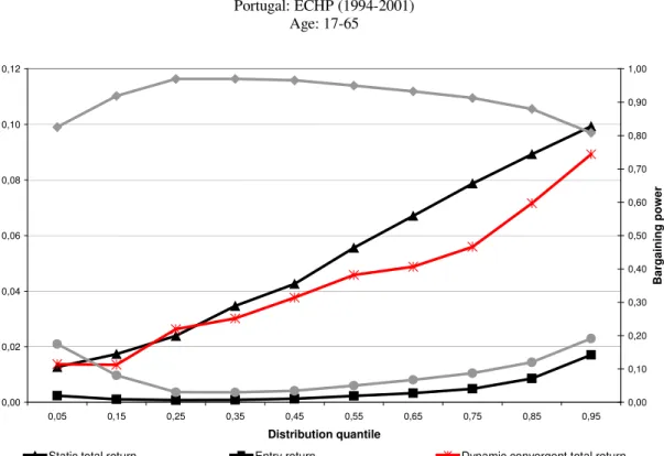
The European Community Household Panel (ECHP) is a very large data-set containing micro-data for 15 countries of the European Union from 1994 to 2001. We focus on Portugal. To build up our sample, we start extracting Portuguese data (country 12) on personal identification numbers (pid), age (pd003), gender (pd004), monthly gross earnings (pi211mg), years of education (pt023), weekly hours of work (pe005). We repeat this operation for each of the eight waves of the ECHP and construct a preliminary data-set with 91437 observations. Afterwards we drop individuals older than 65 or younger than 15 years, drop females, drop individuals still at school and those not providing information about education, create a variable for labor-market experience (lme = pd003 – pt023 – 6), drop individuals with negative experience, drop individuals with zero or missing earnings. Finally, we obtain an unbalanced panel with 15049 observations, which is described in Table 1.
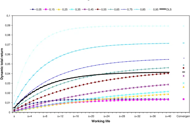
Figure 4 plots the estimation results using techniques described in Section 5 and confirms that the entry return to schooling is lower than the static total return and positively associated with the implicitly estimated bargaining power of the employee. In addition, we find that the dynamic convergent return to schooling is consistent with the static total return over the wage distribution and when using ordinary least squares. Detailed estimation results are provided in Table 2. Figure 5 plots the dynamic total return for several quantiles.
As a further confirmation, Figure 6 plots estimation results when using a sub-sample of Portuguese workers between the ages of 17 and 30, summarized in Table 1. Detailed estimation results are provided in Table 2. As expect, a static model seems to give distorted empirical results, even when using ordinary least squares due to a very low average experience (4.81). Instead, when using a sub-sample of Portuguese workers between the ages of 31 and 65 described in Table 1, a static model seems to perform properly. Table 2 provides detailed estimates.
10
This is not straightforward. However our testing shows that the ninth decile exhibits a significantly higher return than the first decile.
8. Implications of model specification and data
Summarizing my findings, I obtain results that are consistent with those of Martins and Pereira (2004a) both when estimating a static model a la Martins and Pereira and when estimating a dynamic model with data on relatively experienced workers. However, when estimating a dynamic model with data on young workers, I get a different picture of the impact of education on within-group wage inequality. Why? We will come back to this question after briefly reviewing the main arguments used by Martins and Pereira (2004a) in order to explain their result that the return to schooling increases over the wage distribution. The main explanations are three: over-education, interaction between schooling and ability, and quality of schooling. Over-education basically refers to people with high schooling levels (in terms of years) who take low-paid jobs. If there are many over-educated in the first decile of the wage distribution, then the return to an additional year of schooling will be very low. If the number of over-educated decreases over the wage distribution (as the wage increases), then the return to education is expected to increase over the wage distribution. The same reasoning holds for ability or school quality. If people ability or school quality increase over the wage distribution, then the return to an additional year of schooling should follow the same pattern.
These explanations are appealing and provide a theoretical background to understand the empirical result that the total return to schooling increases over the wage distribution in 15 of 16 countries examined by Martins and Pereira (2004a), with Greece as unique exception due to the use of after-tax earnings (i.e. the general result is distorted because of the influence of taxation). In my view, however, the general empirical result that the total return to schooling increases over the wage distribution is not robust to the use of data on young workers. A static model, indeed, is based on two restrictive hypotheses: the total return to schooling is constant of the working-life and independent of bargaining issues11. However, a dynamic model shows that the total return to schooling is not constant over the working life. It becomes constant once a certain work-experience is matured, but it is increasing in the first part of the working life and, during this period, its evolution depends on bargaining issues. If a static model is used to estimate the total return to schooling for young workers, it may give a wrong picture because the photography is related to a changing situation and the static model is not able to account for it. Finally, it is worth stressing that the latter critique does not affect the validity of empirical results by Martins and Pereira (2004a), as these authors use of data on relatively experienced workers (around 20 years).
To conclude, we suggest carefulness when using a static model to estimate the total return to schooling with data on young workers.
9. Conclusions
The paper has developed a dynamic approach to Mincer equations. I have argued that a static model is based on the restrictive hypotheses that the total return to schooling is constant over the working life and independent of bargaining issues. A dynamic approach allows to show that the total return to schooling of a new labor-market entrant positively depends on his/her bargaining power as employee; the total return increases at a decreasing rate in the first part of the working life and depends of bargaining issues; afterwards it becomes roughly constant and independent of bargaining. The main implication is that a static model may produce distorted empirical results when using data on young workers since not able to account for the pattern
11
The estimation of a static quantile Mincer equation allowing for individual fixed effects would be a further interesting exercise. A recent attempt of introducing individual fixed effects into a quantile regression framework is due to Koenker (2004).
of the total return to schooling in the first part of the working life. I have shown the latter using data from the U.S. National Longitudinal Survey of Youth (1980-1987) and analyzing the impact of education on within-group wage inequality a la Martins and Pereira (2004a). However, a static model does not produce distorted empirical results when using data on relatively experienced workers. I have shown the latter using Portuguese data from the European Community Household Panel (1994-2001).
Appendix A
This appendix solves problem (16), which is given by the following expression:
(A1) t t t w ln V ln ) 1 ( U ln max ρ + −ρ where Ut =lnwt −lnwt−1 and t t lnwt T z 1 E ln V − − η − = .
It is worth noticing that our objective function comes from a standard Cobb-Douglas. We
make a logarithmic transformation in order to make our life easier.
Once definitions of U and t V are replaced in expression (A1), we get: t
(A2)
(
)
t t t 1 t t w ln w ln T z 1 E ln ln ) 1 ( w ln w ln ln max − − η − ⋅ ρ − + − ⋅ ρ − .The maximization problem in (A2) implies the following first-order condition:
(A3) ( 1) 0 w ln T z 1 E ln 1 ) 1 ( ) 1 ( w ln w ln 1 t t 1 t t = − ⋅ − − η − ⋅ ρ − + + ⋅ − ⋅ ρ − .
After adjusting (A3), we come up with the following expression:
(A4) t t 1 t t lnw T z 1 E ln 1 w ln w ln − − η − ρ − = − ρ −
which, in turn, gives:
(A5) t lnwt (1 )
(
lnwt lnwt 1)
T z 1 E ln = −ρ ⋅ − − − − η − ⋅ ρ .Therefore, we obtain the following equation:
(A6) t lnwt (1 )lnwt (1 )lnwt 1 T z 1 E ln −ρ = −ρ − −ρ − − η − ρ
(A7) t lnwt lnwt lnwt (1 )lnwt 1 T z 1 E ln −ρ = −ρ − −ρ − − η − ρ . or (A8) t lnwt (1 )lnwt 1 T z 1 E ln = − −ρ − − η − ρ .
Finally, we get expression (15) in the main text, i.e.:
(A9) t (1 )lnwt 1 lnwt T z 1 E ln + −ρ = − η − ρ − .
Appendix B
As shown in the main text, expression (26) gives the dynamic total return to schooling, that is:
(B1) +ρβ≈ −ρ ρβ+ −ρ ρβ+ + −ρ ρβ+ρβ ∂ ∂ ⋅ ρ − ≈ ∂ ∂ + + − − ) 1 ( ... ) 1 ( ) 1 ( s w ln ) 1 ( s w ln s z s z1 z z 1 or (B2)
[
1 (1 ) ... (1 ) (1 )]
(z) s w ln s z z 1 z Λ ρβ ≈ ρ − + ρ − + + ρ − + ρβ ≈ ∂ ∂ + − .Therefore, a general static model is given by the following expression:
(B3) lnws+z ≈α+ρβΛ(z)s+δz+φz2.
Expression (B3) is equivalent to model (12) only if
(B4)
ρ ≈ Λ(z) 1 .
However, expression (B4) only holds as z tends to infinity since:
(B5) ρ ≈ Λ ∞ → 1 ) z ( lim z .
In general, we may define a function ι(z) providing the difference between Λ(z) and its convergent value ρ 1 , that is: (B6) (z) 1−Λ(z) ρ = ι .
Then, using (B6), we may write expression (B3) as follows:
(B7) lnws+z ≈α+βs+δz+φz2−ρβι(z)s .
Finally, expression (B7) allows to show that both OLS and QR estimation of the empirical static model (28) are more likely to produce biased empirical results at low z levels. Indeed, we may notice that the assumptions:
(B8) Expect
(
εs+zz,s)
=0 (OLS) and(B9) Quant
(
εs+zz,s)
=0 (QR)are more likely to be violated at low z levels since ι(z)is more likely to be significantly different from zero.
References
Arellano M. (2003) “Panel Data Econometrics”, Oxford, Oxford University Press.
Arellano M., Bond S.R. (1991) “Some Tests of Specification for Panel Data: Monte Carlo Evidence and An Application to Employment Equations”, Review of Economic Studies, 58, pp. 277-297.
Blundell R.W., Bond S.R. (1998) “Initial Conditions and Moment Restrictions in Dynamic Panel Data Models”,
Journal of Econometrics, 87, pp. 115-143.
Girma S., Görg H. (2002) “Foreign Direct Investment, Spillovers and Absorptive Capacity: Evidence from Quantile Regressions”, GEP Working Papers, University of Nottingham, n. 2002/14.
Heckman J., Todd P. (2003) “Fifty Years of Mincer Earnings Regressions”, NBER Working Papers, National Bureau of Economic Research, n. 9732.
Koenker R. (2000) “Quantile Regression”, in: Fienberg and Kadane (eds.), International Encyclopedia of the
Social Sciences, Amsterdam, North-Holland.
Koenker R. (2004) “Quantile Regression for Longitudinal Data”, Journal of Multivariate Analysis, 91, pp. 74-89.
Koenker R., Bassett G. (1978) “Regression Quantiles”, Econometrica, 46(1), pp. 33-50. Koenker R., Xiao Z. (2004) “Quantile Autoregression”, unpublished manuscript.
Martins P.S., Pereira P.T. (2004a) “Does Education Reduce Wage Inequality? Quantile Regression Evidence from 16 Countries”, Labour Economics, 11, pp. 355-371.
Martins P.S., Pereira P.T. (2004b) “Returns to Education and Wage Equations”, Applied Economics, 36, pp. 525-531.
Mincer J. (1974) Schooling, Experience and Earnings, Cambridge, National Bureau of Economic Research. Nickell S. (1981) “Biases in Dynamic Models with Fixed Effects”, Econometrica, 49(6), pp. 1417-1426. Vella F., Verbeek M. (1998) “Whose Wages Do Unions Raise? A Dynamic Model of Unionism and Wage Rate Determination for Young Men”, Journal of Applied Econometrics, 13, pp. 163-183.
Table 1
United States: NLSY (1980-1987)
Variable Obs Mean Std. Dev. Min Max Logarithm of hourly wage 4360 1.64 0.53 –3.57 4.05 Years of schooling 4360 11.76 1.74 3.00 16.00 Experience 4360 6.51 2.82 0.00 18.00
Age 4360 24.28 2.77 17.00 30.00
Portugal: ECHP (1994-2001)
Variable Obs Mean Std. Dev. Min Max Logarithm of hourly wage 13717 6.44 0.54 2.49 9.28 Years of schooling 16263 15.59 5.69 9.00 57.00 Experience 16263 16.87 11.86 0.00 49.00 Age 16263 38.47 11.52 17.00 65.00
Full sample: 17-65
Portugal: ECHP (1994-2001)
Variable Obs Mean Std. Dev. Min Max Logarithm of hourly wage 4356 6.22 0.39 2.49 8.78 Years of schooling 4934 14.47 2.66 9.00 24.00 Experience 4934 4.81 3.49 0.00 14.00
Age 4934 25.29 3.10 17.00 30.00
Restricted sample: 17-30
Portugal: ECHP (1994-2001)
Variable Obs Mean Std. Dev. Min Max Logarithm of hourly wage 9361 6.54 0.57 3.01 9.28 Years of schooling 11329 16.08 6.52 9.00 57.00 Experience 11329 22.13 10.28 0.00 49.00 Age 11329 44.21 8.81 31.00 65.00
Table 2
United States: NLSY (1980-1987) Distribution decile Bargaining power of the employer Entry return Static total return Dynamic convergent total return 0.1 0.7591 0.0404 0.0884 0.1677 0.2 0.8036 0.0292 0.0954 0.1486 0.3 0.8201 0.0220 0.0954 0.1222 0.4 0.8231 0.0214 0.1004 0.1209 0.5 0.7911 0.0216 0.1036 0.1033 0.6 0.7660 0.0219 0.1066 0.0935 0.7 0.7017 0.0224 0.1070 0.0750 0.8 0.6298 0.0326 0.1058 0.0880 0.9 0.4789 0.0511 0.1072 0.0980 OLS 0.5786 0.0447 0.1021 0.1061 Age 17-30 17-30 17-30 17-30
All estimated coefficients are significant at 1% level
Portugal: ECHP (1994-2001) Distribution quantile Bargaining power of the employer
Entry return Static total return Dynamic convergent total return 0.05 0.8253 0.7166 0.8523 0.0024 0.0181 0.0030 0.0127 0.0442 0.0084 0.0137 0.0638 0.0203 0.15 0.9188 0.8571 0.9271 0.0011 0.0080 0.0011 0.0174 0.0575 0.0119 0.0135 0.0559 0.0151 0.25 0.9696 0.9177 0.9803 0.0008 0.0037 0.0006 0.0239 0.0617 0.0174 0.0263 0.0449 0.0305 0.35 0.9702 0.9165 0.9791 0.0009 0.0041 0.0007 0.0347 0.0664 0.0266 0.0302 0.0491 0.0335 0.45 0.9655 0.8914 0.9732 0.0013 0.0040 0.0011 0.0426 0.0654 0.0366 0.0376 0.0368 0.0410 0.55 0.9498 0.8712 0.9600 0.0023 0.0060 0.0022 0.0556 0.0719 0.0500 0.0458 0.0465 0.0550 0.65 0.9324 0.8500 0.9443 0.0033 0.0077 0.0027 0.0671 0.0805 0.0617 0.0488 0.0513 0.0485 0.75 0.9125 0.8094 0.9265 0.0049 0.0098 0.0040 0.0787 0.0882 0.0746 0.0560 0.0514 0.0544 0.85 0.8800 0.7640 0.8993 0.0086 0.0147 0.0067 0.0893 0.0963 0.0848 0.0716 0.0622 0.0665 0.95 0.8085 0.6449 0.8349 0.0171 0.0288 0.0134 0.0993 0.1008 0.0956 0.0892 0.0811 0.0812 OLS 0.8873 0.7567 0.9097 0.0047 0.0133 0.0036 0.0450 0.0763 0.0383 0.0419 0.0546 0.0399 Age 17-65 17-30 31-65 17-65 17-30 31-65 17-65 17-30 31-65 17-65 17-30 31-65
Significant at 5% level Significant at 10% level Non-significant Remaining estimated coefficients are significant at 1% level
Figure 1
Simulation based on β=0.10 and ρ=0.20
0,00 0,02 0,04 0,06 0,08 0,10 0,12 s s+4 s+8 s+12 s+16 s+20 s+24 s+28 s+32 s+36 s+40 Convergent Working life D y n a m ic t o ta l re tu rn
Figure 2
United States: NLSY (1980-1987) Age: 17-30 0,00 0,02 0,04 0,06 0,08 0,10 0,12 0,14 0,16 0,18 0,1 0,2 0,3 0,4 0,5 0,6 0,7 0,8 0,9 Distribution decile R e tu rn 0,00 0,10 0,20 0,30 0,40 0,50 0,60 0,70 0,80 0,90 B a rg a in in g p o w e r
Entry return Static total return Dynamic convergent total return
Figure 3
United States: NLSY (1980-1987) Age: 17-30 0,00 0,02 0,04 0,06 0,08 0,10 0,12 0,14 0,16 0,18 s s+4 s+8 s+12 s+16 s+20 s+24 s+28 s+32 s+36 s+40 Convergent Working life D y n a m ic t o ta l re tu rn 0,1 0,2 0,3 0,4 0,5 0,6 0,7 0,8 0,9 OLS
Figure 4 Portugal: ECHP (1994-2001) Age: 17-65 0,00 0,02 0,04 0,06 0,08 0,10 0,12 0,05 0,15 0,25 0,35 0,45 0,55 0,65 0,75 0,85 0,95 Distribution quantile R e tu rn 0,00 0,10 0,20 0,30 0,40 0,50 0,60 0,70 0,80 0,90 1,00 B a rg a in in g p o w e r
Static total return Entry return Dynamic convergent total return
Figure 5 Portugal: ECHP (1994-2001) Age: 17-65 0 0,01 0,02 0,03 0,04 0,05 0,06 0,07 0,08 0,09 0,1 s s+4 s+8 s+12 s+16 s+20 s+24 s+28 s+32 s+36 s+40 Convergent Working life D y n a m ic t o ta l re tu rn 0,05 0,15 0,25 0,35 0,45 0,55 0,65 0,75 0,85 0,95 OLS
Figure 6 Portugal: ECHP (1994-2001) Age: 17-30 0,00 0,02 0,04 0,06 0,08 0,10 0,12 0,05 0,15 0,25 0,35 0,45 0,55 0,65 0,75 0,85 0,95 Distribution quantile R e tu rn 0,00 0,10 0,20 0,30 0,40 0,50 0,60 0,70 0,80 0,90 1,00 B a rg a in in g p o w e r
Entry return Static total return Dynamic convergent total return
Bargaining power of the employer Bargaining power of the employee
Portugal: ECHP (1994-2001) Age: 31-65 0,00 0,02 0,04 0,06 0,08 0,10 0,12 0,05 0,15 0,25 0,35 0,45 0,55 0,65 0,75 0,85 0,95 Distribution quantile R e tu rn 0,00 0,10 0,20 0,30 0,40 0,50 0,60 0,70 0,80 0,90 1,00 B a rg a in in g p o w e r
Static total return Entry return Dynamic convergent total return