Impact evaluation of skin color, gender, and hair on the performance of eigenface, ICA, and, CNN methods

i

Impact evaluation of skin color, gender, and, hair

on the performance of EigenFace, ICA, and CNN

methods

Muhammad Ehsan Mirzaei

Project Work report presented as partial requirement for

obtaining the Masters degree in Information Management

ii

NOVA Information Management School

Instituto Superior de Estatística e Gestão de Informação

Universidade Nova de Lisboa

IMPACT EVALUATION OF SKIN COLOR, GENDER, AND HAIR ON THE

PERFORMANCE OF EIGENFACE, ICA, AND, CNN METHODS

by

Muhammad Ehsan Mirzaei

Project Work as partial requirement for obtaining the Masters degree in Information Management with a specialization in Knowledge Management and Business Intelligence

Advisor / Co Advisor: Professor Doutor Roberto André Pereira Henriques Co Advisor: Professor Doutor Flávio L. Pinheiro

iii

February 2020

DEDICATION

iv

ACKNOWLEDGEMENTS

I wish to express my deepest gratitude to my thesis committee, professor Roberto Henriques for his patient guidance, support, encouragement, and interest in my work at every stage of this thesis and professor Flávio L. Pinheiro for his effective and straightforward advice, sharing knowledge and sharpening my ideas. This thesis demonstrates your approach for my academic mentorship.

I would like to pay my special regards to Dr Mahmud Manafi for time that devoted to review my thesis and adding value to my work by putting his comment. His suggestion adds more clarity to my writing and moreover introduced desk research techniques.

I am indebted to Carina Albuquerque for her valuable advice and guidance for my work overall and specifically in the area of deep learning. Hers suggestion about neural network architecture was very straightforward and useful, demonstrating her knowledge and expertise in this fields.

v

ABSTRACT

Although face recognition has made remarkable progress in the past decades, it is still a challenging area. In addition to traditional flaws (such as illumination, pose, occlusion in part of face image), the low performance of the system with dark skin images and female faces raises questions that challenge transparency and accountability of the system. Recent work has suggested that available datasets are causing this issue, but little work has been done with other face recognition methods. Also, little work has been done on facial features such as hair as a key face feature in the face recognition system.

To address the gaps this thesis examines the performance of three face recognition methods (eigenface, Independent Component Analysis (ICA) and Convolution Neuron Network (CNN)) with respect to skin color changes in two different face mode “only face” and “face with hair”.

The following work is reported in this study, 1st rebuild approximate PPB dataset based on work done by “Joy Adowaa Buolamwini” in her thesis entitled “Gender shades”. 2nd new classifier tools developed, and the approximate PPB dataset classified based on new methods in 12 classes. 3rd the three methods assessed with approximate PPB dataset in two face mode.

The evaluation of the three methods revealed an interesting result. In this work, the eigenface method performs better than ICA and CNN. Moreover, the result shows a strong positive correlation between the numbers of train sets and results that it can prove the previous finding about lack of image with dark skin. More interestingly, despite the claims, the models showed a proactive behavior in female’s face identification. Despite the female group shape 21% of the population in the top two skin type groups, the result shows 44% of the top 3 recall for female groups. Also, it confirms that adding hair to images in average boosts the results by up to 9%. The work concludes with a discussion of the results and recommends the impact of classes on each other for future study.

KEYWORDS

ICA; Eigenfaces; PCA; CNN; ResNet152; Dark Skin; Face Recognition

vi

INDEX

1.

Introduction ... 1

1.1.

Background ... 1

1.2.

Problem statement ... 2

1.3.

Research Question ... 2

1.4.

Object of the study ... 2

1.5.

Scope of study ... 3

1.6.

Significant of study ... 3

1.7.

Summary ... 3

2.

Literature review ... 4

2.1.

Face Recognition and AI ... 4

2.2.

Generic of face recognition ... 4

2.3.

Face Recognition Approach ... 5

2.4.

Face Recognition Methods ... 5

2.4.1.

Eigenface ... 5

2.4.2.

Linear discriminate analysis (LDA) ... 7

2.4.3.

Independent Component Analysis (ICA) ... 7

2.4.4.

Elastic Bunching Graph Model (EBGM) ... 8

2.4.5.

Hidden Markove Model (HMM) ... 8

2.4.6.

Deep Learning Neuron Network (DNN) ... 9

2.5.

Benchmark Datasets ... 11

2.6.

Face Recognition bias with dark skins ... 13

2.7.

Application Area ... 13

2.8.

Summary ... 14

3.

Methodology ... 15

3.1.

Data Collection ... 15

3.2.

Software and Libraries ... 18

3.3.

Pre-Processing ... 18

3.4.

Modeling ... 19

3.4.1.

Eigenface ... 20

3.4.2.

Independet Componant Analysis (ICA) ... 22

3.4.3.

Convolutional neural network (CNN) – ResNet152... 24

vii

4.

Results and discussion ... 29

4.1.

Eigenface Result ... 29

4.2.

ICA Result ... 31

4.3.

CNN-ResNet152 Result ... 33

4.4.

Discussion ... 34

5.

Conclusions ... 37

6.

Limitations and recommendations for future works ... 38

7.

Bibliography ... 39

viii

LIST OF FIGURES

Figure 1 Face Recognition and AI

https://www.neotalogic.com/2016/02/28/artificial-intelligence-in-law-the-state-of-play-2016-part-1/ ... 4

Figure 2 Generic Face Recognition System - Zhao et al. 2003 ... 4

Figure 3 PCA tries to reduce dimensionality by finding representative component

http://sebastianraschka.com/Articles/2014_python_lda.html ... 6

Figure 4 LDA developed with aims to increase granularity within class and between classes

http://sebastianraschka.com/Articles/2014_python_lda.html ... 7

Figure 5 ICA aims to find independent component, rather than uncorrelated Introduction.... 8

Figure 6 Artificial Neural Network (ANN) vs Convolutional Neural Network (CNN) Gogul &

Kumar, 2017 ... 10

Figure 7 Evolutionary history of deep CNNs (Khan et al. 2019) ... 11

Figure 8 Steps for this experiment ... 15

Figure 9 Fitzpatrick is a method to describe and classify skin by reaction to exposure sunlight.

https://www.arpansa.gov.au/sites/default/files/legacy/pubs/RadiationProtection/Fitzp

atrickSkinType.pdf ... 16

Figure 10 Von Luschan's Chromatic Scale is a skin color classification, that use RGB system

for classification. VLC Scale (Srimaharaj, Hemrungrote, and Chaisricharoen 2016) ... 16

Figure 11 Gender population based on skin type (project work) ... 17

Figure 12 Convert RGB color to grayscale image (PPB dataset) ... 19

Figure 13 Convert Matrix to Vector ... 20

Figure 14 Covariance matrix C... 21

Figure 15 Eigen faces (project work) ... 21

Figure 16 Eigen face method process (Dinalankara 2017) ... 22

Figure 17 Independent Component (project work) ... 23

Figure 18 An overview of a convolutional neural network (CNN) architecture and the training

process. (Yamashita, Nishio, Do, & Togashi, 2018) ... 24

Figure 19 Convolution layer https://github.com/DarknetForever/cnn-primer/tree/master/1

... 24

Figure 20 Padding https://becominghuman.ai/how-should-i-start-with-cnn-c62a3a89493b

... 25

Figure 21 Max pooling http://cs231n.github.io/convolutional-networks/#pool ... 25

Figure 22 ResNet Bock prevent from bad transformation by keeping input

https://towardsdatascience.com/introduction-to-resnets-c0a830a288a4 ... 26

ix

Figure 24 Confusion matrix is one of the easiest and intuitive metrics... 27

Figure 25 Principal components variance (project work) ... 29

Figure 26 Principal components variance (project work) ... 30

x

LIST OF TABLES

Table 1 Available 2D face dataset (Aly & Hassaballah, 2015) ... 12

Table 2 Typical application area (Zhao, Chellappa, Phillips, & Rosenfeld, 2003) ... 14

Table 3 Face image distribution based on gender and country ... 17

Table 4 Skin type distribution ... 17

Table 5 Eigenface classification report with "only face" dataset (project work) ... 30

Table 6 Eigenface classification report with "face with hair" dataset (project work) ... 31

Table 7 ICA classification report with "only face" dataset (project work) ... 32

Table 8 ICA classification report with "face with hair" dataset (project work) ... 32

Table 9 CNN-ResNet152 classification report with "only face " dataset (project work) ... 33

Table 10 CNN-ResNet152 classification report with "face with hair" dataset (project work) 34

Table 11 Overall accuracy result of methods ... 35

Table 12 Achieved highest top 3 recall score based on skin type... 36

xi

LIST OF ABBREVIATIONS AND ACRONYMS

UN United Nations

ICA Independent Component Analysis LDA Linear Discriminate analysis EBGM Elastic Bunching Graph Model

HMM Hidden Markove Model

DNN Deep Neuron Network

CNN Convolutional Neural Networks ResNet Residual neural networks PPB Pilot Parliaments Benchmark VLS Von Luschan’s Chromatic Scale AI Artificial Intelligence

ML Machine Learning

NN Neural Networks

PCA Principal Component Analysis

RGB Red, Green, Blue

BSS Blind Source Separation

1

1. INTRODUCTION

1.1. B

ACKGROUND

Face recognition refers to the technology that is capable of identifying or verifying the identity of the subject in images or video. Put simply, it is a response to the question, “Whose face it is?”. Face recognition is classified under biometric applications (Tolba, El-Baz, & El-Harby, 2006). The application maps individual facial features mathematically and compares with stored records of known images. Even though the first attempts in automating face recognition date back to the 1960s, many face recognition analysis and techniques have improved in recent decades. Rapid development in recent years is due to a combination of factors: active development of algorithms, availability of large databases of facial images, and methods for evaluating the performance of face recognition algorithms (Tolba et al., 2006). As the accuracy of face recognition systems has improved it is nowadays often preferred over other traditional biometric systems that are more robust and reliable, such as iris and fingerprint.

Due to its passive nature, face recognition systems can be more appealing than other systems (Daniel, Al, & Hartnett, 2018). For example, fingerprint recognition requires the user to place his/her finger in a sensor, while iris recognition requires users to be in a precise position in front of a scanner. Face recognition only requires the subject to be in a position allowing the camera to capture a shot of the face. This advantage makes face recognition system the most user-friendly biometric modality. On the other hand, with the rise in the use of biometric systems, issues of privacy have arisen. The ability to balance between privacy and security can be a crucial aspect of face recognition.

Face recognition provides a wide variety of applications, ranging from making mug shot albums to video surveillance for law enforcement, static matching on credit cards, ATM cards and access control through face IDs for commercial applications. Camera surveillance and social networks can be highlighted as the main uncontrolled facial image applications (Aly & Hassaballah, 2015).

Despite remarkable progress in face recognition, it is still one of the most challenging areas. On 9 February 2018, New York Times published a report by Steve Lohr about face recognition bias on white skin (Lohr, 2018). This report drew attention to the fact that although current facial recognition systems accuracy can reach up to 99%, when tested with darker skin, there is a higher margin of error reaching up to nearly 35 percent for images of dark-skinned women. The Guardian published a report entitled “‘It's techno-racism’: Detroit is quietly using facial recognition to make arrests” (Perkins, 2019) raised the same issue based on Detroit police investigations. The report points out that facial recognition software misidentifies people of color and women at much higher rates in Detroit, where 83% population is black.

Another paper (Buolamwini & Gebru, 2018), demonstrates existing face dataset does not reflect the diversity in the population in order to train automatic facial analysis system. The authors found that significant gender and skin color bias persists in influential datasets. Her work revealed that the government benchmark contained only 24.6% female faces, a proportion that dropped even lower when its broken down by gender and skin type (4.4%). The skin type for this benchmark was heavily weighted towards light skin (79.6%) with males constituting 59.4% of the group.

In a broader context, if we consider the African continent as the area of the world where the majority of people have dark skin, based on United Nations (UN) world population s reports, more than 1.308

2 billion people live in this continent, representing 16.96% of world population. If we add the population of the African diaspora to this number it increases to 19.33% of world population (UN, 2019).

A recent study (Muthukumar et al., 2018) examines the impact of skin color on face recognition performance and claims that skin color is not the driver. The conclusion is reached via stability experiments that vary an image’s skin type via color theoretical methods, namely luminance mode-shift and optimal transport. They introduced hair length as the second suspect for the failure.

Although many face recognition methods have been proposed (Eigenface, ICA, LDA, EBGM, HMM, DNN), almost all the tests have been done with pre-trained commercial classifiers. Buolamwini and Gebru (Buolamwini & Gebru, 2018) used Microsoft, IBM, and Face++ APIs. Muthukumar et al (Muthukumar et al., 2018) based their report on the results of IBM Watson’s “Gender classifier” service, IBM Watson’s “deep-face-features” API and VGGFace2 that is based on CNN – ResNet50. Although CNN is considered state of the art in computer vision , there is still no consensus on which method is best. Normally the performance of different methods is depends on a set of conditions (pose, illumination, occlusion). Hence this work selects three popular methods (eigenface, Independent Component Analysis (ICA), Convolutional Neural Network (CNN)) and compares their performance.

1.2. P

ROBLEM STATEMENT

In the face of the weak performance of face recognition systems in dark skin face images and images of female faces, most research has concluded that imbalanced face data sets that do not reflect existing population diversity as the cause of the issue. Few works have looked at hair as an influencing feature in face recognition systems. In light of this finding, this thesis focuses on the performance of different methods in connection with gender and skin type and hair impact on the face recognition system.

1.3. R

ESEARCH

Q

UESTION

- How does the eigenface method perform with regard to skin type, gender, and hair?

- How does the Independent Component Analysis (ICA) method perform with regard to skin type, gender, and hair?

- How does Convolutional Neural Network (CNN) – ResNet152 method perform with regard to skin type, gender, and hair?

- Which of the three methods (eigenface, ICA, CNN) works best in relation to the three factors (skin type, hair, gender) considered?

1.4. O

BJECT OF THE STUDY

- To measure the performance of the eigenface method with regard to skin type, gender and hair.

- To measure the performance of ICA method with regard to skin type, gender and hair. - To measure the performance of CNN – ResNet152 method with regard to skin type, gender

3

1.5. S

COPE OF STUDY

The focus of this paper is to examine the performance of different face recognition approaches with dark skin. Different approaches are reviewed and three methods examined. Approximate Pilot Parliaments Benchmark (PPB) face dataset was used for this experiment that consists of images from parliament members of six countries and restored with Von Luschan’s Chromatic Scale(VLS) and Fitzpatrick scale.

The findings of this study can help us to gain insights into the causes of the poor performance of systems and recommend methods for further study or applicationin systems.

1.6. S

IGNIFICANCE OF THE STUDY

We are living in a world in which ethnic diversity is a principal characteristic. For many reasons, such as lifestyle or geographical location, different ethnic groups have specific characteristics that are distributed irregularly around the world by geographical region. This human trait causes considerable sensitivity and tension. Given the expected role of face recognition technology in the future of human life, failure in the technology can have a huge impact on transparency and accountability, and lead to a lack of confidence in systems.

This work helps to provide insight into the performance of face recognition technology, and in particular issues raised recently in relation to bias with female and dark skin.

1.7. S

UMMARY

This chapter has introduced face recognition technology and its applications. It has reviewed the evolution of this technology from its beginnings. It has discussed barriers to face recognition, and specifically bias in processing faces with dark skin, and explain the impact of this failure on the future of the technology.

In the next chapter, the literature review, we will discuss work already undertaken in this field, different methods proposed and papers that raise the issue. In chapter 3, we will discuss more mathematical aspects of selected methods (eigenface, ICA, CNN), available datasets and characteristics of each dataset. We will look Specifically at Pilot Parliaments Benchmark (PPB) dataset, and a process to rebuild it.

Chapter 4 is dedicated to discussing findings and data analysis, including further discussion about the performance of each method. Finally chapter 5, provides conclusions based on the findings and tries to answer the research questions.

4 Figure 2 Generic Face Recognition System - Zhao et al.

2003

2. LITERATURE REVIEW

2.1.

F

ACE

R

ECOGNITION AND

A

RTIFICAL

I

NTELLIGENCE

(AI)

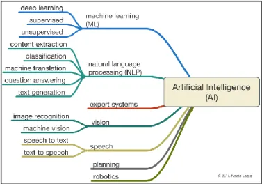
Based on NeotaLogic, AI has generated a big body of academic and commercial work. Back in 1950, John McCarthy described AI as any task performed by a machine that simulates a human carrying out the same activity. By nature, face recognition is a human behaviour that scientists could simulate by machine. In general face recognition is a subfield of computer vision but it classified under a branch of AI/Machine Learning (ML). The objective of this technology is to identify or verify persons from a digital image.

2.2. G

ENERIC OF FACE RECOGNITION

The face recognition process composed of three main modules. Although different researchers use different terminology, if we take a closer look, we find that all of them refer to the same points. Regardless of judgment about which one is better or makes more sense, I have tried to use the terms that are most intuitive for each component.

Papers (Beham & Roomi, 2013)(Zhao, Chellappa, Phillips, & Rosenfeld, 2003)(Meethongjan & Mohamad, 2007)(Hassaballah & Aly, 2015); mentioned 3 steps for a generic face recognition system.

Figure 1 Face Recognition and AI

https://www.neotalogic.com/2016/02/28/artificial-intelligence-in-law-the-state-of-play-2016-part-1/

5 ▪ Face Detection\Localization; is the process of extracting a certain image region as a face. This step has many applications such as face tracking, pose estimation and face isolation. It is the first step to extracting a certain region of the whole picture as a face.

▪ Face Normalization\Feature Extraction; is a crucial part of the system. In this step extracted features must be normalized and be independent of position, scale and rotation of face. ▪ Face Recognition\Matching is the step that represents the vector of each face that will be

matched with a known face database to identify the input face. Figure 2 shows the overall process with the application of each step.

2.3. F

ACE

R

ECOGNITION

A

PPROACH

As mentioned, face recognition is an important inner human ability, that is practised as a regular task. To build a similar computer system that performs to high satisfaction, still needs more research (Zhao et al., 2003)(Beham & Roomi, 2013).

Although Charles Darwin includes some work on “The Expression of the Emotions in Man and Animals” in 1872, the earliest work on face recognition is done in the fifties in the field of psychology (Burner and Tagiuri 1954). In the sixties Woodrow Bledsoe wrote the first engineering literature, but as his work was funded by an intelligence agency, little of his work published (Norman, 2019). The first work concerning automatic face recognition was done in 1970 by Kelly (Mahmood, Muhammad, Bibi, & Ali, 2017).

Since face recognition has been the subject of research for many years, using different methods based on different approaches, it is proposed that there is a need for a proper categorization to get an overall understanding of the concept. Various categorizations are provided for a better understanding of methods. In Paper (Zhao et al., 2003); whole face recognition methods are classified into three main groups: holistic matching method, feature-based method, and hybrid methods. Paper (Beham & Roomi, 2013) also classified into three main groups but instead of hybrid methods, introduced soft computing as the third approach. Paper (Tolba et al., 2006), used two main groups as global approaches and component-based approach.

Paper (Aly & Hassaballah, 2015), used ‘traditional’ to categorise the methods of past decades that usually are based on statistic models and ‘new’ methods that are generally based on deep learning and NN techniques.

It seems that there is no consensus for a unique classification but with a glimpse into the evolution of methods, it can be understood that all categories refer to three generic groups. 1st: methods based on features of faces, 2nd: methods based on the whole image and last or 3rd: is the method based on deep learning and soft computing. Alongside these groups, there is also a combination of these approaches known as hybrid approach.

2.4. F

ACE

R

ECOGNITION

M

ETHODS

2.4.1. Eigenface

The eigenfaces method that is known as eigenvector or Principal Component Analysis (PCA) is a method based on Karhunen-Loeve expansion in pattern recognition that was invented by Sirovich

6 and Kirby. In the paper (Sirovich & Kirby, 1987), they applied PCA to characterize the geometry of faces. Their work demonstrates that any face can be reconstructed by a representative of a coordinate system called “Eigen picture”.

Turk and Pentland (1991) proposed the Eigenface method for face detection and face recognition. The idea was motivated by the technique developed by Sirovich and Kirby (M. Turk and A. Pentland, 1991). Put simply, their method extracts relevant information in a face image, encodes it as efficiently as possible and compares it with the database of a model encoded similarly.

Mathematically, this method tries to find the principal component (PCA) of distributed faces and reduce the data space for the recognition phase (Choudhary & Goel, 2013). The input faces will convert into feature vectors and then information is obtained from the covariance matrix. These eigenvectors are used to find the variation between multiple faces. Paper (Tolba et al., 2006)(Sharif, Mohsin, & Javed, 2012) reports that, “The M Eigenfaces represent M dimensional face space showed 96%, 85% and 64% right categorization under varying lighting condition respectively, orientation and size by exploiting 2500 images of 16 each”.

In Paper (Vanlalhruaia, Yumnum Kirani Singh, & R. Chawngsangpuii, 2015), report an empirical test that uses an image database of 16 individuals and a pool total of 2500 images. The result demonstrates 96%, 85% and 64% right categorization under light variation, orientation variation, and size variation condition.

Although many experiments report good results on liner projection such as PCA but in wild situations the performance of the system is far from the ideal. Paper (Drahansky et al., 2016) states that failure is due to large illumination conditions, and facial expressions. The paper argues that the main reason is that face pattern lines on a complex nonlinear and non-convex in the high dimension. In order to deal with such cases, Kernel PCA is proposed.

Figure 3 PCA tries to reduce dimensionality by finding representative component

http://sebastianraschka.com/Article s/2014_python_lda.html

7

2.4.2. Linear discriminate analysis (LDA)

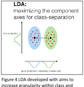
Although PCA has proved good performance, there remain critics. Paper (Belhumeur, Hespanha, & Kriegman, 1997) argued that under uncontrolled conditions, illumination and facial expression can increase the variation leading to poor discrimination. Hence, they proposed to use Linear Discrimination Analysis (LDA). LDA is based on fisher linear discrimination analysis; it is fundamentally the same as PCA, but the goal is to perform dimensional reduction while retaining class discrimination (Vanlalhruaia et al., 2015).

LDA was developed with the primary aim of increasing granularity within a class and between classes with hope to improve the recognition rate. However paper (Toygar & Introduction, 2003) reports that in the same conditions PCA recognition is higher than the LDA method.

As the LDA approach aims at maximising discrimination within classes, being resistant to illumination change can be an advantage of this method, but finding an optimum way to simultaneously separate multiple face classes is almost impossible. Also, singularity is a disadvantage for LDA. It fails when all scatter metric is singular (Kumar & Kaur, 2012).

2.4.3. Independent Component Analysis (ICA)

ICA is a generalized form of PCA, but the aim is to find independent component, rather than uncorrelated, image decomposition and representation. Theoretically, PCA is trying to find a better set of basis images that this new basis of the images are uncorrelated. But for a task like face recognition, much information is in high order relation amount the image pixels, hence ICA proposed (Bartlett, Movellan, & Sejnowski, 2002). ICA is trying to extract independent components of images by maximizing independence.

Figure 4 LDA developed with aims to increase granularity within class and between classes

http://sebastianraschka.com/Articles/20 14_python_lda.html

8 As ICA is capturing the wide spectrum of images by second-order statistics, it is expected to outperform PCA. Although this paper proves that with an experiment on FERET face date set, ICA outperforms PCA. However paper (Baek, Draper, Beveridge, & She, 2002) refutes the claim with a new test on the same data set and justifies that FERET data set was not fully available when the difference appear in result of the test. Moghaddam in (Moghaddam, 2002) claim that there is no statistical difference in the performance of the two methods.

2.4.4. Elastic Bunching Graph Model (EBGM)

Elastic Bunching Graph Model is a feature-based approach. In the context of EBGM, the image represents a graph consisting of nodes and edges. Basically, nodes represent feature points and the edge represent interconnections between nodes to form a graph like data structure (Beham & Roomi, 2013). Edges are labeled as distance, and node labels with wavelets that are locally bound into a jet(Wiskott, Fellous, Krüger, & Von der Malsburg, 1999). In this method, facial features are called fiducial points and images are represented by spectral information of regions around these fiducial points. The information is gained by convolving these portions of the image with a set of Gabor wavelet in a variety of sizes that are call Gabor JETs. By combining these represent graphs into a stack-like structure, we will have a face bunch graph. Face bunch graphs act as representatives of the face in general.

2.4.5. Hidden Markove Model (HMM)

Hidden Markov Models (HMM) is a statistical model used to characterize the statistical properties of a signal (Corcoran & Lancu, 2016). This technique was subsequently applied in practical pattern recognition applications (Stephen & Ballot, 2005). Although the HMM model was proposed in 1960 and provided a significant contribution to speech recognition (Lal et al., 2018), the first effort at face recognition was made by Samaria and Young (1994). It was extended by Nefian and Hayes (1999) and Eickeler et al (1999)(Stephen & Ballot, 2005). Samaria argues that recognition happened by discrimination of face elements (nose, mouth, eyes, etc.). Based on this logic they converted 2D image to 1D image by observing the sliding window. Each observation is a column-vector containing

Figure 5 ICA aims to find independent component, rather than uncorrelated Introduction

Presentation Introduction to ICA – University Alberta

9 the intensity level of the pixels inside the window. The sequence is formed by scanning the image in the same order (Samaria, 1995). Overall, the model has two processes. First of all is Markov Chain with a finite number of states. The second process sets the probability density function associated with it (Sharif, Naz, Yasmin, Shahid, & Rehman, 2017).

2.4.6. Deep Learning Neuron Network (DNN)

Nowadays Deep Neural Networks (DNNs) have emerged as a state-of-the-art technique in the field of machine learning. It is one of the main components of contemporary research in the field of AI (Sengupta et al., 2019). DNNs have been top performers on a wide variety of tasks including image classification, speech recognition, and face recognition (Balaban, 2015)(Beham & Roomi, 2013)(Alom et al., 2019). Many architectures proposed that based on the application, has their advantage and disadvantage. Paper (Sengupta et al., 2019) presents a collection of notable work carried out by researchers in the field of deep learning. Despite the variety of DNNs types, they try to approximate a function between input and output by changing the configuration of the net and minimizing the loss function. In general, DNNs composed of three main principal components (Balaban, 2015). The three main components that form the structure of DNNs are:

▪ The creation of some layered architectures parameterized on “Ɵ”. (Autoencoders, DNNs, CNNs, etc.)

▪ The definition of a loss functional “L”

▪ The minimization of the loss functional with respect to “Ɵ” using an optimization algorithm and training data.

It seems that the way to organize the nodes in neuron net has an impact on the model’s performance. A separate paper could review different architecture and performance of the model, which is beyond the scope of this paper. The following list presents some of the most common types of DNN.

▪ Deep feed-forward networks (DFNNs) ▪ Restricted Boltzmann Machines (RBMs) ▪ Deep Belief Networks (DBNs)

▪ Autoencoders

▪ Convolutional neural networks (CNNs) ▪ Recurrent Neural Networks (RNNs) ▪ Generative Adversarial Networks (GANs)

2.4.6.1. Convolutional neural networks (CNNs)

CNN began based on neurobiological experiments conducted by Hubel and Wiesel (Khan, Sohail, Zahoora, & Qureshi, 2019). In 1989 LeCuN et al. proposed an improved version of ConvNet, known as LeNet-5, and started the use of CNN in classifying characters in a document recognition related application(LeCun, Bottou, Bengio, & Haffner, 1998). Due to high computational cost and memory requirements, until early 2000, CNN was considered a less effective feature extractor, and most

10 preferred to use statistical methods such as SVM(Khan et al., 2019). In 2003, Simard et al. improved CNN architecture and showed good results compared to SVM on a hand digit benchmark dataset; MNIST(Simard, Steinkraus, & Platt, 2003). Since 2015, CNN became a point of interest for researchers and most improvement occurred between 2015-2019(Khan et al., 2019). Figure 7 shows the evolution of CNN deep learning.

AlexNet was the first successful architect of this type of neuron network that competed in the ImageNet Large Scale Visual Recognition Challenge on September 30, 20121_{. The network achieved a} top-5 error of 15.3%, more than 10.8 percentage points lower than that of the runner up(Gonzalez, 2007). Since then several architectures have been proposed based on CNN, such as VGG, inception block by google, skip connection concept that was proposed in ResNet architecture.

Although various papers report comparison results of different methods, the results rely on the conditions and scope of the study (Drahansky et al., 2016). For instance, we point to three different studies on the FERET data set that ended in three contradictory results. According to the paper (Baek et al., 2002) claim that PCA outperforms ICA, while (Choudhary & Goel, 2013) report that ICA is better. Moghaddam (Moghaddam, 2002) states that there is no significant statistical difference between methods. It seems that there is no certainty in method selection.

1_{https://en.wikipedia.org/wiki/AlexNet}

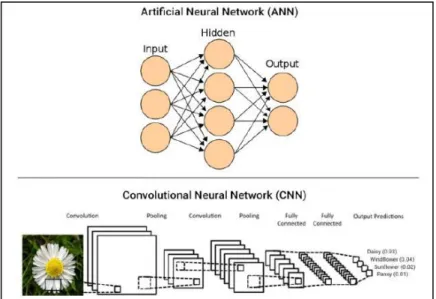
Figure 6 Artificial Neural Network (ANN) vs Convolutional Neural Network (CNN) Gogul & Kumar, 2017

11

2.5. B

ENCHMARK

D

ATASETS

In the past decade, face recognition was one of the research areas that has gained the most attention. Thanks to advances in hardware and efficient machine learning algorithms, it has made significant advances. Generally, machine learning relies on training computers with labelled data so that the characteristics of the data can have an impact on the overall performance of the system. In this respect, different benchmark datasets have been published. Although all datasets have collected frontal face images, each dataset has specific characteristics. The FERET dataset consists of a total of 14126 images of 1199 individuals, collected in a semi-controlled environment2_{. ORL contains a total} of 400 images of 40 individuals. The subjects appear in varyied lighting, at different times, facial expressions in eyes, smiling and, orientation(Abbas, Safi, & Rijab, 2017).

2_{https://www.nist.gov/programs-projects/face-recognition-technology-feret} Figure 7 Evolutionary history of deep CNNs (Khan et al. 2019)

12 Table 1 Available 2D face dataset (Aly & Hassaballah, 2015)

Name of database

Image

size #Images #Subject Colour/grey

Imaging

conditions Web address FERET 256 ×

384

14.126 1564 Colour controlled http://www.itl.nist.gov/iad/humanid/feret/feret_master.html

ORL 92 × 112

400 10 Grey Controlled http://www.cl.cam.ac.uk/research/dtg/facedatabase.html

AR 768 × 576 4 126 Colour Uncontrolled controlled http://www2.ece.ohiostate.edu/aleix/ARdatabase.html MIT-CBCL 115 × 115

2 10 Colour +3D models http://www.cbcl.mit.edu/heisele/facerecognition-database.html

SCface 4.16 130 Colour Uncontrolled http://www.scface.org/

Yale B 640 × 480

5.76 10 Grey Uncontrolled http://www.vision.ucsd.edu/leekc/ExtYaleDatabase/ExtYaleB.html

extended Yale B

640 × 480

16.128 28 Grey Uncontrolled http://www.vision.ucsd.edu/leekc/ExtYaleDatabase/ExtYaleB.html

CAS-PEAL 360 × 480 1704 × 2272 99.594 1.04 Grey Uncontrolled Controlled http://www.jdl.ac.cn/peal/index.html FRGC 1200 × 1600

12.776 688 Colour +3D models http://www.nist.gov/itl/iad/ig/frgc.cfm

FEI 640 × 480

2800 200 Colour Controlled http://www.fei.edu.br/cet/facedatabase.html

BioID 382 × 288

1.521 23 Grey Uncontrolled http://www.bioid.com/

MIW 154 125 Colour Uncontrolled http://www.antitza.com/makeup-datasets.html

CVL 640 × 480

114 7 Colour Uncontrolled http://www.lrv.fri.uni-lj.si/facedb.html

LFW 250 × 250

13.233 5.749 Colour Uncontrolled http://www.vis-www.cs.umass.edu/lfw/

LFW-a NIST (MID)

250 × 250

Colour uncontrolled http://www.openu.ac.il/home/hassner/data/lfwa/

1573 1573 Grey Controlled http://www.nist.gov/srd/nistsd18.cfm

KinFaceW 64 × 64 156, 134, 116 pairs of kinship Colour http://www.kinfacew.com/index.html NUAA PI 640 × 480

15 Colour anti-spoofing http://www.thatsmyface.com/

CASIA 640 × 480

50 Colour anti-spoofing http://www.cbsr.ia.ac.cn/english/FaceAntiSpoofDatabases.asp

Despite the datasets developed for different purposes, but none seem to have considered skin color and gender. Based on (Buolamwini, 2017) 79.6% - 86.24% of available face datasets are light skinned. IJB-A includes only 24.6% female and only 4.4% of them darker female, and 59.4% male with light skin. To address this issue, the PPB face dataset proposed 44.39% female and 47% dark skin.

13

2.6. F

ACE

R

ECOGNITION BIAS WITH DARK SKINS

Nowadays, we can clearly sense the existence of artificial intelligence in all part of society. From a simple software download for home applications, to a loan system or HR system to determining who should be hired in an organization and most importantly, assisting in determining how long someone should spend in prison - decisions traditionally made by humans (Buolamwini & Gebru, 2018). For years human society has been familiar with the fact that human life has been affected by technology but so far, the machines have never been decision-makers. Nowadays, AI-Based technologies can be trained to be used in a pipeline to perform high stakes tasks. Detroit police use face recognition technology to detect suspects. Thus, failure in the application can lead to serious consequences. Based on the NIST report, automated gender classification algorithms are more accurate for males than females (Ngan & Grother, 2015) and going beyond that Buolamwini and Gebru demonstrate that commercial face recognition algorithms have lower performance on dark-skin color than on white skin (Buolamwini & Gebru, 2018). Paper (Muthukumar et al., 2018) tried to find the reason behind this gap. They used an approximate PPB dataset with three classifiers. The first classifier is IBM Watson's gender classifier service, the second was IBM Watson deep-face-feature API that uses Support vector machine (SVM) with radial basis function (RBF) kernel and the third one was as same as second in term of SVM but used convolution neuron network (CNN) VGG and ResNet-50 as feature extractor. Unlike the previous report, surprisingly, the paper result will conclude to the point that skin type is not the driver. The paper suggests that lip and eye makeup are seen as strong predictors for a female face

2.7. A

PPLICATION

A

REA

As noted in the previous chapter, Face recognition is classified under biometric applications. Traditionally the applications in this group are associated with security sectors but nowadays, it expands to other industries such as retail, marketing in addition to the traditional field of security. Based on market-research web site report, facial recognition technology markets are estimated to reach $8.93 billion in revenue by the end of 2020, representing 3.3% of revenue for the entire IT market at that point in time3_.

According to papers (IJIS, 2019)(Chihaoui, Elkefi, Bellil, & Amar, 2009)(Meethongjan & Mohamad, 2007); face recognition can be used in two forms of identification and discovery for law enforcement. ▪ Identification; use to get confirmation of a subject face against the known face. For example, face recognition can help to confirm that does the subject is the same person as the face in the document presented such as passport, bank id, company badge or even hotel reservation. This approach is sometimes called one to one analysis.

▪ Discovery approach; helps to compare the subject face with numerous known faces. This approach, sometimes known as one to many analyses, is used in surveillance video tracking or still image and matching with a mug shot.

One of the most important sectors to which face recognition can be applied is healthcare. Using this technology in healthcare can enable doctors to monitor and diagnose certain diseases4_{. It results in}

14 earlier treatment which improve outcomes. Right now, few diseases and disorders can be detected, but with the advancement of this technology, this will increase.

In the context of face recognition applications for marketing, Forbes magazine published an article entitled “Facial Recognition Could Drive the Next Online Marketing Revolution: Here's How”. The author of the title stated that in the near future, using face recognition technology, in marketing would be more accurate and targeted. For example, it would be possible to identify consumer habits according to their facial expression, age, and gender, then show advertisements accordingly. In another example, retailers using this technology would be able to analyze their customers’ behaviors and based on the analysis adjust their retailing strategies.

Paper (Zhao et al., 2003), explained some application of face recognition in table 2. Table 2 Typical application area (Zhao, Chellappa, Phillips, & Rosenfeld, 2003)

Areas Specific Applications

Entertainment Video Game, Virtual reality, training programs

Human-robot-interaction, human-computer-interaction Smart cards

Drivers' licenses, entitlement programs

Immigration, national ID, passports, voter registration Welfare fraud

Information security

TV Parental control, personal device logon, desktop logon

Application security, database security, file encryption Intranet security, internet access, medical records Secure trading terminals

Law enforcement and surveillance

Advanced video surveillance, CCTV control Portal control, post event analysis

Shoplifting, suspect tracking and investigation

2.8. S

UMMARY

This chapter has been dedicated to face recognition literature review. We discussed the generic of face recognition and steps towards automated face recognition system.,We Also discussed different approaches and methods. Specifically, we reviewed the eigenface, LDA, ICA EBGM, HMM and finally different branches of neuron networks.

In the next chapter, we will discuss in more detail the algorithm and calculation part of each selected method.

15

3. METHODOLOGY

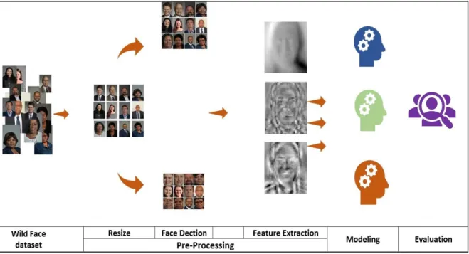
In this work, first, the Pilot Parliaments Benchmark (PPB) dataset was rebuilt and classified with 12 labels. Labels were defined based on VLS and Fitzpatrick methods. Then in the preprocessing phase, raw data (in this case images) was prepared for modeling. The support vector machine (SVM) method and CNN-ResNet152 were used as the classifier. Finally, results were evaluated with metrics. This work uses the confusion matrix for evaluation. Figure 8 shows the overall process for this paper.

3.1. D

ATA

C

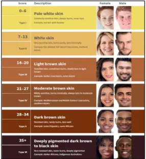
OLLECTION

Given the context of this paper, we used an approximate PPB data set. Approximate PPB face dataset consists of 1199 portrait of politicians from three African countries (South Africa, Senegal, Rwanda) and three European countries (Sweden, Finland, Iceland). The PPB was developed with the aim of a new benchmark with greater phenotype representation of skin type and gender(Buolamwini, 2017). To label the new benchmark face dataset, Joy Buolamwini used the Fitzpatrick method to differentiate interclass variation. Fitzpatrick is a method to describe and classify skin by reaction to exposure sunlight (Oakley, 2012). It is a numerical classification scheme that determines skin type based on the genetic constitution, reaction to sun and tanning habits. The response was measured on a scale of zero to four (Sachdeva, 2009).

Since determining Fitzpatrick scale needs to asses face reaction to the sun, just relying on this method is not rational. Hence this paper uses Von Luschan’s Chromatic Scale along with Fitzpatrick to fill the gap for skin reaction to the sun. Von Luschan's Chromatic Scale is the skin color classification, which can coordinate with the RGB system. This is the large color scale which covers 36 colors of human skin (Srimaharaj, Hemrungrote, & Chaisricharoen, 2016).

16 Figure 10 shows the 36-color scale of this method. To determine skin color in this paper, a database was developed that collects all visual information of each image, which is classified internally based Von Luschan's Chromatic Scale then used Fitzpatrick. Figure 9 shows the six levels of Fitzpatrick scale.

However, the original PPB was labelled with a binary construction of gender, but in this work, to explore more deeply 12 classes were used as labels that are based on gender and Fitzpatrick scale.

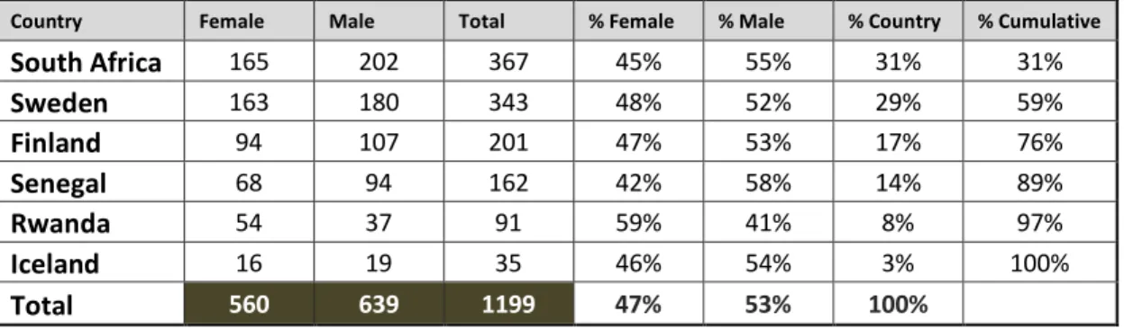
Approximate PPB contains 1199 portraits of politician from six countries that is fundamentally shaped with 47% female and 49% of dark skinned. Table 3. shows the basic information about approximate PPB.

Figure 10 Von Luschan's Chromatic Scale is a skin color classification, that use RGB system for classification.

VLC Scale (Srimaharaj, Hemrungrote, and Chaisricharoen 2016)

Figure 9 Fitzpatrick is a method to describe and classify skin by reaction to

exposure sunlight.

https://www.arpansa.gov.au/sites/defaul t/files/legacy/pubs/RadiationProtection/

17 Table 3 Face image distribution based on gender and country

Country Female Male Total % Female % Male % Country % Cumulative

South Africa 165 202 367 45% 55% 31% 31% Sweden 163 180 343 48% 52% 29% 59% Finland 94 107 201 47% 53% 17% 76% Senegal 68 94 162 42% 58% 14% 89% Rwanda 54 37 91 59% 41% 8% 97% Iceland 16 19 35 46% 54% 3% 100% Total 560 639 1199 47% 53% 100%

Table 4. show the distribution based on skin type. Table 4 Skin type distribution

Country Type I Type II Type III Type IV Type V Type VI

Finland 23% 57% 19% 0% 0% 0% Iceland 0% 49% 49% 3% 0% 0% Rwanda 0% 0% 1% 3% 65% 31% Senegal 0% 0% 0% 4% 22% 75% South Africa 2% 6% 5% 7% 37% 43% Sweden 34% 48% 14% 3% 1% 1%

South Africa with 367 records has the highest number of images and Iceland with 35 images has the lowest number of records. However, the dataset is almost balanced in relation to gender type (47% Female and 53% male) overall (see table 3) but interclass gender distribution is shown somewhat inconsistent for skin types 5 and 6. Figure. 11 shows a comparison between classes. The dataset contains 202 males versus 109 females in skin type 6 that the male population is almost double that of females while in skin type 5 is the opposite. Most of this inconsistency comes from Senegal and South Africa data, where the majority of females are classified under skin type 6 but most males are classified under type 5. Three countries (South Africa, Sweden, and Finland) comprise 76% of the total population but overall there is a balance between the number of dark skin images and light skin images, as shown in table 3. It is worth mentioning that Finland is the only country in the list with a pure population of light skin and Senegal is the only country with a pure population of dark skin.

Figure 11 Gender population based on skin type (project work)

18

3.2. S

OFTWARE AND

L

IBRARIES

In this work, python 3 was used as the programming language tool to run the code and to determine skin color label for each face image, I used Microsoft Access. Microsoft Access is a desktop application from Microsoft office package. It is a useful tool to compare skin color with two standard scale and store its data.

Along with these tools, various machine learning libraries were used, as described below: ▪ Matplotlib

Matplotlib is a Python 2D plotting library which produces publication quality figures in a variety of hardcopy formats and interactive environments across platforms5_.

▪ OpenCV

OpenCV (Open Source Computer Vision Library) is an open source computer vision and machine learning software library. OpenCV was built to provide a common infrastructure for computer vision applications and to accelerate the use of machine perception in the commercial products6_.

▪ Sklearn

Scikit-learn (formerly scikits.learn and also known as sklearn) is a free software machine learning library for the Python programming language. It features various classification, regression and clustering algorithms including support vector machines, random forests, gradient boosting, k-means and DBSCAN, and is designed to interoperate with the Python numerical and scientific libraries NumPy and SciPy7_.

▪ Keras

Keras is an open-source neural-network library written in Python. It is capable of running on top of TensorFlow, Microsoft Cognitive Toolkit, R, Theano, or PlaidML. Designed to enable fast experimentation with deep neural networks8_.

3.3. P

RE

-P

ROCESSING

Preprocessing is a fundamental part of any type of data processing. This principle also applies to face recognition as one type of data processing. Image preprocessing applies with aims to reduce noise, contrast enhancement, and image smoothing(Adatrao & Mittal, 2016).

This paper applied the following steps to prepare raw images for processing: 1. Load Raw Data

This step is an initial part of image processing. As python is a script programming language, the image should be transformed to number, so images convert to the matrix using by OpenCV library. The output of this step is a list of a 3-dimensional matrix.

2. Convert to Gray Scale

In grayscale images, the value for each pixel is representing only the amount of light9_{. With a} simple query on the internet, it is easy to find out that there are many supporters and

5 _{Matplotlib official websit: https://matplotlib.org/index.html} 6 _{OpenCV official websit: https://opencv.org/about/}

7 _{Wikipedia: https://en.wikipedia.org/wiki/Scikit-learn} 8 _{Wikipedia: https://en.wikipedia.org/wiki/Keras}

19 detractors regarding image processing in grayscale mode. Based on the context of this paper, both gray and colored data are ketp for processing.

3. Resize images to “500 × 300”

Since the images were gathered from different sources, there were several sizes that were a cause of inconsistency in the dataset. Thus, this step resizes all images to a new size scale. In another word, all images size change to 500 height and 300 weight pixels.

4. Crop Image to “only faces” and “face with hair”

As recognition is based on faces, background data is useless for the process. To reduce dimensionality and enhance accuracy, the face will be detected and cropped. Based on the objective of this work, we generated two new data sets that store cropped face based on two modes “only faces” and “face with hair”

5. Convert image list to matrix

as the final step, the images were reshaped to flat and embedded into a matrix. This matrix is represented by the image dataset so that each row represents an image and the columns represent image features.

3.4. M

ODELING

As mentioned in section 2.4 It seems that there is no certainty in method selection. We can see in the evolution of face recognition methods, it would be better if we compare it based on approach and method. Hence, in this work, we selected three methods based on two criteria; popularity in the approach class and simplicity. Based on the criteria, the three methods selected are the following: ▪ Eigenface

▪ Independent Component Analysis (ICA) ▪ CNN

9_{https://en.wikipedia.org/wiki/Grayscale}

Figure 12 Convert RGB color to grayscale image (PPB dataset)

20

3.4.1. Eigenface

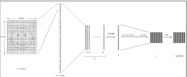
Eigenface is a well-known statistical method based PCA that is used for dimensional reduction. Sirovich and Kirby used this method for the first time to represent face image. Later Turk and Pentland employed the technique for face recognition. Although the technique works well with a smaller number of images the performance will decrease in high dimensions space (Vanlalhruaia et al., 2015). In this method, images are decomposed to sets of eigenfaces and reconstructed by adding a weight called eigenvalue. The following steps describe this mathematically.

1. Adapt the matrix 𝐼i into a vector

This step is, in fact, the last step of pre-processing. The matrix will convert to a vector that has lower-dimensional space than the matrix. We will convert the matrix to a vector so that each vector represent a facial image. From now on, all calculation will apply on vectors.

2. Calculate the average value of the vectors

To obtain the average vector, after summing all vectors ( ) divide it by the total number of images (M). formula (1), represents average vectors and represent images vectors.

(1)

3. Obtain by subtracting the average value from the vector

To have a representative vector that can like a batch for an image, we will subtract each vector from the average vector. Each image represented by a new vector . From now on we will work with a new representative set “average face” A= [ ]

(2)

Figure 13 Convert Matrix to Vector

21 4. Compute the covariance matrix C

Covariance matrix used to calculate the variation among multiple faces(Zafaruddin & Fadewar, 2014). Covariance matrix C is computed based on multiplying matrix A with its transposition AT. Matrix A is, in fact, the images matrix that subtracted the mean . Figure 14 shows the process of producing covariance matrix C.

(3)

5. Compute eigenvalue and eigenvectors

As it is obvious, working with a small number of features is much easier and more manageable than working with the whole set. On the other hand, a small set or even a scalar value of matrix can have a huge effect on final recognition. In this step PCA technique is applied on average face set to reduce the dimensionality while try to avoid losing valuable information. The output of PCA would be Principal Component Analysis thatis called Eigenface. Follow equation (4) use to extract Eigenvalues that is the weight to reconstruct the face. In the formula (4), A is the matrix, 𝜆 is the eigenvalue and I is the identity matrix.

(4)

To extract 𝜆, formula(5) uses to calculating the determinant

(5)

Figure 14 Covariance matrix C

22 6. Selecting K best Component and Face Recognition

In this step, Best K eigenvector/eigenface will be selected. Each K is a training set representation in the form of a linear combination. Typically vectors with the highest eigenvalue would be selected. Recognition will be done by using the Euclidean or Mahalanobis method for measuring the distance to find a match of the face image.

3.4.2. Independet Componant Analysis (ICA)

Independent Component Analysis (ICA) is a statistical method for face recognition. The goal for ICA is to decompose an observed image into a linear combination of the unknown independent component by minimizing statistical dependency between the component (Toygar & Introduction, 2003)(Draper, Baek, Bartlett, & Beveridge, 2003). Same as PCA, perform by dimension reduction and feature extraction but unlike it, its high order dependency in addition to removing correlation among the data.

ICA is intimately related to blind source separation (BSS) that is associated with the extraction of source signals from sets of mixed signals and it is also a well-known solution for the cocktail party problem. This problem requires to separate mixed sounds in the cocktail party to origins of each. So far, several algorithms proposed based on ICA, such as Fast ICA, Algebraic ICA, Tensor Based ICA, Infomax Estimation (Acharya & Panda, 2008).

In a simple scenario, we have observed data (mixtures) represented by a random vector

and we another set as random source vector

.

The task for ICA is to transform observed data by using linear statistic transformation as into an observable vector of maximally independent components s.

In ICA there are three assumption to solve the problem ▪ Mixing process is liner

▪ All sources are independent

▪ All sources have none-gaussian distribution

Mathematically assume, N mixture from N independent component. Follow equation (6) formulate mix signal. is mix signal, a is mixing cofficient is source signal

23

(6)

therefore, by using the coefficients the source linearly transformed from S to mixed signal in X space as follow(Tharwat, 2018).

(7)

To extract independent component based on the assumption ICA algorithm try to find mix matrix A that u is an independent component, W is weight or unmixing coefficient and x is the mixed matrix(Tharwat, 2018).

(8)

As ICA assumes that observed data x are a linear combination of independent component Whitening transform is required to decorrelation and uniform. Whitening transform can be determined as where D is a diagonal matrix of the eigenvalue and R is the matrix of orthogonal eigenvector (Draper et al., 2003).

24

3.4.3. Convolutional neural network (CNN) – ResNet152

Convolution Neural Network (CNN) is a class of artificial neural networks. CNNs is popular for processing data with a grid pattern (Yamashita, Nishio, Do, & Togashi, 2018). Same as neural network architecture, automatic learning and adaptation happen through backpropagation in the different building blocks. CNNs is composed of multiple building blocks such as “convolution layer”, “pooling layer” and “fully connection layer”. Figure 18 shows the overall structure for CNN. The first two layers are feature extraction and the third one, fully connected layer used for mapping and classification.

▪ Convolution layer

This is one of the fundamental components of CNNs architecture. This layer is used for feature extraction where a small array of numbers called kernel, applied across the input, which is an array of numbers called tensor. Each kernel can be considered as a different feature extractor or filter, typically is with size 3×3 but sometimes it is 5×5 or 7×7(Yamashita et al., 2018). Elementwise the kernel multiplied by mapped input tensor and summed to obtain output value for the corresponding location. Repeatedly this process applied to the arbitrary number of features mapped from input tensor. The arbitrary number is correlated with a stride parameter. Stride is the number that specifies the length of the convolution kernel jump. As much as stride number is bigger, kernel movement is faster but there is less overlap. In addition to kernel size and stride, there is one more parameter in the convolution

Figure 18 An overview of a convolutional neural network (CNN) architecture and the training process. (Yamashita, Nishio, Do, & Togashi, 2018)

Figure 19 Convolution layer

25 layer called “padding”.

As of the last operation in the convolution layer, an activation function will apply to compute the linearity output of the convolution layer to a nonlinearity. Although sigmoid, hyperbolic and tangent functions are popular activation functions in the neural network but rectified linear unit (ReLU) is so common in CNNs. The ReLU layer applies the function f(x) = Max (0, x) to all the values in the input volume. In basic terms, this layer just changes all the negative activations to 0. This layer increases the nonlinear properties of the model and the overall network without affecting the receptive fields of the Conv layer.

▪ Padding

As mentioned, padding is an additional parameter: rows and columns of zeros are added on each side of the input tensor. The main objective of add padding is to provide more overlap with center elements of the kernel and outermost element of the tensor. Also, it helps to avoid loss of information and unwanted size reduction.

▪ Pooling layer

This layer provides a down-sampling operation. Normally it helps to reduce the dimensionality of features. Reference (Boureau, Ponce, Fr, & Lecun, 2010) describe two types of pooling layer; Max pooling and average pooling. Although average pooling was used historically,recently max pooling performs better. Although there is no pre agreed size for pooling, typically a filter size of 2×2 and stride 2 is popular. However, choosing a large filter can significantly reduce the input dimensionality and loss of information.

Figure 20 Padding https://becominghuman.ai/

how-should-i-start-with-cnn-c62a3a89493b

26 Max pooling extract patches based on filter size and stride parameter from the input feature and return the maximum value of each patch.

▪ Fully connected layer

Eventually, a fully connected layer is the last layer of CNNs, also known as dense layer. Typically, a fully connected layer has output, the same number of classes. The output feature from pooling or Conv layers will transform into a flatted layer (1-dimension array or vector) and then mapped by a subset of the fully connected layer. In the final stage, there is a competitive process with the probability of each class. In simple words, once features extracted by convolution layers and down-sampled by pooling, as the last step, it will be mapped and ranked by a fully connected layer(Yamashita et al., 2018).

3.4.3.1. ResNet Architecture

ResNet was proposed by Kaiming He et al. This concept revolutionized the CNN architectural race by introducing the concept of residual learning in CNNs(Khan et al., 2019).

Based on figure 22, ResNet function, duplicate the given input to keep the previous output from possible bad transformation.

Based on structure, once the original value of Y stored, it undertakes some process of convolution operation to maximize the learning. As the original Y already stored, it added with the transformed Y.

Figure 22 ResNet Bock prevent from bad transformation by keeping input https://towardsdatascience.com/introduc

27 Figure 23 ResNet-152 vs

VGG-19 (Han et al., 2018)

This skip process helps to avoid elimination of possible negative effects in transformation. Figure. 23 shows the overall schematic structure ResNet152 and VGG-19.

3.5. E

VALUATION

To evaluate and compare the result, this work uses the confusion matrix. Confusion matrix is one of the easiest and most intuitive tool for classification problems. It is a N×N matrix that N represents the number of classes being predicts (in this case N=12)[183]. Figure 24 shows a sample format of the confusion matrix.

Following are some measures of the confusion matrix that was published by (Srivastava, 2019). Accuracy : the proportion of the total number of predictions that were correct. (9)

(9)

Figure 24 Confusion matrix is one of the easiest and

28 Precision : the proportion of positive cases that were correctly identified. (10)

(10)

Sensitivity or Recall : the proportion of actual positive cases which are correctly identified. (11)

(11)

Specificity : the proportion of actual negative cases which are correctly identified. ()

(12)

F1-score : it is a classifier metric that calculates mean of precision and recall. Somehow it is weight of a class that emphasizes to lowest value. F1-score is a metric to ensure that both parameter recall and precision is indicating a good result.

(13)

In simple terms, high precision means that an algorithm returns substantially more relevant results than irrelevant ones, while high recall means that an algorithm returns most of the relevant results10_. To evaluate models, this work mainly tracks precision, recall, and F1-score

29

4. RESULTS AND DISCUSSION

4.1. E

IGENFACE

R

ESULT

The eigenface method is based on PCA dimension reduction. This work uses this method as a base method. As mentioned in section 3.1, the experiment uses 1199 images (965 train set and 234 test set). The test was conducted in two cycles with two types of data set, “only face” and “face with hair” data set.

In the first cycle, the model tested with “only face” data set. The data set contain images that cropped face from original with size 36×36 pixel. All images were converted to grayscale. Overall, the model achieved 63% accuracy with 400 principal components. The number of principal components selected was based on the maximum variation amount. Figure 25 shows the variation curve. Theoretically, when gradient descent starts to approach zero, it has the maximum variation. In other words, the number of components at this point has the best representative.

Based on test result class label F_TY_VI that represents females with skin type 6 had the highest rate of correct prediction (45%) that is so called recall. Put simply word recall is the ratio of total predictive positive classes divided by the total number of predict positive that is simply the sensitivity, so in our case, high sensitivity is our preference. In the second and third class label, M_TY_II and F_TY_II with recall rate 34.4% and 30.3% had the highest rate respectively. On the opposite side, class labels F_TY_IV and M_TY_IV are the lowest recall (0%). Table 5 shows the result of the classification report.

Figure 11 shows that F_TY_VI has 109 records which surprisingly is not the largest number of records in the data set but M_TY_II and F_TY_II are the second and third populate groups in the dataset. Also, F_TY_IV and M_TY_IV have the lowest rate. Moreover, these class labels have the lowest number of records in the dataset.

If we ignore the first result, we can conclude that there is a positive correlation between the number of trained data in each class and the true positive predict rate in the eigenface method.