EUROPEAN ORGANIZATION FOR NUCLEAR RESEARCH (CERN)
CERN-EP/2016-320 2017/01/10
CMS-TRK-15-002
Mechanical stability of the CMS strip tracker measured
with a laser alignment system
The CMS Collaboration
∗Abstract
The CMS tracker consists of 206 m2of silicon strip sensors assembled on carbon fibre
composite structures and is designed for operation in the temperature range from−25
to +25◦C. The mechanical stability of tracker components during physics operation
was monitored with a few µm resolution using a dedicated laser alignment system as well as particle tracks from cosmic rays and hadron-hadron collisions. During the LHC operational period of 2011–2013 at stable temperatures, the components of the tracker were observed to experience relative movements of less than 30 µm. In addi-tion, temperature variations were found to cause displacements of tracker structures
of about 2 µm/◦C, which largely revert to their initial positions when the temperature
is restored to its original value.
Submitted to the Journal of Instrumentation
c
2017 CERN for the benefit of the CMS Collaboration. CC-BY-3.0 license ∗See Appendix A for the list of collaboration members
arXiv:1701.02022v1 [physics.ins-det] 8 Jan 2017
1
1
Introduction
The silicon strip tracker of the CMS experiment at the CERN LHC is designed to provide precise and efficient measurements of charged particle trajectories in a solenoidal magnetic field of 3.8 T with a transverse momentum accuracy of 1–10% in the range of 1–1000 GeV/c in the central region [1]. It consists of five main subdetectors: the tracker inner barrel with inner disks (TIB and TID), the tracker outer barrel (TOB), and the tracker endcaps on positive and negative sides (TECP and TECM) [2, 3]. The silicon strip sensors have pitches varying from 80 µm at the innermost radial position of 20 cm, to 205 µm at the outermost radius of 116 cm, delivering a single-hit resolution between 10 and 50 µm [1]. As a general criterion, the position of the silicon modules has to be known to much better accuracy than this intrinsic resolution.
Silicon sensors exposed to a large radiation fluence require cooling, and the CMS tracker is
de-signed to operate in a wide temperature range from−25 to+25◦C. The mechanical stability of
the tracker components is ensured by the choice of materials and by an engineering design that tolerates the expected thermal expansion and detector displacements. These displacements have to be measured and accounted for in the form of alignment constants used in the track reconstruction.
The absolute alignment of individual silicon modules is performed with cosmic ray muons and tracks from hadron-hadron collisions collected during periods of commissioning or col-lision data taking [4–6]. A significant advance in the track-based alignment came with the
introduction of a global χ2algorithm that combines reconstruction of the track and alignment
parameters [7]. This algorithm, implemented in theMILLEPEDE package [8], was successfully
used in various experiments at the LHC, HERA, and Tevatron. The actual accuracy of the track-based alignment depends on the number of objects requiring alignment and the size of the track sample.
The movement of the tracker components over much shorter time scales is monitored in the CMS experiment with an optical laser alignment system (LAS) [9]. Lasers were already used in the alignment of several silicon-based tracking detectors, for example, in the ALEPH [10], ZEUS [11], and AMS02 [12] experiments. Moreover, the CMS experiment also uses lasers for linking the tracker and muon subdetectors together in a common reference frame [13]. There is an alternative method of optical alignment based on the RasNiK system that was implemented, for example, in the CDF [14] and ATLAS [15] experiments. The RasNik system uses a conven-tional light source with coded mask, a lens, and a dedicated optical sensor. Both methods have similar performance, but lasers have some advantages for operation in the CMS tracker. First, the infrared laser light penetrates the silicon sensors, hence simplifying the alignment system. Second, the laser light produces a signal similar to ionizing particles that permits the use of the same radiation-hard silicon detectors employed for tracking, instead of dedicated sensors. The LAS of the CMS tracker is one of the largest laser-based alignment systems ever built in high-energy physics. Forty infrared laser beams illuminate a subset of 449 silicon modules, and monitor relative displacements of the TIB, TOB, and TEC subdetectors over a time interval of a few minutes with a stability of a few µm [9]. Alignment with particle tracks and laser beams are complementary techniques and together they ensure the high quality of track reconstruc-tion.
In this paper we describe the mechanical structure of the tracker and the LAS in detail. We review the alignment procedure of using laser beams and particle tracks. The measurements of the mechanical stability of the tracker components during the LHC data taking period in 2011– 2013, as well as during the LHC long shutdown period spanning 2013–2014, are presented and discussed.
2 2 Mechanical design of the CMS tracker 9/21/16 1 EC AL y x z Δx Rz Ry Rx Δy +x +z
Tracker support bracket Tracker support tube Tracker bulkhead TECM TECP TOB pixel TIB TIB TID TID ECAL Δz
Figure 1: Mechanical layout and mounting of the tracker subdetectors (bottom half is shown). The TIB+TID are mounted inside the TOB, while the TOB, TECP, and the TECM are mounted inside the TST. The red arrows indicate the connection points and their kinematic constraints.
2
Mechanical design of the CMS tracker
The silicon strip tracker of the CMS detector is composed of 15 148 silicon strip detector
mod-ules with a total area of about 206 m2and is described in Refs. [2, 3]. Below we discuss in more
detail the components of the tracker that are relevant to the mechanical stability of the detec-tor. The mechanical concept of the tracker is sketched in Figure 1. The CMS coordinate system has its origin at the centre of the detector with the z-coordinate along the LHC beam pipe, in the direction of the counterclockwise proton beam, and the horizontal x- and the vertical y-coordinates perpendicular to the beam (in the cylindrical system r is the radial distance and ϕ is the azimuth). The inner radii from 4.4 up to 15 cm are occupied by the silicon pixel detector, which is operated independently of the strip tracker. The silicon strip modules are mounted around the beam pipe at radii from 20 cm to 116 cm inside a cylinder of 2.4 m in diameter and
5.6 m in length. The TIB extends in z to±70 cm and in radius to 55 cm. It is composed of two
half-length barrels with four detector layers, supplemented by three TID disks at each end. The TID disks are equipped with wedge-shaped silicon detectors with radial strips. The TOB
sur-rounds the TIB+TID. It has an outer radius of 116 cm, ranges in|z|up to 118 cm, and consists
of six barrel layers. In the barrel part of the tracker, the detector strips are oriented along the z-direction, except for the double-sided stereo modules in the first two layers of the TIB and TOB, where they are rotated at an angle of 100 mrad, providing reconstruction of the z-coordinate.
The TECP and TECM cover the region 124 < |z| < 282 cm and 22.5 < r < 113.5 cm. Each
TEC is composed of nine disks, carrying up to seven rings of wedge-shaped silicon detectors with radial strips, similar to TID. Rings 1, 2, and 5 are also equipped with stereo modules for
3
reconstruction of the r-coordinate.
Each module of the silicon strip detector has one or two silicon sensors that are glued on carbon fibre (CF) frames together with a ceramic readout hybrid, with a mounting precision of 10 µm. Overall, there are 27 different module designs optimized for different positions in the tracker. The detector modules are mounted on substructures that are, in turn, mounted on the tracker subdetectors.
The TIB is split into two halves for the negative and positive z-coordinates allowing easy inser-tion into the TOB. The TIB substructures consist of 16 CF half-cylinders, or shells. The mount-ing accuracy of detector modules on the shells is about 20 µm. The modules are assembled in rows that overlap like roof tiles for better coverage and compensation for the Lorentz angle [3].
An aluminium cooling tube, with 0.3 mm wall thickness and 4×1.5 mm2 rectangular profile is
glued to the mounts of the detector modules. Each row has three modules on one cooling loop and each cooling pipe is connected at the edges of the shells to the circular collector pipe that gives extra rigidity to the whole TIB mechanical structure. The overall positional accuracy of the assembly of all shells is about 500 µm.
The TOB main structure consists of six cylindrical layers supported by four disks, two at the ends and two in the middle of the TOB structure. The disks are made of 2 mm thick CF laminate and are connected by cylinders at the inner and outer diameters. The cylinders are produced from 0.4 mm CF skins glued onto two sides of a 20 mm thick aramid-fibre honeycomb core. The detector modules are mounted on 688 substructures called rods. The rods are inserted into openings on the disks, such that each rod is supported by two disks. The accuracy of mounting the rods is about 140 µm in r-ϕ and 500 µm in z. Each rod has 6 or 12 (for rods with double-sided modules) silicon modules mounted in a row. A 2 mm diameter copper-nickel cooling pipe is attached to the CF frame of the rod. Each module is mounted on the rod with an accuracy of 30 µm by two precision inserts connected to cooling pipes and two springs.
Each TEC side consists of nine disks with 16 wedge-shaped substructures on each disk, called petals. Overall there are 144 petals with different layouts, depending on the disk location. The petals are made of CF skins with a honeycomb structure inside. The wedge-shaped detector modules are mounted on the petals with an accuracy of 20 µm using four aluminium inserts that are connected to the cooling pipe. A titanium cooling pipe of about 7 m in length, 3.9 mm in diameter, with 0.25 mm wall thickness is integrated into the petal honeycomb structure and is bent to connect all heat sink inserts. The petals are mounted on the CF disks with a precision of 70 µm. All nine disks of each TEC are connected together with eight CF bars forming a rigid structure. These bars are also used to hold service cables and cooling pipes. The overall accuracy of the disk assembly is about 150 µm.
The main support structure for all tracker subdetectors is the tracker support tube (TST). The TST is a cylinder 5.4 m in length and 2.4 m in diameter made of CF composite. The wall of the TST is made of a 30 mm thick sandwich structure with 2 mm CF skins on both sides, and a 26 mm thick aluminium honeycomb core. The TOB, TECP, and the TECM are supported inside the TST while the TIB and TID are supported by the TOB. The total weight of all subdetectors inside the TST is about 2200 kg, which is distributed on two longitudinal rails connected to the TST with glue and metallic inserts. The TST itself is supported inside the CMS calorimeters by four brackets at each end. According to calculations the maximum deformation of the TST when supporting the assembled tracker is about 0.6 mm. The mounting accuracy of different subdetectors inside the TST is in the range of 1 mm, but the exact position of all subdetectors was measured with an accuracy of 50 µm in an optical survey conducted at the beginning of the detector operation [5].
4 2 Mechanical design of the CMS tracker
The detector modules, substructures, and subdetectors are joined together using the so-called kinematic connections that constrain the movement in some directions, where the constraints are ensured by the static friction in tension screws. The engineering designs of these connec-tions in the various mechanical structures are different, but the range in all joints suffices to accommodate the expected thermal expansion. The fixation points and allowable movements for the subdetectors are indicated in Figure 1. In the vertical direction, each subdetector is con-strained only by its own weight. The movement in the x-direction is concon-strained only on one side of the TST. The fixations in the z-coordinate are governed by the assembly procedure. Dur-ing the assembly, the TOB was first inserted into the TST and fixed in z on one side. Then the TIB and TID halves were inserted into the TOB from each end and fixed against each other in the centre. The TECP and TECM were mounted last, and constrained in z at the internal ends. Operation of silicon modules exposed to a large radiation fluence requires cooling [3]. The total dissipated power of the readout electronics with a fully powered tracker is about 45 kW. After irradiation the leakage current of the silicon sensors contributes another 10 kW. The heat inside
the tracker is evacuated by a monophase liquid-cooling system that uses a fluorocarbon (C6F14)
coolant. Two cooling plants, each with 40 kW capacity, are used for this purpose. Each plant is connected to 90 cooling loops distributed among the different substructures in one half of the tracker.
The low-temperature operation also requires a low dew point inside the tracker. The whole tracker volume is separated from the TST inner wall by a thermal screen, apart from the points at which the subdetectors are attached to the rails that remain at ambient temperature. The thermal screen has cooling elements inside and heating elements outside the tracker volume,
thus acting as a thermal barrier. The inner tracker volume of about 25 m3is constantly flushed
with dry air or nitrogen at a rate of about 20 m3/hour, such that the dew point in the CMS
cavern of about+10◦C is reduced to below−40◦C inside the tracker volume. All service cables
and cooling pipes leave the subsystem at the tracker bulkheads, which are also isolated by the
thermal screen and flushed with dry gas at a higher rate of about 150 m3/hour.
In the first physics run during 2010–2013 (Run 1), the operating temperature of the cooling
plant was set to T= +4◦C. For Run 2 (2015 onwards), the nominal operating temperature was
decreased to −15◦C, in order to allow operation with increased fluence caused by increased
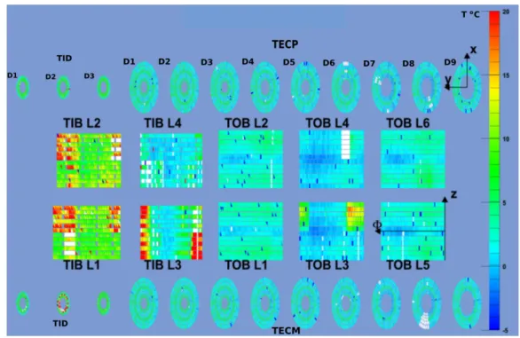
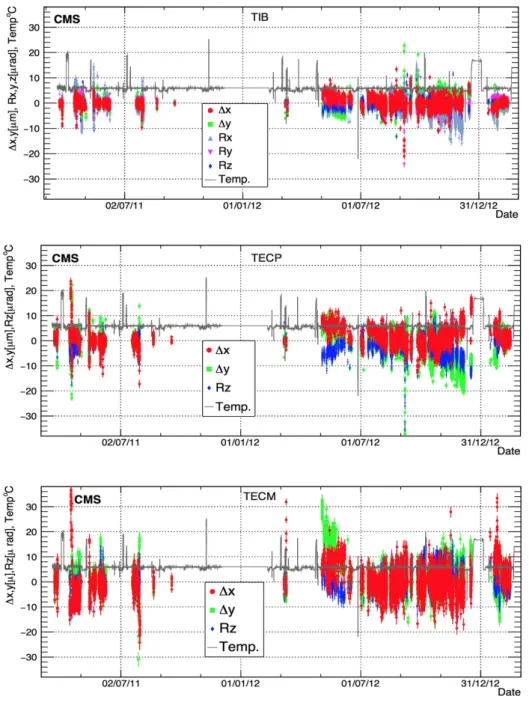
energy of collisions, as well as instantaneous luminosity [3]. The temperature of the differ-ent mechanical structures inside the tracker depends on the distribution of heat sources and heat sinks. The temperature and humidity inside the tracker are monitored by dedicated sen-sors mounted directly on readout hybrids, silicon sensen-sors, mechanical structures, distributed throughout the detector volume. The nonuniformity of heat dissipation and evacuation results in significant temperature variations inside the tracker even in thermal equilibrium. Large tem-perature gradients are observed near the readout hybrids, the cooling tubes and the mounting connections. Figure 2 shows the temperature measured on silicon sensors in different
subdetec-tors running with a cooling plant at operating temperature of−5◦C. The white areas represent
non-operational detectors, which comprise about 2.5% of the total area. The red (hot) spots are the five cooling loops (three in the TIB, and one in the TOB and the TID) that are closed because of leaks and degraded cooling contacts (layers L1, and L2 in the TIB).
A local change of temperature naturally causes an increase in the nonuniformity. For exam-ple, the powering of the module readout electronics rapidly increases the local temperature
by about 15◦C and it takes about one hour to stabilize the temperature in the tracker volume.
Cooling down from the ambient temperature of about +15◦C to +4◦C takes about 3 hours
5
Figure 2: Example of the temperature distribution, shown as a colour palette (◦C), measured
on silicon sensors in the TIB (L1–L4), TOB layers (L1–L6), and the TEC (D1–D9), TID (D1–D3)
disks, with the cooling plant operating at T= −5◦C. The white spots correspond to
nonopera-tional detectors, and red spots are the closed cooling loops and bad cooling contacts.
3
The laser alignment system
The initial purpose of the LAS was to measure relative positions of the tracker with an accuracy of about 10 µm and the absolute position with an accuracy of 100 µm. The large temperature variations expected in the tracker determined the design concept and components for the LAS; the components had to be light, radiation hard, operational in a high magnetic field, and capa-ble of sustaining large temperature variations.
The LAS has 40 infrared laser beams that illuminate the silicon strip modules in the outer layer of the TIB, inner layer of the TOB, and in rings 4 and 6 of the TECs, as shown in Figure 3. The LAS uses the same detector modules that are used for particle detection. Laser pulses are triggered during the 3 µs orbit gap corresponding to 119 missing bunches in the LHC beam structure that has an orbit time of 89 s, thus not interfering with collisions [2]. The laser beams are split into two sets. Eight beams are used for global alignment of the TIB, TOB, and the TECs relative to each other. The other 32 beams are used to internally align the disks in the TECP and TECM subdetectors. The pixel and the TID subdetectors are not included in the LAS monitoring. Since the tracker has approximate axial symmetry, the beams are distributed rather uniformly in the ϕ-direction, with the exact position defined by the mechanical layout. Each laser beam used for global alignment illuminates six modules in the TIB, six modules in the TOB, and five modules in each of the TECP and TECM subdetectors. Each laser beam for the internal TEC alignment traverses nine modules in each TEC subdetector.
The LAS components include laser diodes, depolarizers, optical fibres, beam splitters, align-ment tubes, mirrors, and specially treated silicon sensors. The laser diodes QFLD-1060-50S
6 3 The laser alignment system pixel TOB TECP TECM TIB from lasers TID laser beam beam splitter alignment tube optical fibre
Figure 3: Distribution of the laser beams in the CMS tracker. The eight laser beams inside the alignment tubes are used for the global alignment of TOB, TIB, and TEC subdetectors. The 32 laser beams in the TECs are used for the internal alignment of TEC disks.
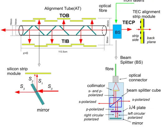
Beam Splitter (BS) 16 m m 14 m m 36 m m 50m m 113.5cm z=0 TECP TIB optical fibre TOB from lasers silicon strip module mirror S1 S2 collimator λ/4 plate s-polarized s-polarized p-polarized optical connector fibre
beam splitter cube
mirror right circular polarized S0 S3 left circular polarized BS s- and p-polarized Alignment Tube(AT) TEC alignment strip module back plane strip side
Figure 4: The LAS components: alignment tube, mirror, and beam splitter.
power of 50 mW. The attenuation length of this laser light in silicon is 10 cm at 0◦C and
de-creases by 1%/◦C with increasing temperature. The light output of each laser is regulated by
7
operate in pulsed mode with a pulse width of 50 ns. The spectral bandwidth of the lasers is
∆λ = 2.4±0.9 nm, which defines the coherence length λ2/∆λ ≈ 480 µm. A coherence length
larger than 2d·nSi (where d is the silicon thickness of 320–500 µm and nSi ≈ 3.5 is the
sili-con refractive index) would result in interference of the laser light reflected on the front- and back-side of the sensor, hence degrading the laser beam profile. Because of the harsh radiation conditions in the CMS detector cavern, the laser diodes are located in the outer underground service area. The light is distributed to different subdetectors via special 0.125 mm diameter Corning monomode optical fibres.
The light from the lasers is directed towards different subdetectors using beam splitters (BS) that divide the light into back-to-back beams, as shown in Figure 3. For the global alignment the eight beam splitters for the eight laser beams are mounted between the TOB and TECP. For the internal TEC alignment, 32 BS are located on disk 6 in both TECP and TECM. The principle of operation of the beam splitter is based on polarization using a λ-plate, as shown in Figure 4. The incoming beam, consisting of both s- (perpendicular to the plane of incidence) and
p-(parallel) polarizations, is collimated onto a 45◦ inclined surface with a special coating, from
which the s-polarized part of the laser light is completely reflected. The p-fraction continues, traversing a λ/4-plate and converting into right circular polarization. The light is reflected by a mirror after the plate and changes polarization to left circular. After a second traversal of the
λ/4-plate, the left circularly polarized light becomes s-polarized and is completely reflected
onto the other side of the 45◦ inclined surface. At the end, there are two parallel back-to-back
beams with s-polarization in the z-direction. The important characteristic of the splitter is the variation of collinearity as a function of the beam spot position. For all BS, the collinearity is
measured to be less than 50 µrad for the−25 to+25◦C temperature range. Since the laser light
is polarized, splitting based on a λ-plate requires depolarization. The depolarizers (produced by Phoenix Photonics) are located in the service area just after the laser diodes and before the optical fibres.
Dedicated alignment tubes (AT) between the TIB and TOB are used to hold the BS and semi-transparent mirrors that reflect light towards TOB and TIB detector modules, as shown in Fig-ure 4. The eight laser beams between TOB and TIB pass through the AT and continue to the TECM disks. The AT are made from 16 mm diameter aluminium and are integrated into the TOB support wheels. The mirrors mounted inside the AT are glass plates that reflect about 5%
of the light intensity perpendicular to the beam (S1). The antireflective coating on the back side
of the mirror and the s-polarization of the laser light after the beam splitter prevent the second
reflection (S2). The mounting accuracy of each AT is about 100 µm, but with temperature
vari-ations the aluminium can expand by about 0.5 mm/20◦C. Although this expansion is mostly
along the z-direction, the movement can affect the orientation of the BS and therefore the di-rection of the laser beams. Such variations are taken into account in the LAS reconstruction procedure, as discussed below.
Overall the laser beams hit 449 silicon sensors, with a strip pitch varying from 120 µm in the TIB to 156 µm in the TEC detector modules. The 48 TIB and 48 TOB sensors that are used by the LAS are standard ones, and are illuminated on the strip side. On the other hand, 353 TEC sensors had to be modified to allow the passage of laser light. For the standard sensors, the backplane is covered with aluminium coating and is therefore not transparent to the laser light. For the TEC modules this coating was removed in a 10 mm diameter circular area of the anticipated laser spot position. In addition, an antireflective coating was applied in this area in order to improve the transparency. An attempt also to coat the strip sides resulted in changes of the silicon sensor electrical properties and was therefore abandoned.
8 4 Tracker alignment
Since the detector modules illuminated by lasers are also used for particle tracking, their read-out electronics is exactly the same as for other silicon strip modules in the tracker [3]. The signal from the silicon strips is processed in the analogue pipeline readout chip (APV25) [2], and transferred to the data acquisition (DAQ) by optical fibres. The analogue signal from the APV25 chip is digitized by the analogue-to-digital converters (ADC) located in the CMS un-derground service cavern, and is processed further similarly to physics data. The LAS-specific electronics include a trigger board that is synchronized with the CMS trigger system and the 40 laser drivers.
The trigger delay for each laser driver is tuned individually to ensure that the laser signals arrive at the detector module properly synchronized with the CMS readout sequence. The laser intensity is also optimized individually to account for losses in the optical components and attenuation in the TEC silicon sensors. The amplitude and time settings for each laser driver are defined in a special calibration run, during which the laser intensity and delays are scanned in small steps. There are five settings available for each laser, to be shared between up to 22 detector modules illuminated by the same laser beam. This results in some variations of the laser signal amplitude in different detectors.
One regular LAS acquisition step consists of 2000 triggers. The first 1000 triggers are optimized for the global alignment, whilst the other 1000 triggers are used for the internal alignment of both TECs. The lasers are triggered with five different settings delivering 200 suitable laser shots for each illuminated module. The signal-to-noise ratio for the 200 accumulated pulses is above 20, which is similar to the signal from particle tracks. The lasers are triggered in the orbit gap of every hundredth LHC beam cycle, corresponding to a rate of 100 Hz and resulting in about 20 s per acquisition step. During normal data taking the acquisition interval was set to 5 minutes to achieve a good compromise between the time resolution of the LAS alignment and the stored data volume. Since the LAS electronics is deeply integrated into the CMS data acquisition, it works only when the tracker and the DAQ are operational and configured for a global physics run. Intervals between the runs, periods of testing, and technical stops are not covered by the LAS measurements.
4
Tracker alignment
The general tracker alignment procedure reflects the mechanical structure of the detector. The largest alignable objects are the tracker subdetectors, and the smallest ones are the silicon sen-sors. Each alignable object is considered as an independent and mechanically rigid body that can move and rotate in six degrees of freedom: three offsets (∆x, ∆y, ∆z) and three rotations (Rx, Ry, Rz) around the axes, as shown in Figure 1.
The alignment procedures used with particle tracks and the LAS data differ somewhat. In the LAS, the assembly accuracy and the mechanical stability of the optical components are about 100 µm, limiting the accuracy of absolute alignment to about 50 µm [9]. Relative displacements with respect to a reference position can be monitored using LAS data with a much better preci-sion of a few µm. However, the limited number of laser beams only allows the reconstruction of the relative displacement of large structures, such as the TOB, TIB, and the TECs, using some assumptions discussed below.
The alignment with tracks does not have the aforementioned limitations [6]. The cosmic ray muon and collision tracks are copiously measured in CMS and are used to derive the absolute alignment parameters in the CMS coordinate system down to individual detector modules. The number and distribution of tracks define the time interval and the accuracy of different
4.1 Alignment with the laser system 9
alignment parameters in the track-based alignment. For example, the alignment of large struc-tures, similar to the alignment with LAS, can be performed after a few hours of data taking. In the following we describe some aspects of the alignment procedures using the LAS data and particle tracks.
4.1 Alignment with the laser system
The LAS alignment procedure is based on a few assumptions. First, we assume that the LAS can measure only relative displacements of the laser beam profile with respect to some ref-erence position. In this study all displacements are derived with respect to the TOB position because the TOB holds the alignment tubes and is directly connected to the TST. The offsets of laser beam profiles from the reference positions are thus used to calculate the variations of alignment parameters, not their absolute values. The relative alignment assumes that all tracker components, including the LAS elements, can move.
The second assumption concerns the definition of alignable objects and their parameters. The laser beams used for the global alignment allow the reconstruction of displacements of the TOB
and TIB in∆x, ∆y, and rotations Rx, Ry, Rz, while movement along the z-axis is not measured
in the barrel due to the orientation of strips along z. The same laser beams in the TECP and
TECM are used to reconstruct∆x, ∆y and Rz, while other parameters are not constrained due
to the radial orientation of the TEC strips. In the LAS alignment procedure, each subdetec-tor is considered as a rigid body and all deviations from this model are treated as systematic uncertainties.
Further, it is also assumed that the orientation of the laser beams can vary, for example, due to temperature variation in the alignment tube leading to small rotations of the beam splitters. The
direction of each ith laser beam is parameterized by the two parameters: the offset αi, and slope
βi in the ϕ-z plane. These laser beam parameters are estimated from the LAS measurements
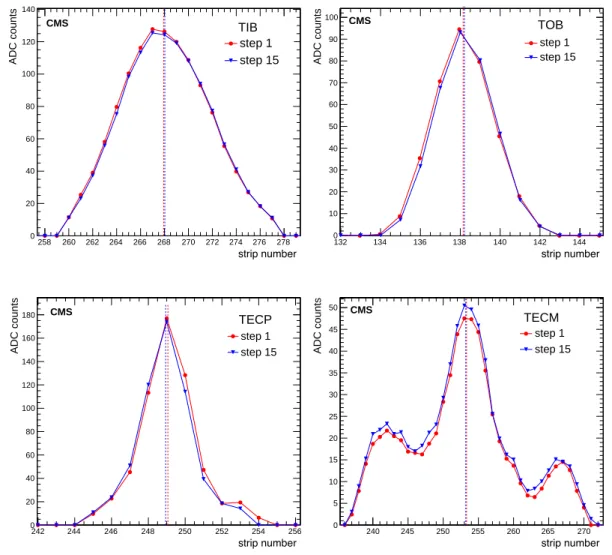
together with other alignment parameters in one global fit. Note that the laser beams passing through the mirrors or through the silicon sensors may have some kinks, but these kinks are independent of the beam orientation. The assumption of the straightness of the laser beams implies that all of the optical components of the LAS have flat surfaces near the laser beam spot, such that small displacements of the LAS components do not affect the alignment parameters. Under the above assumptions the LAS alignment procedure has two main steps: reconstruction of laser beam profiles and evaluation of alignment parameters. The laser profile is defined as an accumulated amplitude in ADC counts versus strip number within a module after 200 laser shots. The profile depends on the laser intensity, the silicon strip pitch and the width of the laser beam spot after propagation of laser light through beam splitters and mirrors. Figure 5 shows beam profiles for different subdetectors obtained in two acquisition steps. For the TOB and TIB the profiles are Gaussian-like, while for the TEC detectors, where the light passes through the silicon, the profiles show a diffraction pattern caused by reflections inside the silicon sensor. The position of the laser beam spot is obtained from the intersection of the linear extrapolations of the profile at its half-maximum.
The second step is the reconstruction of the alignment parameters with respect to the reference
position in each illuminated module. The displacements of the beam position ψj in detector
module j with respect to the reference position ψrefj are given by δj = ψj−ψrefj . These
displace-ments δjare inputs to the χ2=Σ(δj−φj(~p))2/σ2
j, where φ(~p)are the predicted displacements
depending on the fit parameters~p: αi, βi, ∆x, ∆y, Rx, Ry, Rz. For the χ2 minimization, the
∂χ2/∂pk derivatives are linearized using the small-angle approximation. The system of linear
10 4 Tracker alignment strip number 258 260 262 264 266 268 270 272 274 276 278 ADC counts 0 20 40 60 80 100 120 140 step 1 step 15 CMS TIB strip number 132 134 136 138 140 142 144 ADC counts 0 10 20 30 40 50 60 70 80 90 100 step 1 step 15 CMS TOB strip number 242 244 246 248 250 252 254 256 ADC counts 0 20 40 60 80 100 120 140 160 180 step 1 step 15 CMS TECP strip number 240 245 250 255 260 265 270 ADC counts 0 5 10 15 20 25 30 35 40 45 50 step 1 step 15 CMS TECM
Figure 5: Examples of laser beam profiles (accumulated amplitude in ADC counts for 200 laser shots vs. strip number) in the TIB, TOB, TECP, and TECM modules, obtained in two different acquisition steps. The vertical dashed line shows the reconstructed laser spot position. In the TECM, two lower diffractive peaks are visible as mentioned in the text.
LAS alignment procedure is flexible; some measurements or all measurements from a specific laser beam can be excluded from the fit, and the number of fit parameters can be varied, for example excluding rotations or offsets. These features were used to check the stability of the alignment procedure and systematic uncertainties. The results from different fit configurations agree within 10 µm.
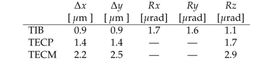
The stability of the alignment parameters reconstructed with the LAS has been studied during periods of operation at a fixed temperature where we expect no real movements of the tracker components. The stability is defined as one standard deviation of the distribution of each align-ment parameter. A summary of the LAS alignalign-ment parameters and their stability is presented
in Table 1. The best stability of about 1 µm is obtained for the relative∆x and ∆y displacements
of the TIB. For the TECM profiles the stability worsens to 2–3 µm due to larger distortion of the laser beam after passing through many mirrors.
4.2 Alignment with particle tracks 11
Table 1: Stability of alignment parameters using LAS measurements obtained during periods of operation at a fixed temperature.
∆x ∆y Rx Ry Rz
[ µm ] [ µm ] [µrad] [µrad] [µrad]
TIB 0.9 0.9 1.7 1.6 1.1
TECP 1.4 1.4 — — 1.7
TECM 2.2 2.5 — — 2.9
4.2 Alignment with particle tracks
A detailed description of tracker alignment with tracks can be found in numerous publications, e.g. in Ref. [6] and references therein. One of the track-based alignment algorithms used in
CMS is MILLEPEDE II [8]. The algorithm simultaneously reconstructs the track parameters~x
for each event and the alignment parameters~p for each alignable object, and involves two steps.
In the first step the ∂ f /∂xiand ∂ f /∂pkderivatives of the track model f(~x,~p)with respect to the
track and alignment parameters are calculated. These derivatives are stored in a matrix with
the size of(ntracksntrackpar+nalgnpar)2, where ntracksis the number of selected tracks, ntrackpar is
the number of individual track parameters (four for propagation without magnetic field and
five for propagation in the field), nalgnpar is the number of alignment parameters. Then the
corresponding system of linear equations is reduced in size using block matrix algebra and solved numerically [6].
The phase-space of particle tracks defines the sensitivity of the track-based alignment proce-dure to a particular alignment parameter. Two types of tracks can be used; tracks from col-lisions that originate in the detector centre, and tracks from cosmic rays that can cross the
detector away from the interaction point. For the 2012 period, about 15×106 collision tracks
and 4×10⁶ cosmic ray tracks were used for the alignment. The track samples are split into
separate periods in time that are used to calculate the alignment parameters for all detector modules. The intervals should be chosen such that, within each period, the operations do not
vary significantly, but at the same time should provide sufficient statistics for the MILLEPEDE
procedure. Usually, each interval corresponds to a few months of stable operation. The recon-struction accuracy of different alignment parameters in the track-based alignment depends on the number of selected tracks and on the location of the detector modules [6].
5
Tracker mechanical stability
The tracker mechanical structures have a hierarchy, and can be grouped as follows: subdetec-tors (TIB, TOB, TECs), substructures (shells, rods, petals), and individual detector modules. All these components can potentially move for different reasons and over different time scales. We distinguish between short-term variations, which occur over an interval of a few hours, and long-term variations, which occur over a period of a few days or months.
Temperature variation is expected to be the main source of movement in the tracker during physics operation. The thermal expansion of the CF composite used in the support structures
is about 2.6×10⁻⁶/◦C. For the 2.4 m long TOB this would result in displacements of about
60 µm for∆T=10◦C. Since the mechanical design of the tracker allows for thermal expansion,
the temperature-related movements should be elastic, that is, the positions are restored when the temperature is restored to its original value. However, this process can be disrupted by the uncontrollable static friction in kinematic joints and the thermal expansion of power cables, cooling pipes, etc. that are integrated into the structures of the tracker. Many thermal cycles of
12 5 Tracker mechanical stability
the tracker can thus result in some nonelastic displacements and non-rigid body deformations. The release of intrinsic stresses produced during assembly is another source of movement that can happen occasionally or be initiated by the temperature variations. Variations of the mag-netic field, intervention in the CMS cavern and mechanical work during technical stops can also cause the movement of some CMS components and affect the tracker alignment. These movements, as well as nonelastic movements and deformations, are difficult to simulate in finite-element method models, thus making experimental measurements indispensable for val-idation of the mechanical design.
5.1 Long-term stability
The long-term stability of global alignment parameters reconstructed with the LAS data in the years 2011–2013 is shown in Figure 6 and in more detail in Figures 7–10. The alignment parameters of the TIB and TECs are calculated with respect to the TOB. Each point in the plots corresponds to one LAS acquisition step with an interval of 5 minutes, and the uncertainties are from the LAS global fit. Different parameters can overlap in Figure 6, but the range of variations during the whole period is clearly visible. The operating temperature of the cooling
plants was set to +4◦C throughout the operation period, resulting in a temperature of about
+6◦C in the return pipe, which is shown as the black line in the figures. The positive spikes in
the temperature correspond to the occasional power down of the cooling plants, and the small
negative spikes of about 2◦C are due to switching off the low-voltage supplies to the detector
modules. The stability of the internal TEC alignment parameters is similar and is not discussed in this paper.
The whole period of 2011–2013 can be split into different parts. Periods with no LAS data are due to either nonoperational global CMS DAQ or nonoperational tracker. Loss of data resulting from LAS problems was below 1% and related to the occasional powering down of the LAS electronics in the service area.
Most of the LAS data were collected during periods of operation at stable temperature inside the tracker volume. The alignment parameters of the TIB and TEC are remarkably stable; all
variations in displacements are within±10 µm for the TIB,±20 µm for the TECP, and±30 µm
for the TECM. The rotations are similar. The expanded view of some typical parts shown in Figure 6 can be seen in Figure 7, for example the periods of operation at stable temperature for the TIB and TECM are presented in the upper plots.
Stable operation is often interrupted by transient periods when alignment parameters change by more than 10 µm (or 10 µrad) for TIB and 30 µm (30 µrad) for TECs during an interval of a few hours. All these periods are associated with temperature variations. The temperature can change rapidly due to occasional trips of cooling plants or, more often, due to a power trip af-fecting some detector modules. The powering down of the low voltages of the readout hybrids
reduces the temperature locally by about 15◦C. The actual temperature variations depend upon
how fast the cooling or voltages are restored, while the observed variations of the alignment parameters depend on when the LAS acquisition was restarted. The bottom left plot in Figure 7 shows an example of the evolution of the TIB alignment parameters after a power trip, affect-ing the whole tracker. Power to the tracker was restored and the LAS data acquisition restarted after 30 minutes, thus the movement during these 30 minutes was not recorded. The observed evolution of the alignment parameters follows the temperature stabilization in the tracker vol-ume, which takes about an hour. Similar effects can be observed during the powerdown of the cooling plants; in this case the expected temperature variations and, therefore, the observed displacements are bigger, as can be seen in the bottom-right plot in Figure 7. The periods with
5.1 Long-term stability 13
Figure 6: Stability of TIB, TECP, and TECM alignment parameters during 2011–2013 data tak-ing. The black line is the temperature of the cooling liquid in the return circuit.
large transient variations of alignment parameters are excluded from physics analysis.
The long periods of data taking are separated by a few technical stops when the whole CMS detector is powered down. During this time the temperature in the tracker is not controlled and is close to the ambient temperature in the detector cavern. At the same time some mechanical work and intervention to the CMS detector can take place. Hence, after each of these technical stops a new reference position is used in the LAS alignment procedure described above. The long-term evolution of the alignment parameters calculated with the LAS data is compared
14 5 Tracker mechanical stability Date 22/08/12 29/08/12 05/09/12 C o rad], Temp µ m], Rx,y,z[ µ x,y[ ∆ 25 − 20 − 15 − 10 − 5 − 0 5 10 15 20 25 ∆x y ∆ Rx Ry Rz Temp CMS TIB Date 06/05/12 13/05/12 20/05/12 27/05/12 03/06/12 10/06/12 17/06/12 C o rad], Temp µ m], Rx,y,z[ µ x,y[ ∆ 30 − 20 − 10 − 0 10 20 30 x ∆ y ∆ Rz Temp CMS TECM Date/Time 27/03/11 01:00 27/03/11 14:00 28/03/11 02:00 C o rad], Temp µ m], Rx,y,z[ µ x,y[ ∆ 25 − 20 − 15 − 10 − 5 − 0 5 10 15 20 25 x ∆ y ∆ Rx Ry Rz Temp Tracker OFF Tracker ON LAS restarted CMS TIB Date/Time 06/09/12 14:00 07/09/12 02:00 07/09/12 14:00 C o rad], Temp µ m], Rx,y,z[ µ x,y[ ∆ 25 − 20 − 15 − 10 − 5 − 0 5 10 15 20 25 x ∆ y ∆ Rx Ry Rz Temp Tracker OFF Tracker ON LAS restarted CMS TIB
Figure 7: Expanded view of the tracker alignment stability for selected time intervals. Upper left: TIB parameters during weeks of operation at stable temperature. Upper right: Variations of TECM parameters at stable temperature. Bottom left: Variations of TIB parameters after a power trip. Bottom right: TIB parameters after cooling plant shutdown and recovery.
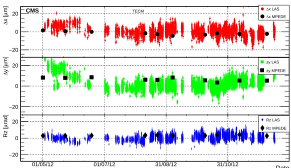
with the results obtained from the alignment with particle tracks in Figures 8–10. The align-ment parameters for the 2012 period are calculated for ten intervals that correspond to the LAS
periods with new reference positions. TheMILLEPEDEalignment configuration was similar to
the configuration for the LAS measurements, that is, the TOB position was fixed, and the TIB and TEC subdetectors were considered as rigid bodies that can move with the same degrees of
freedom as used in the LAS. SinceMILLEPEDE delivers absolute alignment parameters based
on measurements in many detector modules, whilst the LAS measures relative displacements and only for the illuminated modules, some differences between the parameters derived with the two different methods are expected. However the variations of the parameters in both mea-surements are similar and are within 30 µm (or 30 µrad), confirming the long-term mechanical stability of large structures of the tracker. The displacements below 30 µm can have different origins; for example they could be related to deformations of other components of the CMS de-tector. Since all observed large transient variations in the alignment parameters coincide with the variations of the temperature in the tracker volume, a dedicated thermal model can be used in the future to predict displacements using solely the temperature measurements.
5.2 Stability during temperature variations
Large variations of alignment parameters correlated with the temperature were studied dur-ing the long shutdown of the LHC in 2013. The tracker alignment parameters were
5.2 Stability during temperature variations 15 Date 01/05/12 01/07/12 31/08/12 31/10/12 rad] µ Rz [ 10 − 0 10 Rz LAS Rz MPEDE rad] µ Ry [ 10 − 0 10 Ry LAS Ry MPEDE rad] µ Rx [ 10 − 0 10 Rx LAS Rx MPEDE m] µ y [ ∆ 10 − 0 10 y LAS ∆ y MPEDE ∆ m] µ x [ ∆ 10 − 0 10 x LAS ∆ x MPEDE ∆ CMS TIB
Figure 8: Comparison of the TIB alignment parameters reconstructed with LAS data and
cal-culated withMILLEPEDEfrom measured particle tracks.
Date 01/05/12 01/07/12 31/08/12 31/10/12 rad] µ Rz [ 20 − 0 20 Rz LAS Rz MPEDE m] µ y [ ∆ 20 − 0 20 ∆y LAS y MPEDE ∆ m] µ x [ ∆ 20 − 0 20 ∆x LAS x MPEDE ∆ CMS TECP
Figure 9: Comparison of TECP alignment parameters measured with LAS and calculated with
MILLEPEDEfrom measured particle tracks.
then warmed up again. The evaluation of the TIB alignment parameters during temperature
transitions from+4 to −10◦C in steps of∆T = 5◦C is shown in Figure 11. The periods
with-out data are due to other CMS commissioning activities that prevented LAS operation. For all cooldown transitions the pattern of movements is rather similar; the parameters change
16 5 Tracker mechanical stability Date 01/05/12 01/07/12 31/08/12 31/10/12 rad] µ Rz [ 20 − 0 20 Rz LAS Rz MPEDE m] µ y [ ∆ 20 − 0 20 ∆y LAS y MPEDE ∆ m] µ x [ ∆ 20 − 0 20 x LAS ∆ x MPEDE ∆ CMS TECM
Figure 10: Comparison of TECM alignment parameters measured with LAS and calculated withMILLEPEDEfrom measured particle tracks.
Date/Time 02/11 13:00 06/11 01:00 C o rad], Temp µ m], Rx,y,z[ µ x,y[ ∆ 40 − 30 − 20 − 10 − 0 10 20 30 40 LAS x ∆ y ∆ Rx Ry Rz Temp MILLEPEDE x ∆ y ∆ Rx Ry Rz CMS C o +4 C o 0 0oC C o -5 C o +4 C o -10 TIB
Figure 11: Evolution of the TIB alignment parameters calculated with LAS during tracker
thermo-cycling +4 → 0 → −5 → −10 → +4◦C. The MILLEPEDE points from cosmic ray
muons are shown as open markers for the 0→ −10◦C transition.
decreases by 10 µm, and the detector rotates around the y-coordinate by about 20 µrad. Some
relaxation of the Ry rotation is observed for the long period at 0◦C. Warming up eliminates
most of the variations immediately, with some remaining residuals of about 20 µm that were not followed up in this test due to other CMS activities.
17
muons, as shown in Figure 11. About 1.6×10³and 4×10³cosmic ray tracks were recorded for
the 0◦C and−10◦C cooling steps, respectively. The MILLEPEDE configuration was similar to
the long-term stability measurements described in the previous section. The reference position
was taken at 0◦C. Despite low statistics, both measurements are in reasonable agreement for
all alignment parameters except for the Ry rotation. This rotation was weakly constrained by cosmic ray tracks because during the shutdown only the central part of the muon system was used for the trigger.
6
Summary
The mechanical stability of the CMS tracker was successfully monitored during the period 2011–2013 using a dedicated laser alignment system and particle tracks from collisions and cosmic ray muons. During the operation at stable temperatures, the variations of the alignment parameters were less than 30 µm and, in addition, larger changes were found to be related to temperature variations. These temperature-related displacements of the tracker subdetectors
are of the order of 2 µm/◦C and are largely eliminated when the temperature is restored to its
original value.
The results presented in this study have been crucial for the CMS tracker operation in cold conditions. They have established that major mechanical displacements do not take place, and have shown the importance of monitoring the temperature within the detector volume. The observed behaviour of the tracker components under various conditions reported here provides guidance for future upgrades of the CMS tracking system.
Acknowledgments
We congratulate our colleagues in the CERN accelerator departments for the excellent perfor-mance of the LHC and thank the technical and administrative staffs at CERN and at other CMS institutes for their contributions to the success of the CMS effort. In addition, we grate-fully acknowledge the computing centres and personnel of the Worldwide LHC Computing Grid for delivering so effectively the computing infrastructure essential to our analyses. Fi-nally, we acknowledge the enduring support for the construction and operation of the LHC and the CMS detector provided by the following funding agencies: the Austrian Federal Min-istry of Science, Research and Economy and the Austrian Science Fund; the Belgian Fonds de la Recherche Scientifique, and Fonds voor Wetenschappelijk Onderzoek; the Brazilian Fund-ing Agencies (CNPq, CAPES, FAPERJ, and FAPESP); the Bulgarian Ministry of Education and Science; CERN; the Chinese Academy of Sciences, Ministry of Science and Technology, and Na-tional Natural Science Foundation of China; the Colombian Funding Agency (COLCIENCIAS); the Croatian Ministry of Science, Education and Sport, and the Croatian Science Foundation; the Research Promotion Foundation, Cyprus; the Secretariat for Higher Education, Science, Technology and Innovation, Ecuador; the Ministry of Education and Research, Estonian Re-search Council via IUT23-4 and IUT23-6 and European Regional Development Fund, Estonia; the Academy of Finland, Finnish Ministry of Education and Culture, and Helsinki Institute of Physics; the Institut National de Physique Nucl´eaire et de Physique des Particules / CNRS, and Commissariat `a l’ ´Energie Atomique et aux ´Energies Alternatives / CEA, France; the Bundes-ministerium f ¨ur Bildung und Forschung, Deutsche Forschungsgemeinschaft, and Helmholtz-Gemeinschaft Deutscher Forschungszentren, Germany; the General Secretariat for Research and Technology, Greece; the National Scientific Research Foundation, and National Innova-tion Office, Hungary; the Department of Atomic Energy and the Department of Science and
18 References
Technology, India; the Institute for Studies in Theoretical Physics and Mathematics, Iran; the Science Foundation, Ireland; the Istituto Nazionale di Fisica Nucleare, Italy; the Ministry of Science, ICT and Future Planning, and National Research Foundation (NRF), Republic of Ko-rea; the Lithuanian Academy of Sciences; the Ministry of Education, and University of Malaya (Malaysia); the Mexican Funding Agencies (BUAP, CINVESTAV, CONACYT, LNS, SEP, and UASLP-FAI); the Ministry of Business, Innovation and Employment, New Zealand; the Pak-istan Atomic Energy Commission; the Ministry of Science and Higher Education and the Na-tional Science Centre, Poland; the Fundac¸˜ao para a Ciˆencia e a Tecnologia, Portugal; JINR, Dubna; the Ministry of Education and Science of the Russian Federation, the Federal Agency of Atomic Energy of the Russian Federation, Russian Academy of Sciences, the Russian Founda-tion for Basic Research and the Russian Competitiveness Program of NRNU MEPhI (M.H.U.); the Ministry of Education, Science and Technological Development of Serbia; the Secretar´ıa de Estado de Investigaci ´on, Desarrollo e Innovaci ´on and Programa Consolider-Ingenio 2010, Spain; the Swiss Funding Agencies (ETH Board, ETH Zurich, PSI, SNF, UniZH, Canton Zurich, and SER); the Ministry of Science and Technology, Taipei; the Thailand Center of Excellence in Physics, the Institute for the Promotion of Teaching Science and Technology of Thailand, Special Task Force for Activating Research and the National Science and Technology Develop-ment Agency of Thailand; the Scientific and Technical Research Council of Turkey, and Turkish Atomic Energy Authority; the National Academy of Sciences of Ukraine, and State Fund for Fundamental Researches, Ukraine; the Science and Technology Facilities Council, UK; the US Department of Energy, and the US National Science Foundation.
Individuals have received support from the Marie-Curie programme and the European Re-search Council and EPLANET (European Union); the Leventis Foundation; the A. P. Sloan Foundation; the Alexander von Humboldt Foundation; the Belgian Federal Science Policy Of-fice; the Fonds pour la Formation `a la Recherche dans l’Industrie et dans l’Agriculture (FRIA-Belgium); the Agentschap voor Innovatie door Wetenschap en Technologie (IWT-(FRIA-Belgium); the Ministry of Education, Youth and Sports (MEYS) of the Czech Republic; the Council of Sci-ence and Industrial Research, India; the HOMING PLUS programme of the Foundation for Polish Science, cofinanced from European Union, Regional Development Fund, the Mobil-ity Plus programme of the Ministry of Science and Higher Education, the National Science Center (Poland), contracts Harmonia 2014/14/M/ST2/00428, Opus 2014/13/B/ST2/02543, 2014/15/B/ST2/03998, and 2015/19/B/ST2/02861, Sonata-bis 2012/07/E/ST2/01406; the Thalis and Aristeia programmes cofinanced by EU-ESF and the Greek NSRF; the National Priorities Research Program by Qatar National Research Fund; the Programa Clar´ın-COFUND del Princi-pado de Asturias; the Rachadapisek Sompot Fund for Postdoctoral Fellowship, Chulalongkorn University and the Chulalongkorn Academic into Its 2nd Century Project Advancement Project (Thailand); and the Welch Foundation, contract C-1845.
References
[1] CMS Collaboration, “Description and performance of track and primary-vertex reconstruction with the CMS tracker”, JINST 10 (2014) P10009,
doi:10.1088/1748-0221/9/10/P10009, arXiv:1405.6569.
[2] CMS Collaboration, “The CMS experiment at the CERN LHC”, JINST 3 (2008) S08004, doi:10.1088/1748-0221/3/08/S08004.
[3] CMS Collaboration, “The CMS tracker: addendum to the Technical Design Report”, CMS Technical Design Report CERN-LHCC-2000-016, 2000.
References 19
[4] CMS Collaboration, “Alignment of the CMS silicon tracker during commissioning with cosmic rays”, JINST 5 (2010) T03009, doi:10.1088/1748-0221/5/03/T03009, arXiv:0910.2505.
[5] CMS Tracker Collaboration, “Alignment of the CMS silicon strip tracker during stand-alone commissioning”, JINST 4 (2009) T07001,
doi:10.1088/1748-0221/4/07/T07001, arXiv:0904.1220.
[6] CMS Collaboration, “Alignment of the CMS Tracker with LHC and cosmic ray data”, JINST 9 (2014) P06009, doi:10.1088/1748-0221/9/06/P06009,
arXiv:1403.2286.
[7] V. Blobel, C. Kleinwort, and F. Meier, “Fast alignment of a complex tracking detector using advanced track models”, Comp. Phys. Com. 182 (2011) 1760,
doi:10.1016/j.cpc.2011.03.017, arXiv:1103.3909.
[8] V. Blobel, “Software alignment for tracking detectors”, Nucl. Instrum. Meth. A 566 (2006) 5, doi:10.1016/j.nima.2006.05.157.
[9] B. Wittmer et al., “The laser alignment system for the CMS silicon microstrip tracker”, Nucl. Instrum. Meth. A 581 (2007) 351, doi:10.1016/j.nima.2007.08.002. [10] ALEPH Collaboration, “Monitoring the stability of the ALEPH vertex detector”, Nucl.
Phys. Proc. Suppl. 78 (1999) 301, doi:10.1016/S0920-5632(99)00561-7,
arXiv:physics/9903031.
[11] ZEUS Collaboration, “The optical alignment system of the ZEUS microvertex detector”, Nucl. Instrum. Meth. A 572 (2006) 325, doi:10.1016/j.nima.2007.06.046,
arXiv:0808.0836.
[12] AMS-02 Collaboration, “The AMS-02 tracker alignment system for 3D position control with artificial laser generated straight tracks”, Nucl. Instrum. Meth. A 572 (2006) 325,
doi:10.1016/j.nima.2006.10.273.
[13] CMS Collaboration, “Aligning the CMS muon chambers with the muon alignment system during an extended cosmic ray run”, JINST 5 (2010) T03019,
doi:10.1088/1748-0221/5/03/T03019, arXiv:0911.4770.
[14] CDF Collaboration, “The RASNIK real-time relative alignment monitor for CDF inner tracking detectors”, Nucl. Instrum. Meth. A 506 (2003) 92,
doi:10.1016/S0168-9002(03)01365-2, arXiv:hep-ex/0212025.
[15] ATLAS Collaboration, “The Optical Alignment System of the ATLAS Muon Spectrometer Endcaps”, JINST 3 (2008) P11005, doi:10.1088/1748-0221/3/11/P11005.
21
A
The CMS Collaboration
Yerevan Physics Institute, Yerevan, Armenia
A.M. Sirunyan, A. Tumasyan
Institut f ¨ur Hochenergiephysik, Wien, Austria
W. Adam, E. Asilar, T. Bergauer, J. Brandstetter, E. Brondolin, M. Dragicevic, J. Er ¨o, M. Flechl,
M. Friedl, R. Fr ¨uhwirth1, V.M. Ghete, C. Hartl, N. H ¨ormann, J. Hrubec, M. Jeitler1, A. K ¨onig,
I. Kr¨atschmer, D. Liko, T. Matsushita, I. Mikulec, D. Rabady, N. Rad, B. Rahbaran, H. Rohringer,
J. Schieck1, J. Strauss, W. Waltenberger, C.-E. Wulz1
Institute for Nuclear Problems, Minsk, Belarus
O. Dvornikov, V. Makarenko, V. Mossolov, J. Suarez Gonzalez, V. Zykunov
National Centre for Particle and High Energy Physics, Minsk, Belarus
N. Shumeiko
Universiteit Antwerpen, Antwerpen, Belgium
S. Alderweireldt, E.A. De Wolf, X. Janssen, J. Lauwers, M. Van De Klundert, H. Van Haevermaet, P. Van Mechelen, N. Van Remortel, A. Van Spilbeeck
Vrije Universiteit Brussel, Brussel, Belgium
S. Abu Zeid, F. Blekman, J. D’Hondt, N. Daci, I. De Bruyn, K. Deroover, S. Lowette, S. Moortgat, L. Moreels, A. Olbrechts, Q. Python, K. Skovpen, S. Tavernier, W. Van Doninck, P. Van Mulders, I. Van Parijs
Universit´e Libre de Bruxelles, Bruxelles, Belgium
H. Brun, B. Clerbaux, G. De Lentdecker, H. Delannoy, G. Fasanella, L. Favart, R. Goldouzian, A. Grebenyuk, G. Karapostoli, T. Lenzi, A. L´eonard, J. Luetic, T. Maerschalk, A. Marinov, A. Randle-conde, T. Seva, C. Vander Velde, P. Vanlaer, D. Vannerom, R. Yonamine, F. Zenoni,
F. Zhang2
Ghent University, Ghent, Belgium
A. Cimmino, T. Cornelis, D. Dobur, A. Fagot, M. Gul, I. Khvastunov, D. Poyraz, S. Salva, R. Sch ¨ofbeck, M. Tytgat, W. Van Driessche, E. Yazgan, N. Zaganidis
Universit´e Catholique de Louvain, Louvain-la-Neuve, Belgium
H. Bakhshiansohi, C. Beluffi3, O. Bondu, S. Brochet, G. Bruno, A. Caudron, S. De Visscher,
C. Delaere, M. Delcourt, B. Francois, A. Giammanco, A. Jafari, M. Komm, G. Krintiras, V. Lemaitre, A. Magitteri, A. Mertens, M. Musich, K. Piotrzkowski, L. Quertenmont, M. Selvaggi, M. Vidal Marono, S. Wertz
Universit´e de Mons, Mons, Belgium
N. Beliy
Centro Brasileiro de Pesquisas Fisicas, Rio de Janeiro, Brazil
W.L. Ald´a J ´unior, F.L. Alves, G.A. Alves, L. Brito, C. Hensel, A. Moraes, M.E. Pol, P. Rebello Teles
Universidade do Estado do Rio de Janeiro, Rio de Janeiro, Brazil
E. Belchior Batista Das Chagas, W. Carvalho, J. Chinellato4, A. Cust ´odio, E.M. Da Costa,
G.G. Da Silveira5, D. De Jesus Damiao, C. De Oliveira Martins, S. Fonseca De Souza,
L.M. Huertas Guativa, H. Malbouisson, D. Matos Figueiredo, C. Mora Herrera, L. Mundim,
H. Nogima, W.L. Prado Da Silva, A. Santoro, A. Sznajder, E.J. Tonelli Manganote4, F. Torres Da
22 A The CMS Collaboration
Universidade Estadual Paulistaa, Universidade Federal do ABCb, S˜ao Paulo, Brazil
S. Ahujaa, C.A. Bernardesa, S. Dograa, T.R. Fernandez Perez Tomeia, E.M. Gregoresb,
P.G. Mercadanteb, C.S. Moona, S.F. Novaesa, Sandra S. Padulaa, D. Romero Abadb, J.C. Ruiz
Vargasa
Institute for Nuclear Research and Nuclear Energy, Sofia, Bulgaria
A. Aleksandrov, R. Hadjiiska, P. Iaydjiev, M. Rodozov, S. Stoykova, G. Sultanov, M. Vutova
University of Sofia, Sofia, Bulgaria
A. Dimitrov, I. Glushkov, L. Litov, B. Pavlov, P. Petkov
Beihang University, Beijing, China
W. Fang6
Institute of High Energy Physics, Beijing, China
M. Ahmad, J.G. Bian, G.M. Chen, H.S. Chen, M. Chen, Y. Chen7, T. Cheng, C.H. Jiang,
D. Leggat, Z. Liu, F. Romeo, M. Ruan, S.M. Shaheen, A. Spiezia, J. Tao, C. Wang, Z. Wang, H. Zhang, J. Zhao
State Key Laboratory of Nuclear Physics and Technology, Peking University, Beijing, China
Y. Ban, G. Chen, Q. Li, S. Liu, Y. Mao, S.J. Qian, D. Wang, Z. Xu
Universidad de Los Andes, Bogota, Colombia
C. Avila, A. Cabrera, L.F. Chaparro Sierra, C. Florez, J.P. Gomez, C.F. Gonz´alez Hern´andez, J.D. Ruiz Alvarez, J.C. Sanabria
University of Split, Faculty of Electrical Engineering, Mechanical Engineering and Naval Architecture, Split, Croatia
N. Godinovic, D. Lelas, I. Puljak, P.M. Ribeiro Cipriano, T. Sculac
University of Split, Faculty of Science, Split, Croatia
Z. Antunovic, M. Kovac
Institute Rudjer Boskovic, Zagreb, Croatia
V. Brigljevic, D. Ferencek, K. Kadija, B. Mesic, T. Susa
University of Cyprus, Nicosia, Cyprus
A. Attikis, G. Mavromanolakis, J. Mousa, C. Nicolaou, F. Ptochos, P.A. Razis, H. Rykaczewski, D. Tsiakkouri
Charles University, Prague, Czech Republic
M. Finger8, M. Finger Jr.8
Universidad San Francisco de Quito, Quito, Ecuador
E. Carrera Jarrin
Academy of Scientific Research and Technology of the Arab Republic of Egypt, Egyptian Network of High Energy Physics, Cairo, Egypt
A. Ellithi Kamel9, M.A. Mahmoud10,11, A. Radi11,12
National Institute of Chemical Physics and Biophysics, Tallinn, Estonia
M. Kadastik, L. Perrini, M. Raidal, A. Tiko, C. Veelken
Department of Physics, University of Helsinki, Helsinki, Finland
23
Helsinki Institute of Physics, Helsinki, Finland
J. H¨ark ¨onen, T. J¨arvinen, V. Karim¨aki, R. Kinnunen, T. Lamp´en, K. Lassila-Perini, S. Lehti, T. Lind´en, P. Luukka, J. Tuominiemi, E. Tuovinen, L. Wendland
Lappeenranta University of Technology, Lappeenranta, Finland
J. Talvitie, T. Tuuva
IRFU, CEA, Universit´e Paris-Saclay, Gif-sur-Yvette, France
M. Besancon, F. Couderc, M. Dejardin, D. Denegri, B. Fabbro, J.L. Faure, C. Favaro, F. Ferri, S. Ganjour, S. Ghosh, A. Givernaud, P. Gras, G. Hamel de Monchenault, P. Jarry, I. Kucher, E. Locci, M. Machet, J. Malcles, J. Rander, A. Rosowsky, M. Titov
Laboratoire Leprince-Ringuet, Ecole Polytechnique, IN2P3-CNRS, Palaiseau, France
A. Abdulsalam, I. Antropov, S. Baffioni, F. Beaudette, P. Busson, L. Cadamuro, E. Chapon, C. Charlot, O. Davignon, R. Granier de Cassagnac, M. Jo, S. Lisniak, P. Min´e, M. Nguyen, C. Ochando, G. Ortona, P. Paganini, P. Pigard, S. Regnard, R. Salerno, Y. Sirois, T. Strebler, Y. Yilmaz, A. Zabi, A. Zghiche
Institut Pluridisciplinaire Hubert Curien (IPHC), Universit´e de Strasbourg, CNRS-IN2P3
J.-L. Agram13, J. Andrea, A. Aubin, D. Bloch, J.-M. Brom, M. Buttignol, E.C. Chabert,
N. Chanon, C. Collard, E. Conte13, X. Coubez, J.-C. Fontaine13, D. Gel´e, U. Goerlach, A.-C. Le
Bihan, P. Van Hove
Centre de Calcul de l’Institut National de Physique Nucleaire et de Physique des Particules, CNRS/IN2P3, Villeurbanne, France
S. Gadrat
Universit´e de Lyon, Universit´e Claude Bernard Lyon 1, CNRS-IN2P3, Institut de Physique Nucl´eaire de Lyon, Villeurbanne, France
S. Beauceron, C. Bernet, G. Boudoul, C.A. Carrillo Montoya, R. Chierici, D. Contardo, B. Courbon, P. Depasse, H. El Mamouni, J. Fay, S. Gascon, M. Gouzevitch, G. Grenier, B. Ille,
F. Lagarde, I.B. Laktineh, M. Lethuillier, L. Mirabito, A.L. Pequegnot, S. Perries, A. Popov14,
D. Sabes, V. Sordini, M. Vander Donckt, P. Verdier, S. Viret
Georgian Technical University, Tbilisi, Georgia
T. Toriashvili15
Tbilisi State University, Tbilisi, Georgia
D. Lomidze
RWTH Aachen University, I. Physikalisches Institut, Aachen, Germany
C. Autermann, S. Beranek, L. Feld, M.K. Kiesel, K. Klein, M. Lipinski, M. Preuten, C. Schomakers, J. Schulz, T. Verlage
RWTH Aachen University, III. Physikalisches Institut A, Aachen, Germany
A. Albert, M. Brodski, E. Dietz-Laursonn, D. Duchardt, M. Endres, M. Erdmann, S. Erdweg, T. Esch, R. Fischer, A. G ¨uth, M. Hamer, T. Hebbeker, C. Heidemann, K. Hoepfner, S. Knutzen, M. Merschmeyer, A. Meyer, P. Millet, S. Mukherjee, M. Olschewski, K. Padeken, T. Pook, M. Radziej, H. Reithler, M. Rieger, F. Scheuch, L. Sonnenschein, D. Teyssier, S. Th ¨uer
RWTH Aachen University, III. Physikalisches Institut B, Aachen, Germany
V. Cherepanov, G. Fl ¨ugge, B. Kargoll, T. Kress, A. K ¨unsken, J. Lingemann, T. M ¨uller,
24 A The CMS Collaboration
Deutsches Elektronen-Synchrotron, Hamburg, Germany
M. Aldaya Martin, T. Arndt, C. Asawatangtrakuldee, K. Beernaert, O. Behnke, U. Behrens,
A.A. Bin Anuar, K. Borras17, A. Campbell, P. Connor, C. Contreras-Campana, F. Costanza,
C. Diez Pardos, G. Dolinska, G. Eckerlin, D. Eckstein, T. Eichhorn, E. Eren, E. Gallo18,
J. Garay Garcia, A. Geiser, A. Gizhko, J.M. Grados Luyando, A. Grohsjean, P. Gunnellini,
A. Harb, J. Hauk, M. Hempel19, H. Jung, A. Kalogeropoulos, O. Karacheban19, M. Kasemann,
J. Keaveney, C. Kleinwort, I. Korol, D. Kr ¨ucker, W. Lange, A. Lelek, T. Lenz, J. Leonard,
K. Lipka, A. Lobanov, W. Lohmann19, R. Mankel, I.-A. Melzer-Pellmann, A.B. Meyer, G. Mittag,
J. Mnich, A. Mussgiller, D. Pitzl, R. Placakyte, A. Raspereza, B. Roland, M. ¨O. Sahin, P. Saxena,
T. Schoerner-Sadenius, S. Spannagel, N. Stefaniuk, G.P. Van Onsem, R. Walsh, C. Wissing
University of Hamburg, Hamburg, Germany
V. Blobel, M. Centis Vignali, A.R. Draeger, T. Dreyer, E. Garutti, D. Gonzalez, J. Haller, M. Hoffmann, A. Junkes, R. Klanner, R. Kogler, N. Kovalchuk, T. Lapsien, I. Marchesini,
D. Marconi, M. Meyer, M. Niedziela, D. Nowatschin, F. Pantaleo16, T. Peiffer, A. Perieanu,
J. Poehlsen, C. Scharf, P. Schleper, A. Schmidt, S. Schumann, J. Schwandt, H. Stadie, G. Steinbr ¨uck, F.M. Stober, M. St ¨over, H. Tholen, D. Troendle, E. Usai, L. Vanelderen, A. Vanhoefer, B. Vormwald
Institut f ¨ur Experimentelle Kernphysik, Karlsruhe, Germany
M. Akbiyik, C. Barth, S. Baur, C. Baus, J. Berger, E. Butz, R. Caspart, T. Chwalek, F. Colombo, W. De Boer, A. Dierlamm, S. Fink, B. Freund, R. Friese, M. Giffels, A. Gilbert, P. Goldenzweig,
D. Haitz, F. Hartmann16, S.M. Heindl, U. Husemann, I. Katkov14, S. Kudella, H. Mildner,
M.U. Mozer, Th. M ¨uller, M. Plagge, G. Quast, K. Rabbertz, S. R ¨ocker, F. Roscher, M. Schr ¨oder, I. Shvetsov, G. Sieber, H.J. Simonis, R. Ulrich, S. Wayand, M. Weber, T. Weiler, S. Williamson, C. W ¨ohrmann, R. Wolf
Institute of Nuclear and Particle Physics (INPP), NCSR Demokritos, Aghia Paraskevi, Greece
G. Anagnostou, G. Daskalakis, T. Geralis, V.A. Giakoumopoulou, A. Kyriakis, D. Loukas, I. Topsis-Giotis
National and Kapodistrian University of Athens, Athens, Greece
S. Kesisoglou, A. Panagiotou, N. Saoulidou, E. Tziaferi
University of Io´annina, Io´annina, Greece
I. Evangelou, G. Flouris, C. Foudas, P. Kokkas, N. Loukas, N. Manthos, I. Papadopoulos, E. Paradas
MTA-ELTE Lend ¨ulet CMS Particle and Nuclear Physics Group, E ¨otv ¨os Lor´and University, Budapest, Hungary
N. Filipovic, G. Pasztor
Wigner Research Centre for Physics, Budapest, Hungary
G. Bencze, C. Hajdu, D. Horvath20, F. Sikler, V. Veszpremi, G. Vesztergombi21, A.J. Zsigmond
Institute of Nuclear Research ATOMKI, Debrecen, Hungary
N. Beni, S. Czellar, J. Karancsi22, A. Makovec, J. Molnar, Z. Szillasi
Institute of Physics, University of Debrecen
M. Bart ´ok21, P. Raics, Z.L. Trocsanyi, B. Ujvari
Indian Institute of Science (IISc)
25
National Institute of Science Education and Research, Bhubaneswar, India
S. Bahinipati23, S. Bhowmik24, S. Choudhury25, P. Mal, K. Mandal, A. Nayak26, D.K. Sahoo23,
N. Sahoo, S.K. Swain
Panjab University, Chandigarh, India
S. Bansal, S.B. Beri, V. Bhatnagar, R. Chawla, U.Bhawandeep, A.K. Kalsi, A. Kaur, M. Kaur, R. Kumar, P. Kumari, A. Mehta, M. Mittal, J.B. Singh, G. Walia
University of Delhi, Delhi, India
Ashok Kumar, A. Bhardwaj, B.C. Choudhary, R.B. Garg, S. Keshri, S. Malhotra, M. Naimuddin, K. Ranjan, R. Sharma, V. Sharma
Saha Institute of Nuclear Physics, Kolkata, India
R. Bhattacharya, S. Bhattacharya, K. Chatterjee, S. Dey, S. Dutt, S. Dutta, S. Ghosh, N. Majumdar, A. Modak, K. Mondal, S. Mukhopadhyay, S. Nandan, A. Purohit, A. Roy, D. Roy, S. Roy Chowdhury, S. Sarkar, M. Sharan, S. Thakur
Indian Institute of Technology Madras, Madras, India
P.K. Behera
Bhabha Atomic Research Centre, Mumbai, India
R. Chudasama, D. Dutta, V. Jha, V. Kumar, A.K. Mohanty16, P.K. Netrakanti, L.M. Pant,
P. Shukla, A. Topkar
Tata Institute of Fundamental Research-A, Mumbai, India
T. Aziz, S. Dugad, G. Kole, B. Mahakud, S. Mitra, G.B. Mohanty, B. Parida, N. Sur, B. Sutar
Tata Institute of Fundamental Research-B, Mumbai, India
S. Banerjee, R.K. Dewanjee, S. Ganguly, M. Guchait, Sa. Jain, S. Kumar, M. Maity24,
G. Majumder, K. Mazumdar, T. Sarkar24, N. Wickramage27
Indian Institute of Science Education and Research (IISER), Pune, India
S. Chauhan, S. Dube, V. Hegde, A. Kapoor, K. Kothekar, S. Pandey, A. Rane, S. Sharma
Institute for Research in Fundamental Sciences (IPM), Tehran, Iran
S. Chenarani28, E. Eskandari Tadavani, S.M. Etesami28, M. Khakzad, M. Mohammadi
Najafabadi, M. Naseri, S. Paktinat Mehdiabadi29, F. Rezaei Hosseinabadi, B. Safarzadeh30,
M. Zeinali
University College Dublin, Dublin, Ireland
M. Felcini, M. Grunewald
INFN Sezione di Baria, Universit`a di Barib, Politecnico di Baric, Bari, Italy
M. Abbresciaa,b, C. Calabriaa,b, C. Caputoa,b, A. Colaleoa, D. Creanzaa,c, L. Cristellaa,b, N. De
Filippisa,c, M. De Palmaa,b, L. Fiorea, G. Iasellia,c, G. Maggia,c, M. Maggia, G. Minielloa,b,
S. Mya,b, S. Nuzzoa,b, A. Pompilia,b, G. Pugliesea,c, R. Radognaa,b, A. Ranieria, G. Selvaggia,b,
A. Sharmaa, L. Silvestrisa,16, R. Vendittia,b, P. Verwilligena
INFN Sezione di Bolognaa, Universit`a di Bolognab, Bologna, Italy
G. Abbiendia, C. Battilana, D. Bonacorsia,b, S. Braibant-Giacomellia,b, L. Brigliadoria,b,
R. Campaninia,b, P. Capiluppia,b, A. Castroa,b, F.R. Cavalloa, S.S. Chhibraa,b, G. Codispotia,b,
M. Cuffiania,b, G.M. Dallavallea, F. Fabbria, A. Fanfania,b, D. Fasanellaa,b, P. Giacomellia,
C. Grandia, L. Guiduccia,b, S. Marcellinia, G. Masettia, A. Montanaria, F.L. Navarriaa,b,