F tests with random samples size.
Theory and applications
Elsa E. Moreiraa,∗, Jo˜ao T. Mexiaa, Christoph E. Minderb
a
CMA - Center of Mathematics and Applications, Faculty of Sciences and Technology, Nova University of Lisbon, Campus Caparica, 2829-516 Caparica, Portugal
b
Horten Zentum, Medical Faculty, University of Zurich
Abstract
Given a time span for collecting observations in a comparison study, it is advisable to consider the samples size of the ANOVA levels as random vari-ables. More powerful F tests with F distribution conditional to N = n, leading to lower critical values, are developed. The approach is used to ob-tain the minimum duration for the data collection that ensures a pre-fixed test power.
Keywords: ANOVA, F distribution, Pathologies comparison, Poisson distribution, Power analysis
1. Introduction
The theoretical developments presented in this paper were motivated by a real case situation in the field of medicine. Consider the numbers of patients that arrive to an hospital with different pathologies during a given time span. These numbers cannot be known in advance because, if we decide to do the counting in a different time period of the same length, the number of patients obtained with those pathologies will be different from the first counting. So, if, due to limitations in the budget, we have to conduct just one study to compare the pathologies, it is more correct to consider the sample dimensions as realizations of random variables. The data will be collected from the patients with each pathology as soon as they present themselves.
∗Corresponding author
This situation arises mostly because there is a given time span for collect-ing the observations. After the elapsed time interval, the F test statistics can be obtained to test hypotheses about the different means values. In what fol-lows, it is assumed that the sample dimensions n1, ..., nkfor the k pathologies
are realizations of independent Poisson variables with parameters λ1, ..., λk
and the observations in these sample are normal, independent with variance σ2. As a result, the F statistic to test the null hypotheses H
0 : µ1 = ... = µk
will have conditional F distribution on the number of observations as will be seen in the next section.
The approach presented is also useful while planning studies, before the data are in. The minimum data collection duration to ensure, with a given probability, reliable results will be obtained. Thus, when all k pathologies are covered, the conditional distribution of the F test statistic has k − 1 and n − k degrees of freedom, with n the sum of all ni, i = 1, ..., k and
non-centrality parameter δ, which is null when the mean values µ1, ..., µk
for different pathologies are equal. Thus, δ will measure the “distance” of the alternatives from H0. So, we may look for the minimum duration that
ensures, with a given probability, that all pathologies have at least a minimum number of observations that allow the conditional power of the α level test for a given δ to be sufficient high. Therefore, in sub-section 3.1, we see how to determine these minimum samples sizes ˙ni, i = 1, ..., k to have a sufficient
powerful F test, while in sub-section 3.2, the minimum time span for, with a probability p, getting these ˙n1, ..., ˙nk is obtained. Finally, an application
with simulated data is presented in section 5 to illustrate the methodology. 2. Conditional F distributions
Let the components of the vector n = (n1, ..., nk) of the samples sizes
be realizations of the components of the vector N = (N1, ..., Nk). The
com-ponents of N are independent Poisson variables, with vector of parameters λ = (λ1, ..., λk). Assuming that, when n > 0, the samples xi,1, ..., xi,n
i,
i = 1, ..., k are normal with mean values µ1, ..., µk and variance σ2, for
test-ing H0 : µ1 = ... = µk the F test statistic
F = n − k k − 1 Pk i=1 T2 i ni − T2 n Pk i=1Si is used, where Ti = Pn i j=1xi,j, Si = Pni
j=1x2i,j − Ti2/ni, T = Pki=1Ti and
Due to our assumption for N, the F statistics will have F distribution conditional to N = n, with k − 1 and n − k degrees of freedom and non-centrality parameter δ = 1 σ2 k X i=1 ni(µi− µ.)2 where µ. = 1 n k X i=1 niµi
is the general mean value (Hocking, 2003; Mexia, 1990).
In a previous paper (Mexia and Moreira, 2010) the unconditional distri-bution for the F statistics was derived. This distridistri-bution is given by the following series
˙
F (z) =X
n>0
q(n)F (z|k − 1, n − k, δ(n)) (1)
whose terms corresponds to all the vectors n = (n1, ..., nk) with ni > 0, i =
1, ..., k and where q(n) = k Y i=1 e−λiλini ni! 1 − e−λi.
However, when the null hypothesis H0 : µ1 = ... = µkholds, δ(n) = 0, ∀n > 0
and
F ∼ ˙F0(z) =
X
n>0
q(n)F (z|k − 1, n − k). (2)
Notice that in eq. (1), the n for the degrees of freedom of the denominator does not change within the sum.
To compute the values of ˙F0(z) the corresponding series in eq. (2) must
be obviously truncated. The truncation error of this series when restricting ourselves to samples with n ≤ no was studied in a previous paper (Mexia
and Moreira, 2010). In that paper, it was shown that the truncation error does not exceed a bound
b(no) < kε
(1 − e−λo)k,
if each no
i, the components of no, are chosen such no i X ni=0 e−λiλ ni i ni! > 1 − ε, i = 1, ..., k, (3)
with ε small (Mexia and Moreira, 2010). So, from this inequality we can obtain the minimal samples sizes that allow us to control the truncation error for the distribution ˙F0(z).
In Table 1 is presented for different values of the minimal average sample size, λo = Min{λ
1, ..., λk} and different small ε, the minimal samples
dimen-sion no to have satisfy inequality (3). These truncation errors are perfectly
controlled even if the samples dimensions are relatively small, i.e., for in-stance for k = 3, if the minimum of the λi, i = 1, 2, 3 is λ0 = 1, for ε = 10−6
the sample dimensions should not be less than 9. In this example, the trun-Table 1: The minimal dimension of the samples no required to have the truncation error controlled λo 1 2 5 10 20 ε= 10−4 6 9 15 24 39 ε= 10−6 9 12 19 28 45 ε= 10−8 11 14 22 32 50
cation error has an upper bound of 0.000012. The critical values tables in common use have in general 3 decimal places of precision, thus truncating the distribution with an error of 0.000012 is more than needed to get a critical value with good accuracy.
Theses formulas enable us to solve the equation ˙F0(z) = 1 − α for z,
to obtain the (1 − α)-th quantiles, i.e, the critical values of α level tests. After obtaining the quantiles for the distribution ˙F0(z), the inference for the
one-way ANOVA to compare the k pathologies proceeds in the usual way (Scheff´e, 1959; Montgomery, 1997).
In order to demonstrate the advantage of using F tests with random samples size, abbreviated ˙F tests, we were led to obtain several critical values for 5% of probability for the case of a test with 3 pathologies and compare these with the critical values using an usual F test. The values, presented in Table 3, were computed assuming increasing different values for λ1, λ2 and
λ3 that originate consequently different values of n. In Figure 1 the curves
for the critical values in Table 2 are presented. From that Figure we see that the critical values for the ˙F test are always lower than the critical values for the usual F test. Although, the difference between both decrease and tend to 0 as n increases.
Table 2: Critical values for F tests with random sample size and for usual F tests, case for compare 3 pathologies
Critical Values (5%) λ1 λ2 λ3 n F˙ F 0,05 0,05 0,05 9 4.256 5.143 0,1 0,1 0,1 12 3.885 4.256 0,1 0,3 0,5 16 3.634 3.806 1 1 1 27 3.354 3.403 2 2 1 33 3.285 3.316 4 3 2 43 3.214 3.232 5 4 4 53 3.172 3.183 6 5 4 57 3.159 3.168 8 8 6 71 3.126 3.132 11 11 10 88 3.100 3.104 16 16 16 114 3.076 3.078 3. Power analysis
Power analysis using the statistical power of a hypothesis test also called sample size analysis, is an important tool for deciding what sample size is required to guarantee a reasonable chance to reject a false null hypothesis. In the next two sub-sections, we are going use the power analysis under the context of random samples size to obtain first, the minimum dimensions ni,
i = 1, ..., k that the samples must have and second, the minimum duration for the data collection in order to obtain that minimal dimensions.
3.1. Obtaining the global sample dimension
Suppose that we are working with F tests for fixed effect models for which, a null hypotheses H0 and an alternative one Ha were previously formulated.
Considering a study with k pathologies and that n represents the sum of sample dimensions for all pathologies, the power function of this tests is given by
P owα(δ) = P r(F > f1−α,k−1,n−k|H0 false) = 1 − β,
where f1−α,k−1,n−k is the (1−α)-th quantile of the central F distribution with k − 1 and n − k degrees of freedom. Since P r(F > f1−α,k−1,n−k|H0 false) =
1 − F (f1−α,k−1,n−k|k − 1, n − k, δ) we have
F (f1−α,k−1,n−k|k − 1, n − k, δ) = β. (4)
Since the power of the F text is a monotonically increasing function of the parameter δ, from equation (4) we can get the pairs of (n, δ) that allow
Figure 1: Critical valor for 5% probability level ˙F versus F test
obtaining a predetermined power 1 − β for the α-level F test with k − 1 and n − k degrees of freedom. From those pairs, we can choose a minimum global sample size n that guarantees, for all alternatives with non-centrality parameter not less than a given δ, a test power of at least 1−β. We point out that the parameter δ measures the “distance” between the alternatives and the tested hypothesis. Thus, in an usual F test we can look for the minimum sample size n that, for a given δ, ensures a sufficient power for the test.
However, for obtaining the power of the F test with random samples size, we should use the ˙F distribution and the ˙f1−α,k−1,n−k quantil, that is
˙
F ( ˙f1−α,k−1,n−k) =X
n>0
q(n)F ( ˙f1−α,k−1,n−k|k − 1, n − k, δ(n)). (5) For the computation of ˙F distribution, as described in section 2, we have to know the frequencies λ1, ..., λk and obtain the minimal sizes n1, ..., nk of the
samples that allow to truncate the series and compute with enough precision the distribution values. The sum of all ni give us a minimum n and then we
can obtain the quantil ˙f1−α,k−1,n−k. Moreover, in computing the non-central
˙
F , since in eq. (5) the non-centrality parameter δ(n) has to be computed in each step of the sum, we need also to fixate the values of the sample means µ1, ..., µk and variance σ2 based on previous knowledge. The power function
for this specific ˙F test is given by
If the obtained power is not enough, we should increase the n1, ..., nk
propor-tionally without changing the λ1, ..., λk and recalculate the power until we
have obtained a reasonable value. A reasonable value for the power will be for instance 80%. This procedure may be repeated with different assumptions of sample means values µ1, ..., µk and σ2, in order to obtain a final conclusion
about the minimum n that guaranties sufficient power for the test. Lets call to these minimum dimensions ˙n1, ..., ˙nk and to their sum ˙n.
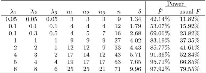
In Table 3 we present the comparative results for the power of an ˙F and F usual test with 3 pathologies (k = 3). These results were obtained assuming different values of λ1, λ2, λ3 and with µ1, µ2, µ3 and σ2 constant. Notice that
the n1, n2, n3 obtained are the minimum that allow a good precision in the ˙F
distribution values. For all the cases presented in Table 3 the power of the ˙F test is considerably higher than the power of the usual F test, this meaning that the F tests considering F distributions that account on the randomness of samples size have an higher probability of reject a false null hypothesis. Table 3: Comparison between the power of ˙F tests (F tests with random samples size) and the usual F tests; case for comparing 3 pathologies and µ1= 0.5, µ2= 0.3, µ3= 1.2, σ2 = 1. Power λ1 λ2 λ3 n1 n2 n3 n δ F˙ usual F 0.05 0.05 0.05 3 3 3 9 1.34 42.14% 11.82% 0.1 0.1 0.1 4 4 4 12 1.79 53.07% 15.92% 0.1 0.3 0.5 4 5 7 16 2.68 69.06% 23.82% 1 1 1 9 9 9 27 4.02 83.19% 37.35% 2 2 1 12 12 9 33 4.43 85.77% 41.61% 4 3 2 17 14 12 43 5.71 91.36% 52.84% 5 4 4 19 17 17 53 7.65 95.71% 66.85% 8 8 6 25 25 21 71 9.96 97.92% 79.55%
Considering now, for instance, the second example in Table 3 (λ1 =
λ2 = λ3 = 0.1), the power obtained 53.07% for the minimum n1, n2, n3 and
those µ1, µ2, µ3, σ2, is not sufficient high, thus we proportionally increase the
n1, n2, n3 without changing the λ1, λ2, λ3 until obtaining a power near 80%
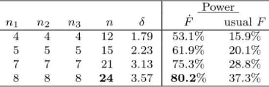
as showed in the Table 4. This power is obtained for an n = 24. If we think the sample means and variance can change significantly in order to cause a decrease of the δ, we must also calculate the power for several different values of these parameters and obtain the n that allows a power of at least 80%.
Table 4: Power of an ˙F test with λ1 = λ2 = λ3 = 0.1 and µ1 = 0.5, µ2 = 0.3, µ3 = 1.2, σ2
= 1 for increasing n1, n2, n3until obtaining 80% in comparison with the power of the the usual F Test
Power n1 n2 n3 n δ F˙ usual F 4 4 4 12 1.79 53.1% 15.9% 5 5 5 15 2.23 61.9% 20.1% 7 7 7 21 3.13 75.3% 28.8% 8 8 8 24 3.57 80.2% 37.3%
3.2. Obtaining the minimum duration by sampling
In the last section, the minimum sample dimensions ˙ni, i = 1, ..., k and
global dimension ˙n to get an ˙F test with power larger than or equal to 1 − β were obtained. Now, we may want to know how much time is necessary to wait in order to get this minimum number of observations.
Assuming the existence of k independent Poisson counting processes Ni(t);
t ≥ 0, i = 1, ..., k, corresponding to the arrivals of the patients with the k pathologies, and reliable lower bounds ˙λ1, ..., ˙λk for the processes intensities,
the probability of getting at least ˙ninumber of patients for the i-th pathology,
for all i = 1, .., k, is pr(N(t) ≥ ˙n) = k Y i=1 pr(Ni(t) ≥ ˙ni) = k Y i=1 [1 − pr(Ni(t) < ˙ni)] ≥ k Y i=1 [1 − ˙ni−1 X j=1 e− ˙λit( ˙λit) j j! ]. (7)
since for the lower bounds ˙λ1, ..., ˙λk we have
pr(Ni(t) < ˙ni) < ˙ni−1 X j=1 e− ˙λit( ˙λit) j j! , for i = 1, ..., k.
Now, setting a probability p to have N(t) ≥ ˙n, the time t can be chosen such that k Y i=1 [1 − ˙ni−1 X j=1 e− ˙λit( ˙λit) j j! ] > p. (8)
4. An example of application
In order to illustrate the usefulness of the method, in this section an example of application with non real data is presented.
Consider the people arriving at an hospital with pathologies 1, 2 and 3 during a given time span, from which a blood sample is taken to register a specific value. Suppose that is known from previous studies that the arrivals rates for the 3 pathologies are λ1 = 8.56, λ2 = 0.64 and λ3 = 0.34 cases per
day, in that hospital.
Before moving to data collection, we may want to answer to the following questions:
1. What are the minimum samples sizes required to have a controlled truncation error for the series distribution in eq. (2), therefore enough precision for the ˙F distribution?
2. Are these minimum samples sizes sufficient to obtain a pre-fixed test power of 80%? Do we need more observations in order to get that? 3. How long is required to wait to obtain these minimum samples sizes? In the next section the answers to those questions will be given. After that, we can proceed with the analysis of the collected data.
4.1. Planning the study
In order to answer to question 1, we use the inequality (3) to computed the minimum samples sizes for the 3 pathologies. The results are presented in Table 5 taking ε = 10−6. If these minimum samples size are satisfied, we are
Table 5: Minimum samples sizes
pathology 1 2 3
λi 8.56 0.64 0.34
ni min. 26 7 6
guaranteed that the truncation error will have an upper bound of 0.0001230, which give us enough precision on the critical values.
An F test to compare k = 3 different pathologies with α = 5% of signif-icance will have an F statistic with 2 and n − 3 degrees of freedom. So, we start by obtaining the power of the corresponding ˙F test for the minimum samples sizes in Table 5 (n = 39). To this purpose, we used the known estimates for the sample means values: ˆµ1 = 0.91, ˆµ1 = 1.5, ˆµ1 = 0.7; and
variance: ˆσ2 = 0.4. The power obtained, 92.9% for a δ = 6.23, is high
enough, thus we do not need to increase the ni, i = 1, 2, 3. As a result, the
minimum global sample size of 39 corresponding to the sum of the minimum samples sizes in Table 5, enables us to conduct an ˙F test with a power much higher that 80%.
Now, let’s consider a probability p = 1 − ε of getting n1 ≥ 26 ∩ n2 ≥
7 ∩ n3 ≥ 6, with ε = 10−4. We computed the probability given by expression
(8) for t increasing from 1 to 100 and stopping when pr(n1 ≥ 0 ∩ n2 ≥
0 ∩ n3 ≥ 0) > p and found out that for t ≃ 58 the value for that probability
was 0.99991. In other words, the data collection period should be at least 58 days in order to obtain that number of observations per pathology.
4.2. Data analysis
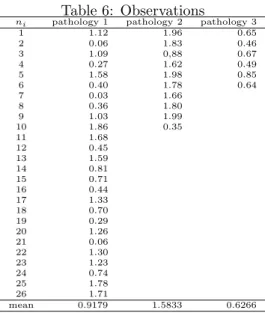
A study was conducted with a collection period of 58 days and the 42 observations presented in Table 6 were collected.
Table 6: Observations
ni pathology 1 pathology 2 pathology 3
1 1.12 1.96 0.65 2 0.06 1.83 0.46 3 1.09 0,88 0.67 4 0.27 1.62 0.49 5 1.58 1.98 0.85 6 0.40 1.78 0.64 7 0.03 1.66 8 0.36 1.80 9 1.03 1.99 10 1.86 0.35 11 1.68 12 0.45 13 1.59 14 0.81 15 0.71 16 0.44 17 1.33 18 0.70 19 0.29 20 1.26 21 0.06 22 1.30 23 1.23 24 0.74 25 1.78 26 1.71 mean 0.9179 1.5833 0.6266
In Table 7 is presented the one way ANOVA used to test the null hypoth-esis H0 : µ1 = µ2 = µ3.
The distribution ˙F0(z) =
P
n>0q(n)F (z|2, 39) of the F statistic was
com-puted and the corresponding series was truncated, that is, the terms such n1 > 26 ∧ n2 > 10 ∧ n3 > 6 were not considered. This condition guaranties
Table 7: One way ANOVA table
ANOVA df SS F statistic δ
Treatments 2 4.365 7.515 11.2
Error 39 11.326
Total 41 15.691
Using a numerical method the equation ˙F0(z) = 0.95 was solved in order
to z and obtained the quantile ˙f(0.95;2;39), which is the critical value of the 0.05
level test. Since the obtained critical value 3.220 is less than the F = 7.515, the null hypothesis is rejected and we can conclude that the 3 pathologies are significantly different. Moreover, since the obtained samples led to an higher δ = 11.2 (Table 7) and n = 42, the power for this test is 99.29% even higher then planed, in contrast with the 82.96% of the usual F test.
Had we considered the samples sizes n1, n2, n3 as fixed numbers rather
than as Poisson random variables, the critical value for this test with the usual central F distribution would be 3.238 instead of 3.220. As a result, when using F tests with random samples size, a slightly smaller value for the F statistic is required. However, the power of the test using the ˙F distribution, i.e., considering random samples size, increase considerably comparatively with the power of the usual F test.
All the computations were performed using the EXCEL and programming in Microsoft Visual Basic for applications.
5. Conclusions
In comparison studies, when there is a specific time span to collect the observations and the sizes of the samples cannot be decided previously, it is appropriate to consider the sample dimensions as realizations of independent Poisson variables. The F tests developed from this assumption have the advantage of being more powerful, i.e., F tests considering F distributions that account on the randomness of samples size have an higher probability of reject a false null hypothesis. Moreover, they generate smaller critical values than the F usual distribution, the difference tending to zero as the number of observations increase. Furthermore, the approach is useful in the planning phase of a study to obtain the minimum duration for the data collection that ensures the chosen power and level of significance.
Acknowledgements
This work was partially supported by CMA/FCT/UNL, under the project PEst-OE/MAT/UI0297/2011.
References
Hocking, R., 2003. Methods and Applications of Linear Models. John Wil-ley&Sons. New York.
Kendall, M. and Stuart, A., 1961. The Advanced Theory of Statistics. Vol.II. Charles Griffin & Co. Londres.
Montgomery, D.C., 1997. Design and Analysis of Experiments - 5th edition. John Willey & Sons. New York.
Mexia, J.T., Nunes, C., Ferreira, D., Ferreira, S., Moreira, E., 2011. Ortog-onal fixed efects ANOVA with random sample sizes. WSEAS proceedings of the 5th International conference on Applied Mathematics, Simulation, Modelling, 84-90.
Mexia, J.T., Moreira, E.E., 2010. Randomized sample size F tests for the one-way layout. AIP Conference Proceedings, volume 1281- ICNAAM 2010-8th International Conference of Numerical Analysis and Applied Mathe-matics, 1248-1251,doi:10.1063/1.3497917.
Mexia, J.T., 1990. Best linear unbiased estimates, duality of F tests and Sheff multiple comparison method in presence of controlled heteroscedasticity. Computational statistics and data analisys 10(3), 271-281.
Nunes, C., Ferreira, D., Ferreira, S., Mexia, J.T., 2011. F-tests with a rare pathology. Journal of Applied Statistics. DOI:10.1080/02664763.2011.603293.