Mathematical and numerical modeling of turbulent
reactive flows using a hybrid LES / PDF methodology
UNIVERSIDADE FEDERAL DE UBERL ˆ
ANDIA
FACULDADE DE ENGENHARIA MEC ˆ
ANICA
Pour l’obtention du Grade de
DOCTEUR DE L’ECOLE NATIONALE SUPERIEURE DE
MECANIQUE ET D’AEROTECHNIQUE
( Diplˆome National - Arrˆet´e du 7 aoˆut 2006 )
Ecole Doctorale : Sciences Pour l’Ing´enieur et A´eronautique Secteur de Recherche : Energ´etique, Thermique, Combustion
Pr´esent´ee par:
Jo˜
ao Marcelo VEDOVOTO
**************************************************************
Mathematical and numerical modeling of turbulent
reactive flows using a hybrid LES / PDF methodology
************************************************************** Directeurs de Th`ese : Arnaud MURA etAristeu da SILVEIRA NETO
************************************************************** Soutenue le 18 Novembre 2011 devant la commission d’examen **************************************************************
Jury
-M. P. HALDENWANG, - Professeur Universit´e de Provence Marseille, Rapporteur M. D.A. RADE, - Professeur UFU Uberlandia, Rapporteur
M. J. REVEILLON, - Professeur Universit´e de Rouen, Examinateur M. F.J. SOUZA, - Professeur UFU Uberlandia, Examinateur
M. L.F. FIGUEIRA DA SILVA, - Professeur PUC-Rio, Rio de Janeiro, Examinateur M. A. DA SILVEIRA NETO, - Professeur UFU, Uberlandia
Mathematical and numerical modeling of turbulent
reactive flows using a hybrid LES / PDF methodology
Tese apresentada ao Programa de P´os-gradua¸c˜ao em Engenharia Mecˆanica da Universidade Federal de Uberlˆandia e a Es-cola doutoral da ´Ecole Nationale Sup´erieure de M´ecanique et d’A´erotechnique - ENSMA, como parte dos requisitos para a obten¸c˜ao do t´ıtulo de DOUTOR EM ENGENHARIA
MEC ˆANICA e DOCTEUR DE L’ENSMA.
´
Area de concentra¸c˜ao: Transferˆencia de Calor e Mecˆanica dos Fluidos.
Orientadores: Prof. Dr. Aristeu da Silveira Neto e Dr. Arnaud Mura
Co-Orientador: Prof. Dr. Luis Fernando Figueira da Silva
!" #
$ % % &
$' ()* + , $ ' + - # ./ ../ % 0
-1 0 2 * 3 2
-# 0 ( , , *
-4 5 6 , 6 7
8 #9 ) $ 7 ) :
3 * ;< < = >2< $ = %
-- ) $ 7 # 4 - .- ) # 4 - ?-@ # 4 - - * ; # 4 -* 3 2 !AA# - 2 - - * ( ,
, - - 6 , 6 7 - 8 #
9 ) $ 7 - - ) :
Mathematical and numerical modeling of turbulent
reactive flows using a hybrid LES / PDF methodology
Tese APROVADA pelo Programa de P´os-gradua¸c˜ao em En-genharia Mecˆanica da Universidade Federal de Uberlˆandia.
´
Area de concentra¸c˜ao: Transferˆencia de Calor e Mecˆanica dos Fluidos.
Banca examinadora:
Dr. Pierre HALDENWANG, Professor Universit´e de Provence Marseille, Relator
Dr. Domingos Alves RADE, Professor UFU Uberlandia, Relator
Dr. Julien REVEILLON, Professor Universit´e de Rouen, Examinador
Dr. Francisco Jos´e SOUZA, Professor UFU Uberlandia, Examinador
Dr. Aristeu DA SILVEIRA NETO, Professor UFU Uberlandia, Orientador
Dr. Arnaud MURA, Pesquisador CNRS Poitiers, Orientador
Dr. Luis Fernando FIGUEIRA DA SILVA, Professor PUC Rio de Janeiro, Co-orientador
I would like to express my sincere gratitude to my supervisors Aristeu, Arnaud e Luis Fernando for being examples to be followed. Without their guidance, encouragement and specially patience, this work would not be possible.
Ao CNPq, CAPES, FAPEMIG and PETROBRAS for the financial support and to the School of Mechanical Engineering of the Federal University of Uberlandia, Institute Pprime and ENSMA for all the material support.
To my friends at the MFLab and FEMEC, Z´e Reis, Sigeo, Lisita, Ricardo, Leonardo, Felipe, Mariana, Diego, Denise, Gustavo Prado, Gustavo Pires, Pivello, Renato, Rodrigo and Luismar, for the great moments passed in the last four years. Thanks to Tiago Assis Silva and Millena Martins Villar Valle for the friendship and for the great Fortran tips.
To my fianc´ee Karina, for the support, comprehension, for your love and for always believing in me and don’t let me .
Merci aussi aux mes amis de l’ENSMA: Danilo, Tiago, Pedro, Ruben, Laurent et Jean Fran¸cois. Et un merci toute sp´ecial `a Madame Jocelyne Bardeau, qui pendant mon s´ejour en France faisait l’impossible pour nous, les ´etudiantes ´etrangers. Vous ˆetes comme une vrai m`ere pour nous!
Ao meu pai Jos´e Vedovoto e a minha m˜ae Maria Aparecida, por trabalharem in-cansavelmente para que eu pudesse sempre me concentrar em meus estudos. Obrigado tam-b´em pelo exemplo de honestidade, trabalho, integridade que s˜ao.
ser´a uma das pessoas mais importantes da minha vida. Obrigado por ser uma pessoa t˜ao iluminada, e sempre uma inspira¸c˜ao para mim. Obrigado tamb´em Massao, Em´ılia, Suzana e Patr´ıcia, que tamb´em sempre me apoiaram e acreditaram em mim.
VEDOVOTO, J. M., Mathematical and numerical modeling of turbulent reactive flows using a hybrid LES / PDF methodology. 2011. 226 f. PhD Thesis, Universidade Federal de Uberlˆandia, Uberlˆandia, Brasil and ´Ecole Nationale Sup´erieure de M´ecanique et d’A´erotechnique - ENSMA, Poitiers, France.
ABSTRACT
The present work is devoted to the development and implementation of a computational framework to perform numerical simulations of low Mach number turbulent reactive flows. The numerical algorithm designed for solving the transport equations relies on a fully im-plicit predictor-corrector integration scheme. A physically consistent constraint is retained to ensure that the velocity field is solved correctly, and the numerical solver is extensively verified using the Method of Manufactured Solutions (MMS) in both incompressible and variable-density situations. The final computational model relies on a hybrid Large Eddy Simulation / transported Probability Density Function (LES-PDF) framework. Two differ-ent turbulence closures are implemdiffer-ented to represdiffer-ent the residual stresses: the classical and the dynamic Smagorinsky models. The specification of realistic turbulent inflow boundary conditions is also addressed in details, and three distinct methodologies are implemented. The crucial importance of this issue with respect to both inert and reactive high fidelity numerical simulations is unambiguously assessed. The influence of residual sub-grid scale scalar fluctuations on the filtered chemical reaction rate is taken into account within the La-grangian PDF framework. The corresponding PDF model makes use of a Monte Carlo tech-nique: Stochastic Differential Equations (SDE) equivalent to the Fokker-Planck equations are solved for the progress variable of chemical reactions. With the objective of performing LES of turbulent reactive flows in complex geometries, the use of distributed computing is mandatory, and the retained domain decomposition algorithm displays very satisfactory lev-els of speed-up and efficiency. Finally, the capabilities of the resulting computational model are illustrated on two distinct experimental test cases: the first is a two-dimensional highly turbulent premixed flame established between two streams of fresh reactants and hot burnt gases which is stabilized in a square cross section channel flow. The second is an unconfined high velocity turbulent jet of premixed reactants stabilized by a large co-flowing stream of burned products.
VEDOVOTO, J. M., Mod´elisation math´ematique de les ´ecoulements r´eactifs tur-bulents en utilisant une m´ethodologie hybride LES/PDF.2011. 226 f. Th`ese de doc-torat, Universidade Federal de Uberlˆandia, Uberlˆandia, Brasil et ´Ecole Nationale Sup´erieure de M´ecanique et d’A´erotechnique - ENSMA, Poitiers, France.
R´ESUM´E
Ce travail de Th`ese est consacr´e au d´eveloppement d’une approche num´erique permet-tant de conduire des simulations “low Mach number” d’´ecoulements r´eactifs. L’algorithme d’int´egration retenu pour proc´eder `a la r´esolution des ´equations de transport repose sur une m´ethode implicite de pr´ediction-correction (m´ethode de projection). Une contrainte physique est retenue pour garantir que le champ de vitesse est r´esolu correctement. Le code de calcul est soumis `a plusieurs s´eries de v´erifications pr´eliminaires bas´ees sur l’emploi de la m´ethode solution manufactur´ees pour des conditions incompressibles d’abord puis `a masse volumique variable qui permettent de statuer quant `a la bonne impl´ementation des sch´emas num´eriques retenus. Les performances de l’outil num´erique en terme de stabilit´e et de robustesse sont elles-aussi analys´ees dans des situations simples: couche de m´elange `a densit´e variable en d´eveloppement spatial et temporel. Le mod`ele num´erique final repose sur l’emploi d’une m´ethode hybride LES / PDF. Pour ce qui concerne la repr´esentation de la turbulence, deux fermetures sont impl´ement´ees pour repr´esenter l’effet des fluctuations de vitesse non r´esolues. Il s’agit du mod`ele de Smagorinsky dans sa version dynamique ou non. La sp´ecification de conditions aux limites turbulentes r´ealistes est elle-aussi analys´ee en d´etail et trois approches diff´erentes sont consid´er´ees. Pour ce qui concerne la combustion, l’influence des fluctuations de composition aux ´echelles non r´esolues est pris en compte par le biais d’une r´esolution de la PDF scalaire de sous maille. Le mod`ele de PDF correspondant repose sur l’emploi d’une m´ethode de Monte Carlo. Des ´equations diff´erentielles stochastiques, ´equivalentes aux ´equations de Fokker-Planck, sont r´esolues pour la variable de progr`es de la r´eaction chimique. L’objectif final est aussi de pouvoir proc´eder, `a moyen terme, `a des simulations LES en g´eom´etries complexes et l’emploi du calcul distribu´e est essentiel. De ce point de vue, la m´ethode de d´ecomposition de domaine retenue dans ce travail montre des niveau de performances relativement satisfaisants. Les capacit´es du mod`ele num´erique r´esultant de ces d´eveloppements sont illustr´ees sur deux configurations exp´erimentales. La premi`ere g´eom´etrie correspond `a un ´ecoulement tr`es fortement turbulent de r´eactifs pr´e-m´elang´es dans un canal bidimensionnel. La seconde correspond `a un jet rapide et non confin´e de r´eactifs pr´e-m´elang´es.
VEDOVOTO, J. M., Modelagem matem´atica de escoamentos reativos turbulentos utilizando uma metodologia hibrida LES/PDF. 2011. 226 f. Tese de doutorado, Universidade Federal de Uberlˆandia, Uberlˆandia, Brasil e ´Ecole Nationale Sup´erieure de M´ecanique et d’A´erotechnique - ENSMA, Poitiers, France.
RESUMO
1.1 A 400MW gas turbine, http://www.global-greenhouse-warming.com/gas-as-a-wedge-against-carbon-emissions.html, accessed on 16/08/2011. . . 3
2.1 Flow visualization of a plane mixing layer between helium (upper) and nitro-gen (lower) (BROWN; ROSHKO, 1974). . . 7
2.2 CO2 round jet entering air at Re = 30,000. The instabilities developed
downstream the nozzle and rapidly become completely turbulent (LANDIS; SHAPIRO, 1951). . . 8
2.3 Temporal evolution of Q= 0,1 [s−1
] isosurfaces: (a) t=0.1 [s],(b) t=5 [s], (c) t=10 [s],(d) t=20 [s], (e) t=30 [s] e (f) t=40 [s]. (MOREIRA, 2011). . . 11
2.4 Axial swirler vanes and temperature iso-surface (T=1,000 K) colored by ve-locity modulus (SELLE et al., 2004). . . 21
2.5 Energy spectrum of a homogeneous, isotropic turbulence. Kinetic energy, [E(k)] as a function of wave number. Representation in a logarithmic scale. . 22
2.6 Evolution of the chemical reaction rate, temperature and mass fraction of fuel through a laminar flame front. . . 23
2.7 Regime diagram for premixed turbulent combustion, adapted from Peters (1999). . . 25
4.1 Schematic representation of variable arrangement in a grid, (a) collocated, (b) staggered. The arrows stand for the vectorial variables, and the circles represent the scalars. . . 60
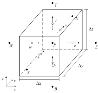
4.2 Elementary control volume retained for the discretization of transport equations. 65
4.3 Non-uniform finite-volume grid and distances associated to the face e. . . 66
4.4 Evolution in physical and scalar sample spaces of notional particles are subject to Eqs. (3.72) and (3.73). . . 75
4.5 Evolution of the PDF of a illustrative case with particles subjected to Eq. (3.72) and Eq. (3.73). . . 76
4.6 Weighted interpolation scheme. The solid lines represent the control volume edges, and the dashed lines connects the nodes and a particle p. . . 80
4.7 Distribution of the progress variable ˜c in the plane xz at t = 0.03 s (3000 iterations) (a) Finite Volume method (b) Monte Carlo method. . . 85
4.8 Distribution of the variance of the progress variable ˜c in the plane xz at
t = 0.03 s (3000 iterations) (a) Finite Volume method (b) Monte Carlo method. 85
4.9 Assessment on the consistency of the particle scheme: Solid line stands for the Eulerian (constant) density. The dashed line represents the instantaneous value of the density evaluated from the particle density control algorithm, and the dots are the time-averaged value of the density evaluated by such algorithm. 86
4.10 Equivalence between the method of finite volumes and the Monte Carlo method. Time-averaged value of the mean value of the progress variable for different positions along the computational domain. z∗
=z/δm is non-dimensionalized
based on the initial width of the mixing layer. . . 86
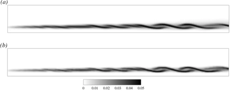
4.12 Two-dimensional temporal mixing layer simulation results for a density ratio
s = 2 at t∗
=tUr/Lr = 54. Contours of the scalar c. The figure in the right
hand side presents results for the simulation using the finite volume scheme. In the left hand side, results of the Monte-Carlo simulation. . . 88
4.13 Two-dimensional temporal mixing layer simulation results for a density ratio
s = 2 at t∗
= tUr/Lr = 50, where t is the physical time. Contours of the
variance of the scalar c. The figure in the right hand side presents results for the simulation using the finite volume scheme. In the left hand side, results of the Monte-Carlo simulation. . . 89
4.14 Time average results for the two-dimensional temporal mixing layer simulation for a density ratio s = 2 for number of particles per control volume Np equal
to 50 and 250. Left hand side: scalar quantity c, right hand side: its variance. 90
4.15 Instantaneous probes characterizing the equivalence between the Eulerian and Lagrangian approaches for different ratios of density Top to bottom: s = 2,
s = 4 and s = 8. From left to right: the value of the scalar quantity, its variance and the density variations along the z∗
axis. . . 91
5.1 Domain decomposition in a three-dimensional cartesian topology. N px, N py
and N pz stand for, respectively, the number of processes in the x, y and z
directions . . . 93
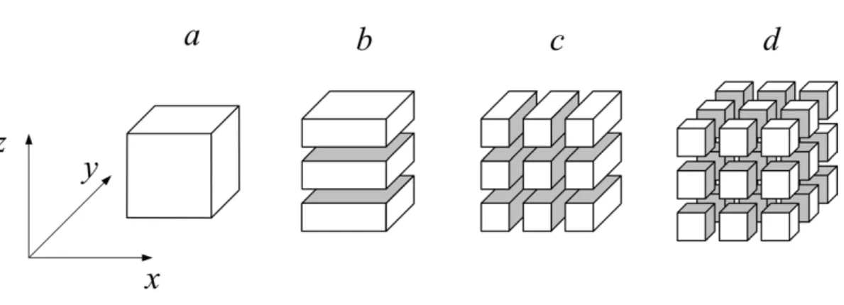
5.2 Domain decomposition in a cartesian topology. a) Original (serial) domain, b) one-dimensional decomposition, c) two-dimensional andd) domain decom-position in the three cartesian directions. . . 94
5.3 Domain decomposition in a one-dimensional cartesian topology and data ex-change scheme for vectorial and scalar variables. . . 97
5.5 Reallocation of pointers in the process of deleting an node in a linked list. The arrows departing for the pointers “prev” and “next” indicate the previous and next data members. . . 100
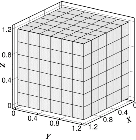
5.6 Original domain sub-divided in 216 sub-domains. Each cubic box of the as-sembling is assigned to a processor (core). . . 105
5.7 Speed-up evaluation for the hybrid finite-volume Monte-Carlo method. . . . 106
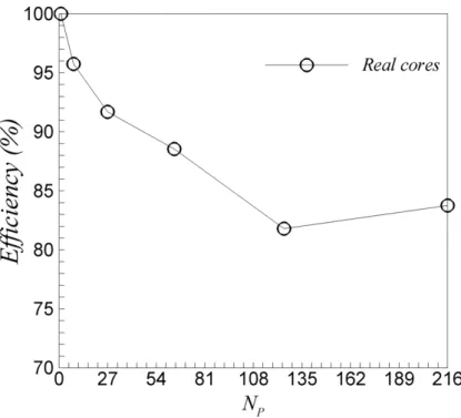
5.8 Efficiency of the parallel implementation of the hybrid finite-volume Monte-Carlo method. . . 108
6.1 Decay of the L2 norm for the zero Mach number manufactured solution with
Dirichlet boundary conditions. : u, N: v, : w, H: c, •: p. The solid line stands for the second order decay rate, and the dashed line stands for first order decay rate. Left figure: CDS approach; right: deferred correction approach. . . 116
6.2 Decay of the L2 norm of the zero Mach number manufactured solution with
mixed boundary conditions. : u, N: v, : w, H: c, •: p. The solid line stands for the second order decay, and the dashed line stands for first order decay. Left figure: CDS approach; right: deferred correction approach. . . 117
6.3 Evolution of the density field. The isolines stand for equally spaced density levels. . . 120
6.4 Evolution in time of the L2 norm. . Left figure: s= 5; right: s = 7. : u, N:
v, : p, •: c, ◮:ρ. The solid line stands for the second order decay, and the
dashed line stands for first order decay. . . 122
6.5 Evolution in time of the L2 norm, s = 10. Single cycle (left), Two cycles
(right). : u,N: v,: p,•:c,◮:ρ. The solid line stands for the second order
7.1 Sketch of the rescaling/recycling method of Lund et al. (1998) (LUND, 1998) to generate inlet conditions for a zero pressure gradient boundary layer. . . . 129
7.2 R13component of the Reynolds stress tensor as a function of the non-dimensional
width of the mixing layer ξ, (BRUCKER; SARKAR, 2007). . . 138
7.3 Mean velocity profile imposed. z∗
=z/δm,δm is the initial width of the mixing
layer . . . 139
7.4 Energy spectra associated to a white noise. . . 141
7.5 Stress tensor components evaluated from the superposition of white noise over the mean velocity profile. . . 142
7.6 Comparison of the effects of size of the support (N) on the energy spectra in the method of Klein, Sadiki and Janicka (2003). . . 143
7.7 Stress tensor components evaluated from the method of Klein, Sadiki and Janicka (2003), for different sizes of filter support. . . 144
7.8 Stress tensor components evaluated using the method of Smirnov, Shi and Celik (2001), for different numbers of Fourier modes. . . 146
7.9 Comparison of the effects of number of Fourier modes in the energy spectra in the method of Smirnov, Shi and Celik (2001). . . 147
7.10 Computational domain used for the simulations of the non-reactive flows. . . 148
7.11 Temporal evolution of the u component of velocity immediately downstream of the flow inlet; (a) White noise, (b) method of Klein, Sadiki and Janicka (2003) and (c) method of Smirnov, Shi and Celik (2001). . . 149
7.13 Fluctuations of √R11 for the simulations carried-out with: (a) White noise,
(b) method of Klein, Sadiki and Janicka (2003) and (c) method of Smirnov, Shi and Celik (2001). . . 150
7.14 Turbulent kinetic energy, k∗
=k/U2
r, for the simulations carried-out with the
method: (a) White noise, (b) , method of Klein, Sadiki and Janicka (2003) and (c) method of Smirnov, Shi and Celik (2001). . . 151
7.15 Snapshot of the normalized effective turbulent viscosityµ∗
ef f ec att
∗
= 586, for the simulations carried-out with the method: (a) White noise, (b) method of Klein, Sadiki and Janicka (2003) and (c) method of Smirnov, Shi and Celik (2001). . . 152
7.16 Perspective, top and lateral views of the isosurface of the second invariant of the velocity-gradient tensor Q = 26, at t = 0.020 s. The method of Klein,
Sadiki and Janicka (2003) was used. . . 153
7.17 Mean longitudinal velocity profiles. (•): Moreau and Boutier (1977); method of Smirnov, Shi and Celik (2001) (- - -); method of Klein, Sadiki and Janicka (2003) (− · −); white noise (− · ·−). . . 154
7.18 √R11 stress tensor component. (•): Moreau and Boutier (1977); method of Smirnov, Shi and Celik (2001) (- - -); method of Klein, Sadiki and Janicka (2003) (− · −); white noise (− · ·−). . . 154
7.19 Turbulent kinetic energy. Method of Smirnov, Shi and Celik (2001) (- - -); method of Klein, Sadiki and Janicka (2003) (− · −); white noise (− · ·−). . . 155
7.21 Instantaneous fields of chemical reaction progress variablec- left, and chemical reaction rate S(c) - right. (i) −Ea = 8,000 J/mole; (ii)−Ea = 10,000
J/mole; (iii) −Ea = 12,000 J/mole. The subfigures (a), (b) and (c) are
results of simulations with the respective inlet boundary condition methods: white noise superimposition; the method of Klein, Sadiki and Janicka (2003) and the method of Smirnov, Shi and Celik (2001) . . . 160
7.22 Average fields of chemical reaction progress variable c - left, and chemical reaction rate S(c) - right. (i) −Ea = 8,000 J/mole; (ii)−Ea = 10,000
J/mole; (iii)−Ea = 12,000 J/mole. The subfigures (a), (b) and (c) are results
of simulations with the respective inlet boundary condition methods methods: white noise superimposition; the method of Klein, Sadiki and Janicka (2003) and the method of Smirnov, Shi and Celik (2001) . . . 161
7.23 Instantaneous fields of chemical reaction rate (a) and chemical reaction progress variable (b). The isosurface presented in Fig. (7.23) is associated with a value of c= 0.5. . . 163
7.24 Evolution of the longitudinal average (top) and RMS (bottom) of the u -component of velocity at the centerline of the channel. . . 164
7.25 mean temperature profile at x= 42 and x= 122 mm. . . 165
8.1 Experimental configuration of the turbulent bunsen burner of Chen et al. (1996).167
8.2 Location of the flames studied by Chen et al. (1996) in the combustion regime diagram (Borghi coordinates) for premixed turbulent combustion. . . 168
8.3 Normalized mean and RMS velocity profiles at the burner exit plane, from Chen et al. (1996). . . 169
8.4 Scalar variable boundary condition at the computational inlet for the round jet. Global and detailed view of the jet region. . . 170
8.6 Streamwise evolution of average velocity and kinetic energy profiles for the cold jet. . . 172
8.7 Radial variation of average velocity and kinetic energy profiles for the cold-flow F3 jet. The solid lines are results of the present thesis, the plus, (+), symbols are numerical results obtained by Yilmaz (2008) and the circles are experimental results of Chen et al. (1996). . . 173
8.8 Instantaneous fields of the chemical reaction progress variablec, and the chem-ical reaction rate S(c) at t∗
= 22.5. . . 175
8.9 Instantaneous chemical reaction progress variable fields for t∗
= 0 until t∗
= 22.5. The non-dimensional time interval between figures is t∗
5.1 Numerical efficiency and speed-up factor evaluation for various topologies of parallelization. . . 107
6.1 Obtained convergence rates for Dirichlet boundary conditions and CDS ap-proach for the spatial discretization of the advective terms. . . 115
6.2 Obtained convergence rates for Dirichlet boundary conditions and deferred-correction approach for the discretization of the advective terms. . . 115
6.3 Obtained convergence rates for mixed boundary conditions and Central dif-ferencing scheme for the advective terms. . . 116
6.4 Obtained convergence rates for mixed boundary conditions and deferred-correction differencing scheme for the advective terms. . . 117
6.5 Values of the constant parameters for the variable density numerical simula-tion. . . 119
6.6 Obtained convergence rates for low Mach number solution, s =ρ0/ρ1 = 2. . . 121
6.7 Obtained convergence rates for low Mach number solution, s =ρ0/ρ1 = 5. . . 121
6.8 Obtained convergence rates for low Mach number solution, s =ρ0/ρ1 = 7. . 121
6.9 Obtained convergence rates for low Mach number solution, s =ρ0/ρ1 = 10. . 123
6.10 Obtained convergence rates for low Mach number solution, s = ρ0/ρ1 = 10,
two cycles per iteration. . . 124
7.1 Constant values used for mean velocity profile. . . 140
7.2 Values for mean velocity profile retained for the simulation of reactive flows. See Eq. (7.21) . . . 157
7.3 Procedure to evaluate the chemical source term. . . 159
7.4 Length of the 2D flame brush, based on hci= 0.9 in the x direction. . . 160
Abbreviations
BDF - Backwards Differencing Scheme
BICGST AB - Bi-Conjugate Gradient Stabilized
BM L - Bray, Libby and Moss combustion model
CD - coalescence and dispersion micro-mixing model
CDS - Central Differencing Scheme
CGD - Counter Gradient Diffusion
CF L - Courant Friedrich Lewy criteria
CP U - Central Processing Unity
CV - Control Volume
DN S - Direct Numerical Simulation
F DF - Filtered Probability Density Function
F GT - Flame Generated Turbulence
F V - Finite Volume Method
IC - Internal Combustion
IEM - Micro-mixing model - Interaction by Exchange with the mean
GD - Gradient Diffusion
LES - Large Eddy Simulation
LM SE - Linear Mean-Square Estimation micro-mixing model
M CN - Modified Crank Nicolson method
M M S - Method of Manufactured Solutions
M P I - Message Passing interface
M SIP - Modified Strongly Implicit Procedure
ODE - Ordinary Differential Equations
P DE - Partial Differential Equations
P DF - Probability Density Function
P GS - Pressure Gradient scaling
RAN S - Reynolds Averaged Navier Stokes Equations
RM S - Root Mean Square
RF G - Random Flow Generator
SDE - Stochastic Differential Equations
SGS - Subgrid scale
U DS - Upwind Differencing Scheme
U RAN S - Unsteady Reynolds Averaged Navier Stokes Equations
Greek
α - thermal diffusivity
β1 - exponent of temperature of the Arrhenius law
δij - Kroenecker delta
δm - width of the mixing layer
δj - initial width of the shear layer in the jet flow
∆ - filter width in LES
∆min - total mass entering each computational volume at each time step
∆x, ∆y, ∆z - respectively, the mesh discretization length in the x, y and z directions ∆t - size of time step
η - Kolmogorov length scale
ε - kinetic energy dissipation
γs - strong order of convergence
γw - weak order of convergence
Γ - molecular diffusivity
Γk - molecular diffusivity of the chemical speciek
λ - thermal conductivity of the fluid Λ - flame parameter
µ - dynamic viscosity
µef - effective turbulent viscosity
µm - m-th central statistical moment
µSGS - subgrid (or turbulent) viscosity
ν - kinematic viscosity
ρ - density
τc - Chemical time scale
τη - Kolmogorov time scale
τij - viscous strain rate tensor
τSGS
ij - subgrid scale (SGS) stress tensor
φ - generic scalar
Φ - joint scalar-velocity vectorial fields
ψ - sample space of the mass fractions of the chemical species Ψ - sample space of the scalar field
Ψα - sample space of theα scalar field
Ωm - turbulent frequency determined by LES
˙
ωF - rate of fuel consumption
Latin
aij - transformation matrix based on the Cholesky decomposition
Aτ - pre-exponential constant of the Arrhenius law
c - Chemical reaction progress variable
cq - mean values of the progress variable of the auxiliary burner
cp - mean values of the progress variable of the main duct
Cp - mean specific heat at constant pressure of mixture
CS - Smagorinsky constant
Cω - mechanical-to-scalar time-scale ratio
❣
c”2 - variance of the scalarc
D - nozzle diameter
Da - Damk¨oler number
dW(t) - increment of the Wiener process
DN o - square of the distance between a particle and a node N o
Ea - activation energy
E(k) - Energy spectrum as a function of wave number
Etot
n - efficiency of the parallelization
F - filter function
h - characteristic mesh size in the MMS
hk - specific enthalpy of the chemical speciek
Jhj - molecular flux of enthalpy in thej direction
Jkj - molecular flux of thek chemical specie in thej direction
K - number of chemical species
Ka - Karlovitz number
Kaδ - Karlovitz number based on the inner layer of the premixed laminar flame
k - Turbulent kinetic energy or wave number
l - integral length scale
lF - laminar flame front thickness
lδ - thickness of the internal layer of laminar flame
Le - Lewis number
Lek - Lewis number of the chemical speciek
M a - Mach number
m(l) - mass of a particlel
mF V - mass of fluid in a finite-volume cell of volumeVc
mpc - sum of mass of all particles in the cell of volumeVc
Mk - molar mass of chemical species
NB - Bray number
Np - number of particles in a finite-volume cell
N px, N py, N pz - respectively, the number of processes in the x,y and z directions
Nx, Ny,Nz - respectively, the filter support size along the directionsx, y, z
Po(t) - thermodynamic pressure, a function of time only
P r - Prandtl number
p - pressure
q - convergence rate
Qαj - subgrid scale (SGS) scalar flux
R - universal gas constant
Rij - Reynolds stress tensor components
Rj - Jet radius
re - error decay ratio
Re - Reynolds Number
Ro - mixture gas constant
R - set of independent random numbers
Ru,i - set of independent random numbers with zero mean and unity
s - density ratio
Sin - inflow surface area
Sn - speed-up factor
SL - laminar speed of a premixed flame
Sh - source term of enthalpy
S(c) - filtered chemical reaction rate source term
Sui - represents the body forces in momentum equations
Sk - chemical reaction rate of the k-th species
Sc - Schmidt number
Sck - Schmidt number of the chemical specie k
ScSGS - subgrid Schmidt number
˜
Sij - strain rate tensor of the resolved field
Ta - activation temperature
tadv - maximum allowable size of time step due advective contributions
tdif - maximum allowable size of time step due diffusive contributions
tther - maximum allowable size of time step due thermal contributions
ts - execution time for the best serial algorithm on a single processor
tn - execution time for the parallelized algorithm usingn processors
t - time
T - temperature
Tb - temperature of burnt gases
Tu - temperature of fresh gases
Ur - mean velocity between the two flow streams in the mixing layer
uq - mean inflow velocity at the auxiliary burner
up - mean inflow velocity at the main duct
˜
uip - i-th component of the velocity vector interpolated at a particle
ui(x, t) - velocity components
Uin - average velocity normal to the inflow surface
u′
- velocity fluctuations
utau - hear velocity
ub
k - conditional velocities in burnt mixture
uu
k - conditional velocities in fresh mixture
Vc - Volume of a mesh element
vη - Kolmogorov velocity scale
x - spatial coordinates ˙
WF - mean reaction rate of fuel inside the flame front
1 INTRODUCTION 1
2 TURBULENT COMBUSTION MODELING 6
2.1 Turbulence and spatially developing free shear flows . . . 6
2.2 Compressible vs low Mach number approximations . . . 12
2.2.1 Density-based methods . . . 13
2.2.2 Pressure-based methods . . . 15
2.3 Turbulent premixed combustion modeling . . . 17
2.3.1 Large Eddy Simulation . . . 18
2.3.1.1 Characteristic turbulent time, velocity and length scales . . 22
2.3.2 The laminar premixed flame . . . 23
2.3.2.1 Thickness and velocity of a laminar premixed flame . . . 24
2.3.3 Regimes and diagram of premixed turbulent flames . . . 24
2.3.4 Effects of flame fronts on turbulence . . . 26
2.3.5 Combustion models . . . 28
3 MATHEMATICAL MODELING 31
3.1 Governing equations . . . 32
3.1.1 Filtered transport equations . . . 35
3.1.2 Subgrid closure: the Smagorinsky Model . . . 37
3.1.3 Subgrid closure: the dynamic Smagorinsky Model . . . 38
3.1.4 Subgrid closure: the scalar flux . . . 40
3.1.5 Chemical reaction rate . . . 41
3.1.6 Simplifying assumptions of the chemical kinetics . . . 42
3.2 Turbulent combustion modeling using a Hybrid LES/PDF computational model 46
3.2.1 Transport of the Probability Density Function . . . 47
3.2.1.1 Joint velocity-scalar PDF . . . 48
3.2.1.2 Joint scalar PDF . . . 50
3.2.2 Lagrangian Monte Carlo approach . . . 54
3.2.3 Coupling of the hybrid model solvers . . . 56
4 NUMERICAL MODELING 58
4.1 The finite volume method . . . 59
4.1.1 Temporal approximations and numerical stability . . . 61
4.1.2 Variable time step size approach . . . 62
4.1.3 Spatial discretization of the transport equations . . . 65
4.2 Pressure velocity coupling . . . 68
4.2.1 A physically consistent constraint over the velocity field . . . 68
4.3 Numerical modeling of the system of stochastic differential equations . . . . 71
4.3.1 Method of fractional steps applied to the solution of SDE’s . . . 72
4.3.2 Operator splitting . . . 75
4.3.4 Numerical aspects associated to the lagrangian Monte Carlo approach 78
4.3.4.1 Initialization of the particle field . . . 79
4.3.4.2 Interpolation of average eulerian quantities to the particle field 79
4.3.4.3 Particles weighting control . . . 80
4.3.4.4 Estimation of average quantities from particle fields . . . 82
4.4 Equivalence between Eulerian and lagrangian approaches . . . 82
4.4.1 Scalar field results for constant-density flows . . . 83
4.4.2 Scalar field results for variable-density flows . . . 87
5 PARALLEL APPROACH 93
5.1 The finite-volume method parallelization . . . 96
5.2 Parallelization of the Lagrangian approach . . . 98
5.2.1 Data structure and linked lists . . . 99
5.2.2 Data exchange between sub-domains . . . 100
5.3 Performance assessment on the parallel approach implemented. . . 103
6 CODE VERIFICATION 109
6.1 Verification of an incompressible solution . . . 113
6.1.1 Convergence rate analysis . . . 114
6.2 Verification of the low-Mach number solution . . . 118
6.2.1 Convergence rate analysis . . . 120
7 TURBULENT INLET CONDITIONS 126
7.1 Recycling methods . . . 128
7.2.1 White noise based synthetic turbulence generators . . . 130
7.2.2 Digital filters based synthetic turbulence generator . . . 132
7.2.3 Synthetic turbulence generators based on Fourier techniques . . . 134
7.2.4 Assessment of the capability for reproducing prescribed Reynolds stress tensors . . . 137
7.2.4.1 White noise generator . . . 140
7.2.4.2 The method of Klein, Sadiki and Janicka (2003) . . . 142
7.2.4.3 The method of Smirnov, Shi and Celik (2001) . . . 145
7.2.5 Non-reactive flow simulations . . . 147
7.2.6 Application to reactive flows simulations . . . 156
7.2.6.1 Three-dimensional simulations . . . 162
8 APPLICATION TO NON-REACTIVE AND REACTIVE HIGH
VELOC-ITY TURBULENT JET OF PREMIXED REACTANTS 166
8.1 Cold-flow characteristics . . . 168
8.2 The turbulent Bunsen flame F3 . . . 174
INTRODUCTION
The presence of turbulent flows in practical engineering applications is very frequent, as well as the presence of reactive flows. However, the detailed analysis of these phenomena (turbulence and combustion), and especially the interaction between them is an area that still requires research and understanding. Combustion is a phenomenon that came to mankind since time began, and now, much of the energy used comes from combustion processes. Ac-cording to Turns (2000), in 1996, 85% of energy use in the U.S., came from combustion sources. In Brazil, as reported by the Ministry of Mines and Energy in 2006 over 80% of energy generated by human beings is related to some process of combustion. This reason alone is enough to motivate scientific research looking for maximum efficiency of any process involving combustion, however, such a dependency also leads to a major source of problems: environmental pollution. Most of the pollutants produced by total or partial combustion of fuels are hydrocarbons, nitrogen (N Ox) and sulfur (SOx) oxides, carbon monoxide and
particulate, are highly toxic and therefore its production has been increasingly regulated and restricted.
the prediction and understanding of such a category of flows, the extensive use of mathe-matical and numerical techniques is unavoidable. Hence, as the mathemathe-matical and numerical methods become more complex. This project aims to develop the understanding of the in-teraction between turbulence and combustion, through computational simulations of both processes by the joint use of adequate mathematical models and numerical tools to deal with the turbulent combustion in low Mach number flows.
Figure 1.1: A 400MW gas turbine, http://www.global-greenhouse-warming.com/gas-as-a-wedge-against-carbon-emissions.html, accessed on 16/08/2011.
The development of a numerical platform, aiming the numerical simulation of low Mach number turbulent premixed combustion, is the main subject of the present thesis. Adequate and robust methods for dealing with this kind of flows, where strong variations of density may came from temperature variations, reliable turbulence modeling, verified and accurate numerical methods, correct imposition of boundary conditions for large eddy sim-ulations and stochastic methods for modeling chemical reactions and mixture in turbulent combustion are examples of themes studied in the present work. These knowledge areas have received special attention recently for, at least, one reason in common: as we advance in terms of mathematical modeling, i.e. as the physical problems will be better understood, the computational cost of such methods typically increases, either by more complex models or due its need for increasingly refined meshes, hence the use of distributed computing is unavoidable.
about the methods retained for the modeling of turbulent combustion. Moreover, in the same chapter it is presented the main characteristics of the flows studied here, spatially de-veloping free shear flows. Chapter 3 reports a detailed description of the whole mathematical modeling retained, i.e., the governing transport equations, as well as the filtering procedure used for the obtention of a set of equation suitable for LES. The turbulence closures re-tained are also shown in chapter 3. Finally in this chapter, the simplificative assumptions of the chemical kinetics, a detailed demonstration of the transported PDF method used in the present work, and the coupling between the Eulerian and Lagrangian approaches is presented.
In chapter 4 the fully implicit discretization and the variable time-step temporal inte-gration of the finite volume approach retained is presented. The pressure velocity coupling and the physically consistent constraint developed for variable density flows are reported in detail also. Finally, the numerical approach used in the solution of the system of stochastic differential equations (SDE) generated is explained and its consistence with the Eulerian approach is proved for both constant density and variable density flows. Since it is intended to perform large eddy simulations of complex flows, the number of control volumes used to discretize the transport equations can be larger than one million and the number of notional particles retained in the solution of SDEs can amount to over hundreds of millions, the use of distributed computing is mandatory. Chapter 5 is devoted to describe the procedures retained in the parallelization of the aforementioned methods. The speed-up factor and ef-ficiency tests show that the approach implemented is very promising.
results showed that the numerical methods implemented has achieved a convergence rate of error decaying equals to two, allowing us to retain it to perform large eddy simulations of turbulent reactive flows.
The specification of the realistic turbulent inflow boundary conditions can be problem-atic in a LES context. The reason of that is due to the fact that for LES or DNS simulations, where the flow at the inlet is turbulent, the inflow data should consist of an unsteady turbu-lent velocity signal representative of the turbulence at the inlet. In Chapter 7 three different methods of prescribing turbulent inflow data are assessed and their effects are analyzed for a spatially developing mixing layer.
TURBULENT COMBUSTION MODELING
The objective of the present chapter is to present a very short survey of the literature concerning the methods retained in the computational modeling of turbulent reactive flows. Furthermore, are presented the main characteristics of spatially developing free shear flows, such as mixing layers and jets, the two main types of flows studied in the present thesis. The existing strategies that are usually employed to develop compressible and incompressible solvers for low Mach number calculations are briefly reviewed, as are the methods retained in the modeling of turbulent reactive flows. The text focuses, then, on the physical phenomena that involve the modeling of turbulent premixed flames, and the possible approaches that can be retained for the simulations of such flames.
2.1 Turbulence and spatially developing free shear flows
Although a definition that comprises all characteristics of turbulence is hardly ac-ceptable (SILVEIRA-NETO, 2002), it can be said that turbulence is a three-dimensional, rotational, highly diffusive, highly dissipative, unpredictable phenomenon that occurs at high Reynolds numbers. Such a set of characteristics associates the turbulence in fluids to a highly non-linear character. Moreover, turbulent flows present a wide energy spectra, i.e., in tur-bulent flows there are structures with different wave numbers, and the interactions between these different structures with characteristic sizes and frequencies constitutes a refined and complex mechanism of energy transfer.
Figure 2.1: Flow visualization of a plane mixing layer between helium (upper) and nitrogen (lower) (BROWN; ROSHKO, 1974).
vorticity absorbed by adjacent eddies (POPE, 2000).
Brown and Roshko (1974) and Browand and Latigo (1979) developed pioneering works in the sense of a full experimental characterization of mixing layers. Soteriou and Ghoniem (1995) assessed the effects of free-stream density ratio on low-Mach number developing mix-ing layers. Direct Numerical Simulations of a temporally evolvmix-ing shear layer has been performed by Brucker and Sarkar (2007). An important contribution of such a work is that they present a relation in which the non-dimensional thickness of the shear layer is corre-lated to parcels of the Reynolds stress tensor. Moreover, in Brucker and Sarkar (2007) the influence of turbulent initial conditions on the development of self-similar mixing layers is assessed.
Figure 2.2: CO2 round jet entering air at Re = 30,000. The instabilities developed
down-stream the nozzle and rapidly become completely turbulent (LANDIS; SHAPIRO, 1951).
classi-fied according to the geometry of the nozzle. In a planar jet, for instance, the nozzle has a rectangular format, whereas a round jet is formed downstream of a circular nozzle. In both cases the transition to turbulence is characterized by the formation of Kelvin-Helmholtz-type primary instabilities, which induce the generation of secondary longitudinal filaments. The interaction of such secondary counter-rotating longitudinal filaments with the primary eddies leads to the formation of transversal oscillations. The latter are amplified and eventually lead the flow to a state of developed turbulence. The primary instabilities are easily notable in Fig. (2.2).
The first investigations on jets include the work of Corrsin (1943), Corrsin and Uberoi (1950a, 1950b). Considering its applicability in several areas of engineering, it is natural that numerous publications analyze turbulent jets from different points of view. Heron et al. (2001), Birch et al. (2003) and Uzun (2003) studied compressible jets in order to understand the interactions between aerodynamic and acoustic noise generation. Hussein, Capps and George (1994) have studied round incompressible jets at high Reynolds numbers, showing that averaged velocity, second, and third order statistical moments depend strongly on the experimental set-up. In the work of Todde, Spazzini and Sandberg (2009) a series of com-mon characteristics of jets at low and moderate Reynolds numbers are evidenced, e.g., the presence of eddies near the nozzle and the existence of the shear layers. Todde, Spazzini and Sandberg (2009) also evidenced and characterized the presence of a potential core in turbulent non-reactive jets.
the jet develops downstream. In fact, higher intensity fluctuations lead to a faster growth of the jet with an asymptotic approach of the centerline turbulent kinetic energy to self-similar values. Xu and Antonia (2002) experimentally examined the effects of the velocity profile at the nozzle on the development of a turbulent round jet. They found that the use of a smooth contraction, leading to a top-hat type profile, leads to a faster jet development to a self-similar behavior than when the flow issues from a long tube, characterized by a velocity profile of a fully developed pipe flow.
The application of Large Eddy Simulations in the study of turbulent non-reactive jets is also a subject of numerous works. Silva and M´etais (2002), by using an compact sixth-order scheme in the direction of the development of the jet, and pseudo-spectral methods in the transversal directions, studied the dynamics and control of bifurcating jets, focusing on the analysis of the influence of forcing 1 and the Reynolds number.
Silva and Pereira (2004), simulating a jet in temporal decay, studied the effects of subgrid models in order to analyze the effect of the subgrid-scale (SGS) models on the vor-tices obtained from LES. The dynamics of the filtered vorticity norm (or filtered enstrophy) was analyzed through the application of a box filter to temporal DNS of turbulent plane jets. The models analyzed were the Smagorinsky, structure function, filtered structure func-tion, dynamic Smagorinsky, gradient, scale similarity, and mixed. Those model results were also compared with DNS results. Silva and Pereira (2004) showed that, in terms of spatial location, all the models used lead to a good correlation between the “real” and “modeled” enstrophy SGS dissipation. Moreover, all the SGS models, even of eddy-viscosity type, are able to provide enstrophy SGS backscatter. However, in terms of statistical behavior the eddy-viscosity models do not provide enough enstrophy backscatter when compared to the non-eddy-viscosity models. LES are carried out and show that the Smagorinsky, structure function, and mixed models cause excessive vorticity dissipation, compared to the other models, and, although the enstrophy SGS dissipation affects mainly the smallest resolved scales, it is argued that it may also affect some low-wave numbers.
1
(a) (b)
(c) (d)
(e) (f)
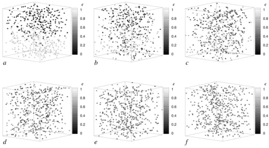
Figure 2.3: Temporal evolution of Q = 0,1 [s−1
] isosurfaces: (a) t=0.1 [s],(b) t=5 [s], (c) t=10 [s],(d) t=20 [s], (e) t=30 [s] e (f) t=40 [s]. (MOREIRA, 2011).
prob-lems to which the FPSM could be applied towards more complex probprob-lems. Figure (2.3) shows the temporal evolution of the criteria Q isosurfaces (JEONG; HUSSAIN, 1995) of a spatial developing jet at Re = 1,050. The first vortical structures of the Kelvin-Helmholtz instabilities are clearly identifiable.
So far, a brief overview of the literature concerning non-reactive free shear flows was presented. Before presenting how combustion chemical reactions may affect turbulent free shear flows, and how turbulent reactive flows have been treated in the scientific literature, an overview about the possible numerical methods that can be retained for simulating those kind of flows is given. The reason for this is due to the interest of the present thesis in flows that present non-negligible density variations, but are in a low-Mach number regime.
2.2 Compressible vs low Mach number approximations
An important non-dimensional parameter that characterizes a flow field is the Mach numberM a=U/c, where U is a characteristic velocity of the flow field, andcis the speed of sound. The incompressible limit is usually defined as the situation associated to Mach num-ber values smaller than 0.3. Above this value the compressibility effects cannot be neglected any longer, and variations of density and pressure are coupled through an equation of state. For incompressible flows a partial decoupling between the equations of momentum and the energy equation is possible, and in such flows the pressure variations are typically very small. The possible density variations are not related to pressure variations, but to temperature and mixture composition variations. The pressure is often said to be thermodynamically constant, and its influence is only felt through the spatial derivatives that appear in the momentum transport equation.
equations follows an hyperbolic behavior (ANDERSON, 1995), whereas in the low Mach number incompressible case, the velocity of sound waves are much higher than the fluid velocity, i.e.,O(U)≪O(c). Such a disparity of magnitudes between the velocity of the flow and the speed of sound waves leads to a great stiffness in the system of balance equations. This severely hampers the accuracy and convergence of the numerical methods that rely on the consideration of density variations, i.e., density-based solvers (CHOI; MERKLE, 1993), which remain the most commonly used to perform the numerical simulations of compressible flows. In the case of incompressible flows such a disparity between the wave and flow veloc-ities is also one of the major sources of numerical instability (NAJM; NAJIM; WYCKOFF, 1998; COOK; RILEY, 1996; RAUWOENS; VIERENDEELS; MERCI, 2007).
In the present work, the interest is focused on low velocity flows, i.e., in the incompress-ible regime, but featuring non negligincompress-ible density variations, the so-called low Mach number flows. There are basically two broad classes of numerical methodologies to deal with this kind of flows: those relying on density-based solvers, i.e., based on methods usually retained for compressible flows, and those relying on pressure-based solvers, such as those retained to perform the numerical simulation of incompressible flows. The application of each one of these two methodologies to low Mach number flows requires the introduction of several modifications and improvements, that are briefly summarized below.
2.2.1 Density-based methods
each time step to enforce the numerical stability of the numerical integration scheme, leads to prohibitively small time step values due to the prevailing influence of acoustic waves propagation. In the case of implicit methods such a disparity induces large differences in the characteristic eigenvalues of the algebraic system to be solved, which becomes ill-conditioned, leading therefore to extremely high-cost iterative solutions (ROLLER; MUNZ, 2000).
Two distinct sets of techniques have been proposed to achieve better convergence prop-erties of density-based solvers, in the limit of low Mach number flows: preconditioning and perturbation methods. Both techniques strive to minimize the stiffness of the algebraic sys-tem that results from the discretization of the balance equations.
The first technique pre-multiplies the temporal derivatives by a preconditioning ma-trix, whose choice is determined according to the problem to be analyzed (CHOI; MERKLE, 1993), thus leading to a new set of equations. As a consequence, the initial (stiff) system is altered. The technique essentially aims at re-scaling the characteristic eigenvalues with respect to the original system, so that eigenvalues of similar orders of magnitude can be obtained, leading to a better conditioned system (TURKEL; RADESPIEL; KROLL, 1997; TURKEL, 1992). The major drawback associated with preconditioning methods is that the governing equations are modified in terms of their mathematical nature due to the incorpo-rated transient term. The modified system of equations has only the steady-state solution in common with the original system and becomes, therefore, devoid of any physical transients. A second limitation is the failure of this methodology, in terms both of efficiency and ro-bustness, in the vicinity of stagnation points, where the characteristic eigenvectors become almost parallel (DARMOFAL; SCHMID, 1996). Furthermore, the design of general purpose pre-conditioners adequate for a large variety of physical problems remains far from being straightforward.
number, thus decoupling the acoustic waves from the equations, and replacing them with a set of pseudo-acoustic forms, where the wave velocities become the same order of magnitude as the fluid velocity. Such a procedure alters the velocity of the acoustic waves in order to allow the numerical integration to be performed with larger time steps (CHOI; MERKLE, 1993; ROLLER; MUNZ, 2000).
Other methodologies have been also developed for the purpose of considering density variations, such as the artificial compressibility methods, and the PGS (Pressure Gradient Scaling). The first, described, for instance in Ferziger and Peric (1996), has been successfully applied to the numerical simulation of reactive flows and, in particular, to describe the propa-gation of a planar turbulent premixed flame (DOURADO; BRUEL; AZEVEDO, 2004). The PGS method (RAMSHAW; O’ROURKE; STEIN, 1985; AMSDEN, 1989; WANG; TROUV´e, 2004; PAPAGEORGAKIS; ASSANIS, 1999) displays certain similarities to the perturbation methods, and it also acts on the pressure term that appears in the momentum equation. In this method the pressure gradient is multiplied by a factor 1/α2
P GS, whereαP GS is a constant
that amplifies the pressure variations. As a consequence, since the velocity of acoustic waves is decreased by a factorαP GS, the pressure variations are amplified by a factor α2P GS, thus,
improving the robustness of the numerical method as the Mach number tends towards zero (AMSDEN, 1989). Finally, it is worth adding that one reason for the use of the last two methods rely in the fact that they can be easily implemented within existing compressible solvers.
2.2.2 Pressure-based methods
In a first step, momentum equations are solved to obtain an estimated velocity field, based on a previous evaluation of pressure. The velocity field should be solenoidal, and this property is enforced by a subsequent projection step within the subspace of divergence-free vectorial fields. Such projection, which defines the corrector step, relies on the Hodge decomposi-tion theorem (CHORIN; MARSDEN, 1993). The pioneering works in this field (CHORIN, 1968; PATANKAR, 1980) have provided the basis for the development of several projection schemes that are still currently used. More specifically, the work of Patankar (1980), has led to a family of methodologies referred to as the SIMPLE (Semi-Implicit Pressure Linked Equations) approach, which undoubtedly remains the most widely used to obtain the solu-tion of incompressible flows.
As previously mentioned, in the low Mach number regime, the compressibility effects have a negligible influence on the momentum transport and the pressure is only a weak function of density. To prevent significant inaccuracies when performing the evaluation of pressure, it is usually divided into two distinct components:
P(x, t) =Po(t) +P
′
(x, t), (2.1)
where Po is a reference pressure level2, with Po(t)/Po = O(1), and P(x, t)/Po = O(M a2).
It is worth noting that Po(t) is often referred to as the thermodynamic pressure, whereas
P′
(x, t) is called the dynamic pressure since it is directly related to modifications of the velocity field.
Using such a decomposition, the thermodynamic pressure appears in the equations of state and energy conservation only, vanishing in the momentum equation. Since its gradient is zero everywhere, only the gradient of the dynamic pressure component remains. It is worth noting that this procedure significantly accelerates the convergence only if the pressure fluc-tuations remain sufficiently small.
Since one of the objectives of the present work is to provide guidelines for verification
2
and cross-checks of a recently developed incompressible code, the most natural choice for an extension to variable density flows is a formulation based on pressure variations, i.e., to extend a mathematical and numerical model proposed for fully incompressible flows to handle density variations.
A wide class of numerical methods that remains used to perform such simulations of low Mach number flows, is based on predictor-corrector methods. Several works, (NAJM; NAJIM; WYCKOFF, 1998; COOK; RILEY, 1996; RAUWOENS; VIERENDEELS; MERCI, 2007; COLELLA; PAO, 1999; KARKI; PATANKAR, 1989; LIMA-E-SILVA; SILVEIRA-NETO; DAMASCENO, 2003; BELL, 2005a; LESSANI; PAPALEXANDRIS, 2006a; KNIO; NAJM; WYCKOFF, 1999) share such pressure-velocity coupling. Rider et al. (1998) report an extensive discussion about robust projection methods applied to variable density low Mach number flows. The details of the algorithm retained for the present study will be presented in Chapter 4. In the next sections a brief review on the modeling of turbulent combustion is presented.
2.3 Turbulent premixed combustion modeling
2.3.1 Large Eddy Simulation
As mentioned in the introduction of this thesis, the solution of the balance equations (mass, momentum, energy, species mass fractions, etc.) is deemed sufficient to represent the evolution of a multi-component gas-phase mixture in either laminar or turbulent flow, provided that the continuum hypothesis holds, and once suitable constitutive equations for the fluids of interest are specified (HAWORTH, 2010a). The full solutions of this set of equations is, however, far from being straightforward, specially under turbulent conditions. To solve each and every scale of a turbulent reactive flow, i.e., to perform a Direct Numer-ical Simulation of a turbulent reactive flow with the computational power available today still remains out of reach for problems of engineering interest, see for instance Pope (2000). Since all length and timescales must be resolved, the computational cost of a DNS increases proportionally to Re3, whereRe is the Reynolds number (POPE, 2000).
The highly non-linear set of PDE’s is extremely sensitive to small variations of initial and boundary conditions. If the simulation of an actual combustion device is of interest, in-formation on the boundary conditions is seldom available with the required level of accuracy. Moreover, the mesh required for the DNS simulation of reactive flows must be fine enough to resolve the inner structure of the flame, which, in many cases, is much smaller than the so-called Kolmogorov scales of the flow (POINSOT; VEYNANTE, 2005; HAWORTH, 2010a).
To give an idea of the computational cost of a DNS, Poinsot and Veynante (2005) present the results of a DNS of a premixed flame front at atmospheric pressure interacting with isotropic turbulence. The mesh adopted in a such simulation contains approximately two million grid points and the corresponding computational domain is a cubic box of size 5×5×5 mm3. Finally, even if a computation of full set of PDE’s of a turbulent reactive
flow is computationally possible, the large amount of data generated is too cumbersome to be dealt with for most practical purposes.
Reynolds Averaged Navier Stokes (RANS) or Unsteady Reynolds Averaged Navier Stokes (URANS) computations provide the temporal average of the flows properties of interest. Still largely adopted in turbulent combustion (POINSOT; VEYNANTE, 2005; FOX, 2003; HAWORTH, 2010a; YILMAZ, 2008), these methods consist on the application of a temporal average operator on the transport equations. Such a process results in averaged equations, with unclosed terms where some sort of closure is needed. These unclosed terms are the Reynolds stresses and the turbulent scalar fluxes, and the averaged chemical reaction term. Although indisputably much less expensive than DNS, providing mean values only precludes a RANS model from predicting turbulent structures that can influence the flame front, spe-cially in shear flows, such as mixing layers, boundary layers and jets (LIBBY; WILLIAMS, 1994).
The URANS methods also involve models for the unclosed terms in the turbulent transport equation for the scalar fields, such as the mass fractions and chemical reaction. The modeling of such terms in a URANS methodology is more complicated, due to the pos-sible occurrence of counter-gradient diffusion (LIBBY; BRAY, 1981).
Counter gradient diffusion can occur when the flow near the flame front is dominated by the acceleration induced by the thermal expansion due to the chemical reactions, whereas gradient diffusion occurs when turbulence dominates the flow field near the flame front. URANS models are usually based on gradient transport assumptions. This is an acceptable hypothesis in constant density flows, but in variable density flows, such an important phe-nomena, i.e. the counter gradient diffusion, cannot be accounted for within the framework of turbulent diffusion transport (YOSHIZAWA et al., 2009).
Large Eddy Simulations (LES) can be thought as an intermediate methodology be-tween the DNS and URANS. The large scales of the turbulent flows are explicitly calculated, whereas the non-linear interactions between large scales and subfilter scales are modeled us-ing subfilter (or subgrid) closure models. The balance equations for large eddy simulations are obtained by filtering the instantaneous transport equations. LES can determine the in-stantaneous position of a “large scale” resolved flame front but a subgrid model is required to account for the effects of small turbulent scales on the combustion processes (POINSOT; VEYNANTE, 2005). Since large structures are explicitly computed in LES, instantaneous fresh and burnt gases zones, where turbulence characteristics are quite different, can be, most often, clearly identified, at least at the resolved scale. In comparison with a URANS methodology, LES could provide a better prediction of the turbulence/combustion interac-tions. Schumann (1989) was one of the first to conduct a LES of a reacting flow. Colucci et al. (1998a) argue however, that the assumption made in that work, simply to neglect the contribution of the SGS scalar fluctuations on the filtered reaction rate, needs to be justified for general applications. The importance of such fluctuations is well recognized in Reynolds averaged procedures in both combustion and chemical engineering problems (LIBBY; WILLIAMS, 1994), therefore, it is natural to believe that these fluctuations are also important in LES.
cases, the arguments in favor of LES may be less compelling over RANS approaches, since the modeling of rate-controlling combustion on LES processes requires the same modeling as in RANS. In fact, most LES combustion models, with proper modifications, are derived from RANS models (FOX, 2003; POPE, 2004).
Figure 2.4: Axial swirler vanes and temperature iso-surface (T=1,000 K) colored by velocity modulus (SELLE et al., 2004).
along the burner axis by the recirculation zone induced by swirl (SELLE et al., 2004).
2.3.1.1 Characteristic turbulent time, velocity and length scales
Figure (2.5) shows the energy spectrum [E(k)] of homogeneous isotropic turbulence at a sufficient high Reynolds number, as a function of the reciprocal of the eddy size, i.e., the wave numberk. According to the Kolmogorov hypothesis (POPE, 2000), the energy transfer rate in the inertial subrange leads to a slope of−5/3.
Figure 2.5: Energy spectrum of a homogeneous, isotropic turbulence. Kinetic energy, [E(k)] as a function of wave number. Representation in a logarithmic scale.
Two important characteristic turbulent length scales bounding the inertial subrange can be identified in Fig. (2.5), the Kolmogorov length scale,η, and the integral length scale
l. The Kolmogorov length scales denotes the scale of the smallest eddies. At these length scales, dissipation of the energy due to viscous forces occurs. Thus, the Kolmogorov length scale has to be a function of the kinematic viscosity, ν, and the kinetic energy dissipation,
ε. In addition, the Kolmogorov time scale τη, can be defined as being proportional to the
turnover time of a Kolmogorov eddy. By dimensional analysis, the Kolmogorov length, time and velocity scales can be defined as,
η = ❶
ν3 ε
➀1/4
, τη =
r
ν
ε, vη =
⑨
ν3ε❾. (2.2)
are presented in the following sections. Such laminar parameters are important since, when compared to those of a turbulent flow in a flow regime diagram, the different regimes of premixed turbulent combustion can be identified. In the following section the regimes of premixed turbulent flames are presented.
2.3.2 The laminar premixed flame
In a qualitative way, the characteristics of a premixed laminar flame are now described using Fig. (2.6). The fresh gases enters at the left hand side at a temperature Tu and
are consequently burnt through the flame front. The burnt gases, at a temperature Tb, are
convected to the outlet (right hand side) of the domain of interest. If the injection velocity of the fresh gases is the same as the laminar flame speed, S0
l, such a flame front would appear
fixed to an external observer.
Figure 2.6: Evolution of the chemical reaction rate, temperature and mass fraction of fuel through a laminar flame front.
The flame front, with a thickness lF can be separated in two zones: a pre-heating
2.3.2.1 Thickness and velocity of a laminar premixed flame
Based on a one-dimensional analysis of the Navier-Stokes equations, supposing a cer-tain number of simplificative hypothesis (mainly supposing the flame as adiabatic and com-posed by gases with constant specific heat), Mallard and Chatelier (1883) procom-posed in 1883 to describe the laminar speed of a premixed flame as,
SL ∝
✏ ΓkW˙ F
✑1/2
, (2.3)
where ˙WF is the mean reaction rate of fuel inside the flame front3. Supposing the chemical
time,τc is of order 1/W˙ F, and considering thatlF ≈SLτc, it is possible to show that,
lF =
Γk
SL
, (2.4)
where, Γk is the molecular diffusivity of the chemical speciesk
2.3.3 Regimes and diagram of premixed turbulent flames
The understanding of the mechanisms by which turbulence and chemistry interact is essential prior to modeling of turbulent premixed combustion. Turbulent premixed reacting flows can be described by a wide range of characteristic time and length scales. The rel-evant turbulent and chemical time and length scales for laminar premixed combustion are important since, when compared to those of a turbulent flow in a flow regime diagram, the different regimes of premixed turbulent combustion can be identified. Borghi (1985) and Peters (1999), by analyzing experimental results of turbulent premixed flames, defined the possible modes of interaction between turbulent structures and flame structures. Such pos-sible interactions are based on the relations between the turbulent and combustion time and length scales. Thus, the combustion regimes, could be represented graphically by a diagram known as Borghi diagram, illustrated, in a logarithmic scale, in Fig. (2.7).
3
More precisely ˙WF =
1
Tb−Tu
❘Tb
Figure 2.7: Regime diagram for premixed turbulent combustion, adapted from Peters (1999). In the diagram presented in Fig. (2.7), the abscissa express the ratio l/lF, which can
be interpreted as a measure of the turbulent integral length scale,l, interacting with flames of thickness lF, lF being the total thickness of a laminar flame, proportional to the
thick-ness of the pre-heating zone. The thickthick-ness of the internal layer, where the majority of the chemical reaction occurs, is called lδ. The lδ is approximately of order 0.1lF. The ordinate
shows the ratio of u′
/SL, which is a measure of the turbulent intensity u′, over the laminar
flame speed SL. The line ReT = 1, with ReT = u′l/SLlF, (BORGHI, 1985) delineates the
turbulent combustion regime (ReT >1).
Considering the diagram shown in Fig. (2.7), at least four different turbulent premixed combustion regimes can be identified. They are outlined in the following.
1. Wrinkled flames regime: it is delimited by the condition of u′
/SL < 1. The laminar
flame velocity is higher than the intensity of fluctuations and, therefore, governs the process flame-turbulence interaction. The turbulence practically does not wrinkle the flame front. Since turbulence is desired in a number of industrial applications, this kind of flame has few practical applications (ANDRADE, 2009);
2. Corrugated flames regime: it is delimited by the conditions u′
/SL > 1 and Ka < 1,
where the Karlovitz number (Ka =l2
F/η2 =τc/τη), is the ratio between the chemical
PETERS, 1997). The characteristic turbulence intensity is higher than the laminar flame velocity, which induces the corrugation of the flame front. The smallest structures in the Kolmogorov scale however, are larger than the laminar flame thickness, thus not interfering with the internal structure of the flame;
3. Thin reaction zones: it is delimited by the conditions Ka > 1 and Kaδ = l2δ/η2 <1.
The first condition indicates that the Kolmogorov length scale, η, is smaller than the laminar flame thickness, lF. The second condition indicates that η is larger than
the inner layer of the laminar flame, lδ. In this case the turbulence could alter the
structure of the pre-heating layer of the flame and significatively modify the transport of the chemical species and energy. However, there still no interaction between the turbulence and the inner part of the flame;
4. Broken reaction zones or thickened flames: Above Kaδ > 1, with the Damkh¨oler
number, i.e., the ratio of the integral turbulence time scale to a characteristic chemical time scale, Da = τt/τc, smaller than 1, the turbulent length scale is sufficiently small
to penetrate the inner part of the laminar flame, lδ. It can promote local extinctions of
the chemical reaction due to heat and radicals losses in the pre-heating layer. In such a regime even a local extinction of the combustion is possible.
2.3.4 Effects of flame fronts on turbulence
The flame-turbulence interaction is a two-way mechanism. Turbulence not only af-fects the flame front, but the flame modifies the turbulent flow field also. An example of that occurs due the fact that when temperature changes along the flame front, kinematic viscosity and, therefore, the local Reynolds number changes as well. The kinematic viscosity of air, for instance, increases roughly asT1.7, which means that for a flame in which the ratio
Tb/Tu = 8, where Tb and Tu are the temperature of the burnt and fresh gases respectively,