Viscoelastic flow in a 3D square/square contraction: Visualizations and simulations.

Visualizations and simulations

M. A. Alvesa)

Faculdade de Engenharia da Universidade do Porto, Departamento de Engenharia Química, CEFT, Rua Dr. Roberto Frias, 4200-465 Porto, Portugal

F. T. Pinhob)

Centro de Estudos de Fenómenos de Transporte, Faculdade de Engenharia da Universidade do Porto, 4200-465 Porto, Portugal and Universidade do Minho,

Largo do Paço, 4704-553 Braga, Portugal P. J. Oliveirac)

Departamento de Engenharia Electromecânica, Unidade de Materiais Têxteis e Papeleiros, Universidade da Beira Interior, 6201-001 Covilhã, Portugal

(Received 1 December 2007; final revision received 26 August 2008兲

Synopsis

The inertialess three-dimensional 共3D兲 flow of viscoelastic shear-thinning fluids in a 4:1 sudden square-square contraction was investigated experimentally and numerically and compared with the flow of inelastic fluids. Whereas for a Newtonian fluid the vortex length remains unchanged at low Reynolds numbers, with the non-Newtonian fluid there is a large increase in vortex length with fluid elasticity leading to unstable periodic flow at higher flow rates. In the steady flow regime the vortices are 3D and fluid particles enter the vortex at the middle plane, rotate towards its eye, drift sideways to the corner-plane vortex, rotate to its periphery, and exit to the downstream duct. Such dynamic process is reverse of that observed and predicted with Newtonian fluids. Numerical predictions using a multimode Phan-Thien–Tanner viscoelastic model are found to match the visualizations accurately and in particular are able to replicate the observed flow reversal. The effect of fluid rheology on flow reversal, vortex enhancement, and entry pressure drop is investigated in detail. © 2008 The Society of Rheology. 关DOI: 10.1122/1.2982514兴

I. INTRODUCTION

Matching experiments and simulations in non-Newtonian flow systems is a matter of great relevance as illustrated in the recent study of Collis et al.共2005兲. It is useful to assess the adequacy of constitutive models and it may serve to explain or highlight new

a兲_{Author to whom correspondence should be addressed. Fax: ⫹351-225081449. Electronic mail:}

mmalves@fe.up.pt

b兲_{Electronic mail: fpinho@fe.up.pt; fpinho@dem.uminho.pt} c兲_{Electronic mail: pjpo@ubi.pt}

© 2008 by The Society of Rheology, Inc.

1347 J. Rheol. 52共6兲, 1347-1368 November/December 共2008兲 0148-6055/2008/52共6兲/1347/22/$27.00

fluid mechanics phenomena. In order to achieve these goals, it is necessary to select simple but useful flow geometries.

Sudden contraction flows are classical benchmark problems used in computational rheology关Hassager共1988兲;Brown and McKinley共1994兲兴 and possess features found in

many industrial situations, such as in extrusion processes. Consequently, a large number of experimental and numerical investigations can be found in the literature, although most are concerned with nominally two-dimensional共2D兲 planar and axisymmetric con-tractions 关e.g., Cable and Boger共1978a,1978b, 1979兲; Walters and Rawlinson 共1982兲;

Crochet et al.共1984兲;Evans and Walters共1986,1988兲;Boger et al.共1986兲;Boger共1987兲;

McKinley et al.共1991兲;Coates et al.共1992兲;Boger and Walters共1993兲;Quinzani et al. 共1994兲; Rothstein and McKinley共1999兲;Lee et al.共2001兲; Owens and Phillips共2002兲;

Walters and Webster 共2003兲; Alves et al. 共2004兲; Collis et al. 共2005兲; Oliveira et al. 共2007兲兴. In spite of the geometrical simplicity, the flow behavior of non-Newtonian fluids in contraction flows can be very surprising, and different flow patterns are observed even for fluids with similar rheological behavior 关Boger et al. 共1986兲; Owens and Phillips 共2002兲兴.

Studies related to three-dimensional 共3D兲 sudden contractions are less common, in spite of the practical relevance of this geometry, and the amount of published research on this topic has been scarce. The present work presents new experimental results based on flow visualizations, complemented with supporting results from numerical simulations, for Newtonian and viscoelastic shear-thinning fluids in a 4:1 sudden square/square共SQ/ SQ兲 contraction. In a previous investigation 关Alves et al.共2005兲兴, the behavior of Boger

fluids in the same geometry was visualized and a review of past work on the 2D planar and axisymmetric geometries was presented. Therefore, in this section we concentrate mainly on the 3D case.

To our knowledge, the first work on viscoelastic flows in 3D square contractions was published byWalters and Webster共1982兲who found similarities with the flow through a circular contraction. Walters and Rawlinson 共1982兲 also confirmed that the differences between the flows in planar and circular contractions also existed when comparing the flows in planar and the 13.3:1 SQ/SQ contractions. The experiments and numerical cal-culations of Purnode and Crochet共1996兲 confirmed the similarities between the main flow features in 2D and 3D flows, and they concluded that lip vortices should not be associated with inertial effects. However, these authors also found that full capture of 3D effects required 3D computations and especially an accurate representation of fluid rhe-ology.

As a precursor to the present contribution,Alves et al. 共2005兲carried out visualiza-tions with polyacrylamide-based Boger fluids in a 4:1 SQ/SQ geometry and found a nonmonotonic variation of the recirculation length with the flow rate. The corner vortex was found to increase initially共for one of the fluids兲, peaking at a Deborah number1 of around 6, followed by a strong decrease of length to a minimum at De2⬇15–20, for both

fluids analyzed. Then, as the Deborah number increased further the vortex length in-creased significantly until an unstable periodic flow was established at De₂⬇45 for the more concentrated Boger fluid and at De2⬇52 for the other. This increase in vortex

length was preceded by a divergence pattern of the streamlines, a typical behavior of Boger fluids related to their extensional properties, as discussed by Alves and Poole 共2007兲.

1_De

2=␭U2/H2, where U2and H2are the downstream channel bulk velocity and half side, respectively, and␭ is

Predictions of 3D contraction flows are scarce due to the large computational demands involved, but are in much need due to their relevance in practical situations.Mompean and Deville 共1997兲used a finite-volume methodology in a staggered grid to investigate the flow in a quasi-3D planar contraction, one that tends to become 2D when the aspect ratio is large enough, and compared qualitatively their results with the measurements of

Quinzani et al.共1994兲for a 4:1 2D planar contraction.

The 3D simulations of Xue et al.共1998a兲for upper-convected Maxwell共UCM兲 and Phan-Thien–Tanner 共PTT兲 fluids also employed a finite-volume method applied to a quasiplanar 4:1 contraction flow. For the corresponding 3D SQ/SQ contraction,Xue et al. 共1998b兲carried out a set of simulations with the same finite-volume method, using a PTT model having nonzero second normal stress differences and UCM constitutive equations. Vortex enhancement for both the constant viscosity and the shear-thinning viscoelastic fluids was found for both cases. In contrast, for the 2D 4:1 planar contraction only the PTT fluid exhibited vortex enhancement. These differences replicate those between axi-symmetric and planar contractions and result from the equivalent Hencky strains gener-ated in the circular and the SQ/SQ cases. This investigation concentrgener-ated on relating the flow dynamics with the transient extensional viscosity behavior of the fluids, but nothing was mentioned regarding secondary flows in the contraction region or the onset of flow instabilities.Xue et al.共1998b兲reported secondary flows in the fully developed upstream and downstream square duct flows for the case of PTT fluid, but these were exclusively due to nonzero second normal stress differences.

More recently, Sirakov et al.共2005兲studied the flow through 3D contractions using the eXtended Pom–Pom model; the geometry differed from the present one in that the exiting die was not a square duct but presented either a rectangular or a circular cross section. They found that the recirculation was an open vortex in which the fluid followed a complicated spiraling motion. More interestingly, for the square/circular contraction case, they noticed that the flow direction in the recirculation was reversed in the case of the viscoelastic fluid, as compared to the Newtonian case, a result which confirmed the previous observations ofAlves et al.共2003c兲for a SQ/SQ contraction.

It is clear that much remains to be known for the 3D SQ/SQ contraction and the increase in computational power over the last years has now made it possible to accu-rately perform numerical simulations of true 3D flows in reasonable time. This is the motivation for our work on SQ/SQ contractions and the present experimental and nu-merical work complements the previous experimental investigation ofAlves et al.共2005兲

who considered Boger fluids only. Here, visualizations and numerical predictions of the flow of a viscoelastic shear-thinning fluid in a 4:1 SQ/SQ contraction were carried out in much greater detail.

In the next section the experimental apparatus is briefly described and the results of the rheological measurements of the fluids are discussed. The numerical method and the constitutive equations used in the numerical solution are then briefly outlined in Sec. III and finally, in Sec. IV, results of the experiments and numerical simulations are presented and discussed in detail. The paper ends with the main conclusions of this work.

II. EXPERIMENTAL CONDITIONS A. Experimental rig

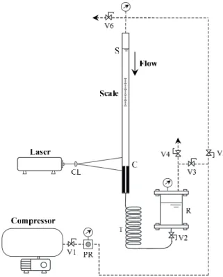
The experimental rig, schematically shown in Fig.1, was assembled as described in

Alves et al. 共2005兲, and the experiments were performed in a dark room. A 1000 mm long square duct having sides of 2H1= 24.0 mm was followed by a second 300 mm long

= H₁/H₂兲. The flow rate was set by an adequate control of applied pressure on the upstream duct 共dashed lines represent pressurized air lines, with applied pressures be-tween 0.5 and 4 bar兲 and frictional losses in the long coiled tube 共T兲 located at the bottom of the rig. The flow rate was measured by the stop-watch and level marker technique and the fluid temperature was monitored to properly take into account the fluid properties.

The flow was illuminated with a light sheet generated from a 10 mW He–Ne laser light source after the beam passed a cylindrical lens to create a sheet of light which illuminated highly reflective tracer particles suspended in the fluid 共10␮m PVC par-ticles兲. Their trajectories were recorded using long time exposure photography with a CANON EOS300 camera using an EF100 mm f/2.8 macrolens. For the smaller velocities very long exposure times were necessary 共above 1 h兲 and Hoya neutral-density filters were used 共ranging from 2⫻ to 400⫻ light transmittance reduction兲.

B. Rheological characterization of the fluids

The rheological properties of the viscoelastic fluids were measured by an AR2000 rheometer from TA Instruments with cone-plate geometry 共40 mm diameter and 2° angle兲. The shear viscosity 共␩兲 and the first normal stress difference coefficient 共⌿1兲 were

measured in steady shear flow, and the storage and loss moduli共G

⬘

⬙

Three fluids, listed in TableI, were investigated in this study: two viscous Newtonian fluids共N85 and N91兲 and a moderately shear-thinning viscoelastic fluid 共PAA500兲 made with polyacrylamide共Separan AP30 from SNF Floerger兲. The non-Newtonian fluid was

FIG. 1. Schematic representation of the experimental setup: C—contraction; CL—cylindrical lens; PR—

prepared by dissolving the required amount of PAA onto the Newtonian solvent of mod-erate viscosity共N85兲. To avoid bacteriological degradation the biocide Kathon LXE from Rohm and Haas was also added to all fluids at a concentration of 25 ppm. The fluid densities were measured at 294.4 K with a picnometer and are included in Table I.

For the N85 fluid the shear viscosity was␩= 0.125 Pa s at 291.2 K, the temperature at which the visualizations with this fluid took place, whereas for the N91 fluid the rheom-eter was used to measure the shear viscosity in the range of temperatures from 289.1 to 298.2 K. As described in Alves et al. 共2005兲, the effect of temperature on the viscosity was accounted for by the Arrhenius equation

ln共aT兲 = ln

冉

冊

冋

冉

冊

册

where T is the absolute temperature and T0is the reference absolute temperature. For the

N91 fluid, fitting of this equation to the experimental viscosity 共␩兲 data gave ⌬H/R = 6860 K and ␩0= 0.367 Pa s at T0= 293.2 K. More extensive measurements with fluid

N91 indicated a systematic uncertainty in the measurement of N1 of ⫾10 Pa and the

onset of inertial effects for␥˙⬎100 s−1_{which was well predicted by theory关Alves et al.} 共2005兲兴.

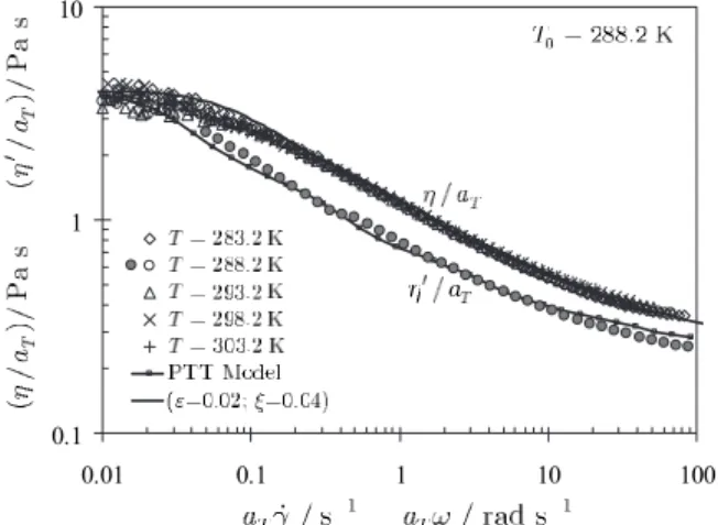
For the PAA500 solution, the dynamic measurements of the storage and loss moduli taken at 288.2 K allowed the determination of a linear viscoelastic spectrum. These are listed in TableII and the corresponding dynamic viscosity,␩

⬘

⬘

共lines兲 are compared with the experiments 共symbols兲 in Figs. 2 and3, respectively. We note that the solvent viscosity used in the fitting is somehow higher than the real shear viscosity of the solvent at the reference temperature. If we chose to match the Newtonian component of the shear viscosity to that of the base solvent we needed to use at least one more mode in the PTT model, otherwise predictions of G

⬘

⬘⬘

TABLE I. Composition of fluids in mass concentrations and density.

Designation PAA共ppm兲 Glycerin共%兲 Water共%兲 NaCl共%兲 Kathon共ppm兲 ␳共kg/m3_兲a

N85 — 84.99 15.01 — 25 1221

N91 — 90.99 7.51 1.50 25 1250

PAA500 500 84.97 14.98 — 25 1226

a_{Measured at 294.4 K.}

TABLE II. Linear viscoelastic spectra for the PAA500 fluid at T₀

= 288.2 K. Mode k ␭k/s ␩k/Pa s 1 30 2.5 2 3 0.9 3 0.3 0.3 4 0.03 0.1 Solvent — 0.27

good as possible. Nevertheless, it is clear that, within the measured frequency range, a four-mode model is adequate to represent accurately the dynamic rheology of the fluid.

The steady shear tests were carried out for temperatures between 283.2 and 303.2 K from which the shift factor aT was determined. Using as reference the temperature of

288.2 K, the temperature at which the visualizations with PAA500 fluid took place, the ratio ⌬H/R=5900 K was obtained. The reduced shear viscosity 共␩/aTversus aT␥˙兲 for

this fluid is represented in Fig.2. The PAA500 solution is only moderately shear thinning because its viscosity decreases only by a factor of 15 between the low and high shear-rate values.

To model the rheological behavior of the PAA500 fluid, a four-mode linear PTT model plus solvent was selected共see Sec. III for the formalism兲 and its prediction for the shear viscosity is plotted also as a full line in Fig.2. Besides the parameters listed in TableII, and based on the low amplitude dynamic shear behavior, the PTT model contains two extra parameters共␧=0.02 and␰= 0.04兲, which were determined from fitting to the master

FIG. 2. Measured共symbols兲 normalized shear viscosity 共␩兲 and dynamic viscosity 共␩⬘兲 of the PAA500 fluid at

different temperatures and fit共lines兲 with the four-mode linear PTT model.

FIG. 3. Comparison between measured共symbols兲 master curves of ⌿1/aT2and 2G⬘/共␻aT兲2for the PAA500

curves of the shear viscosity and the first normal-stress difference coefficient共⌿1/aT 2_{兲. As}

can be seen, the linear PTT adequately adjusts the shear viscosity, but predicts a more intense shear-thinning in⌿1than the rheological experiments. These latter data sets can

be seen in Fig. 3 where the experimental results for ⌿1/aT 2

versus aT␥˙ and for

2G

⬘

The equations that describe incompressible viscoelastic fluid flow are the equations of conservation of mass ⵱ · u = 0, 共2兲 linear momentum ␳

冋

册

and a constitutive equation for the polymeric contribution to the extra stress,␶p. In these

equations u represents the velocity vector, p is the pressure, and ␳ is the density. The extra stress is given by the sum of a Newtonian solvent contribution of viscosity␩s and

a polymer contribution␶pwhich introduces viscoelasticity.

The polymer contribution ␶pis expressed as a sum of N viscoelastic modes共k兲,

␶p=

兺

␶p,k 共4兲

each of which obeys an equation of the form Y关tr共␶_p,k兲兴␶_p,k+␭k

冋

册

More specifically, a four mode PTT model with a linear stress coefficient关Phan-Thien and Tanner共1977兲兴 was used for which

Y关tr共␶p,k兲兴 = 1 +

␭k␧

␩p,k

tr共␶p,k兲. 共6兲

In the above expressions ␭k stands for the relaxation time of mode k, ␩p,k is the

polymer viscosity coefficient, D is the rate of deformation tensor, and ␧ and ␰ are pa-rameter coefficients of the PTT model that influence the extensional viscosity and the normal stress differences. Generally for each mode there is a set of model parameters, but some may be common to several modes, as convenient. In Eq. 共5兲 the terms on the left-hand side are treated implicitly in the numerical solution of the corresponding alge-braic equations, whereas those on the right-hand side go to the source term and are treated explicitly.

Results of numerical simulations are also presented for Newtonian fluids as well as for an inelastic fluid with a similar shear-thinning viscometric viscosity as the fitted four mode PTT model in order to assess separately the effects of shear thinning and fluid elasticity.

The sets of governing equations 关Eqs. 共2兲–共6兲兴 are solved with the finite-volume method described in detail in our previous works关e.g.,Oliveira et al.共1998兲;Alves et al. 共2003a, 2003b兲兴. Basically, the solution domain is decomposed in a large number of adjacent control volumes over which those equations are volume integrated and trans-formed into algebraic form. These discretized matrix equations are then solved sequen-tially, for each dependent variable 共u, p, ␶_p,k兲, with conjugate gradient solvers. The meshes are nonstaggered and in order to ensure coupling between the velocity, pressure, and stress fields adequate formulations were developed for those quantities at the faces of the control volumes 关Oliveira and Pinho 共1999兲兴 and a form of the SIMPLECalgorithm was adopted as described in detail inOliveira et al.共1998兲.

Regarding the accuracy of the calculations, the discretization of the various diffusive terms of the governing equations was done by central differences, which is a second-order scheme. For the convective terms, theCUBISTAhigh-resolution scheme ofAlves et

al. 共2003a兲was implemented in combination with the deferred correction approach of

Khosla and Rubin 共1974兲 to ensure stability and ease of implementation. The CUBISTA

scheme has improved iterative convergence properties over classical high-resolution schemes, and has been applied and assessed in different types of flow solvers关e.g.,Alves

et al.共2003b兲;Santos et al.共2004兲;Carvalho et al.共2007兲;Ferreira et al.共2007兲兴.

To deal with the multimode constitutive equation the modifications of the algorithm were minor. Instead of solving a single constitutive equation, the equations pertaining to the four PTT modes were sequentially solved at the step of the algorithm that deals with the solution of the constitutive model. Since in our methodology it is the iterative solution of the continuity equation that takes longer to converge, the computational time overload associated with the four modes is only incremented by about 20% relative to the single mode case.

B. Constitutive equation

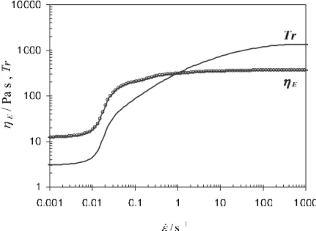
Collis et al.共2005兲, among others, have pointed out to the need of employing multi-mode multi-models in order to capture accurately the true relaxation response of actual polymer melts and solutions. Such recommendation has guided us in selecting the four-mode PTT constitutive model whose behavior has already been assessed in Sec. II for steady shear flow, by means of plots of the shear viscosity in Fig. 2 and the first normal stress difference coefficient in Fig. 3. However, the contraction flow also has important elon-gational flow regions and it is adequate at this stage to understand the behavior of the constitutive equation regarding its extensional viscosity. This is shown in Fig.4as a plot of both the steady extensional viscosity and the Trouton ratio versus the extensional rate of deformation in uniaxial extension. The behavior is typical of linear PTT models, with an increase in extensional viscosity to a plateau at high extensional rates, but the Trouton ratio keeps increasing to higher deformation rates because of the shear-thinning nature of the viscometric viscosity. For small values of␧ the plateaus of ␩E and Tr are inversely

proportional to this parameter.

C. Mesh characteristics

Although the sudden contraction geometry is symmetric relative to the two middle planes, all simulations were carried out on meshes covering the full wall-to-wall geom-etry in both directions, thus allowing for prediction of possible nonsymmetric flow pat-terns that might arise关as in the work ofPoole et al.共2007兲for a cross-slot geometry兴. As

a consequence, the only boundary conditions needed were no-slip at the solid walls and prescribed inlet and outlet boundary conditions. The inlet and outlet planes were

posi-tioned very far from the region of interest 共−100 H2 and 100 H2 for the Newtonian

simulations—meshes M40 and M80; −166.7 H2and 100 H2for the viscoelastic cases—

meshes M40U and M64兲, so that fully developed flow conditions were enforced. In the Newtonian calculations two meshes were used: mesh M40 had 40 cells in the upstream duct along each transverse direction, leading to a total of 51 000 computational cells. The refined mesh M80 had twice as many cells in each direction so it had a total number of 408 000 cells. The minimum normalized cell sizes 共⌬xmin/2H2=⌬ymin/2H2

=⌬zmin/2H2兲 were 0.05 for mesh M40 and 0.025 for mesh M80. For the viscoelastic

calculations two meshes were also used, one which had 40 uniform cells along each transverse direction 共on the upstream channel兲, with a total of 126 800 cells 共mesh M40U兲 and another mesh with 56 nonuniform cells in each transverse direction 共mesh M56兲, totaling 312 816 cells. The minimum normalized cell sizes were 0.10 for mesh M40U and 0.03 for mesh M56, respectively. Note that all these meshes, although coarser than those in the detailed 2D study ofAlves et al.共2003b兲, do represent a large increase in computational time because they correspond to 3D calculations leading to a significant increase in the number of degrees of freedom.

Local views of the four meshes in the contraction plane region are compared in Fig.5

where the nonuniform mesh structure is clearly visible. Preliminary simulations were initially carried out with both meshes, for each fluid type, to ascertain mesh convergence. The results obtained with both grids are similar共to within 3% accuracy, or better兲 but to obtain accurate results we decided to carry out all the ensuing simulations with the refined meshes for each case共mesh M80 for the Newtonian simulations and mesh M56 with the viscoelastic fluid兲, unless otherwise mentioned.

IV. RESULTS AND DISCUSSION

Comparison of experimental results from flow visualizations and numerical simula-tions are discussed first for Newtonian fluids and then for the viscoelastic fluid. Vis-coelasticity induces the inversion of the recirculation patterns in the corner vortices formed upstream of the contraction, in addition to enhanced vortices, eventually leading to flow instability.

FIG. 4. Steady-state extensional viscosity and Trouton ratio for the four-mode PTT plus Newtonian solvent

A. Newtonian fluid flow

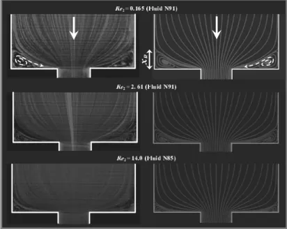
Flow visualizations in the 4:1 SQ/SQ contraction at different Reynolds numbers were carried out first with Newtonian fluids and here comparisons were also made with results of numerical simulations, as shown in Fig. 6. The Reynolds number is defined on the basis of the downstream duct, as

Re2=

␳U2共2H2兲

␩ . 共7兲

All flow visualizations in this work represent stream traces in the middle plane共z=0 or y = 0 planes兲 of the geometry. The numerical results shown on the right column of Fig.6

reproduce well the visualizations: under conditions of negligible inertia the normalized vortex size obtained in the middle plane is xR/2H1= 0.163共cf. Fig. 6 for xR definition兲,

but as inertia becomes non-negligible the size of the vortices decreases with Reynolds number and eventually the vortex vanishes at large flow rates. We note that due to symmetry the flow patterns are the same on the two middle planes y = 0 and z = 0. In Table

IIIwe present the predicted middle plane vortex sizes as function of the Reynolds num-ber. These data have benchmark quality, although for the two highest Reynolds number flows there is still some mesh dependency. Assuming that the numerical method has second-order accuracy关cf.Alves et al.共2003a;2003b兲兴, we can predict the extrapolated 共i.e., mesh independent兲 values of the vortex size, xR,ext. The estimated error between the

extrapolated values and the computed results on the refined mesh ranges from 0.1% for creeping flow, up to about 1.5% for the higher Reynolds number presented in TableIII. Even though the flow inside the vortices seen in Fig.6might look 2D, in reality it is highly 3D and none of the vortices are ever closed, in contrast with 2D flows. Under negligible inertia, the 3D flow pattern is rather complex and is illustrated in Fig.7. Let us consider two different symmetry planes in Fig.7: the middle共ABCD兲 plane

lar to the wall and always represented in the photos; the second共EFGH兲 plane at 45° to the wall and passing through opposite corners of the square cross section. In this second plane, henceforth referred to as corner共or diagonal兲 plane, no pictures could be taken but the descriptions below result from visual inspection of the flow as well as from the numerical calculations which were capable of capturing the observed flow features.

For the Newtonian fluids, the fluid particles entering the vortex at the corner plane, rotate towards its center and then drift along the eye of the 3D vortex towards the center of the middle-plane vortex. The particles at the middle-plane vortex rotate towards its periphery and exit the vortex at the reentrant corner flowing into the downstream duct, giving the impression that in this plane this vortex is closed. The experimental streak lines in the middle-plane vortex obtained by flow visualization, shown on the left side of Fig. 6, and the corresponding numerical streak lines, plotted on the right side, help understand the dynamics inside this vortex. In Fig. 7 we also present insets with the projected numerical streamlines on the middle and the diagonal planes, showing more clearly the different dynamics of the vortices on those two planes: while in the middle-plane vortex the flow is spinning outwards, and leaving through the small channel, inside the corner-plane vortex the opposite is happening, i.e., the fluid coming from upstream near the intersection of the walls共along line HF兲 is captured by the corner vortex.

FIG. 6. Experimental共left column兲 and numerical 共right column兲 streak lines for the flow of Newtonian fluids

N85 and N91 in the middle plane of a 4:1 SQ/SQ sudden contraction.

TABLE III. Influence of the Reynolds number on the vortex size in the

middle plane for Newtonian fluid flow.

Re2 0 0.165 2.61 14.0

xR/2H1共Mesh M40兲 0.1624 0.1597 0.1271 0.0756 xR/2H1共Mesh M80兲 0.1629 0.1602 0.1282 0.0792 xR,ext/2H1共Extrapolated兲 0.1631 0.1604 0.1286 0.0804

B. Viscoelastic fluid flow

The PAA500 fluid is shear thinning in viscosity, therefore the definition of Reynolds number is more ambiguous. Hence, the bulk velocity in the downstream duct is always indicated on the pictures. Note that the fluid has two limiting viscosities corresponding to the low and high shear-rate limits, which differ by a factor of 15 共cf. Fig. 2兲. In the

definition of the Reynolds number关cf. Eq.共7兲兴, we considered that the shear viscosity is evaluated at a characteristic shear rate of␥˙₂= U₂/H₂.

To quantify the elasticity a Deborah number is defined in terms of downstream flow conditions,

De₂=␭M共T兲U2

H₂ =

aT␭M共T0兲U2

H₂ , 共8兲

where␭Mrepresents Maxwell’s relaxation time which is calculated from the linear

vis-coelastic spectrum according to

␩p=

兺

兺

thus, for the PAA500 fluid the following values are obtained: ␩0=␩s+␩p= 4.07 Pa s, ␤

=␩s/␩0= 0.0663, and␭M= 20.5 s.

The influence of bulk velocity共or Deborah number兲, under conditions of low inertia, on the middle-plane vortex is illustrated by Fig. 8, which includes on the left column photos from the experimental visualizations, and on the right column streak lines from corresponding numerical simulations using the multimode PTT model. For this shear-thinning fluid intense vortex enhancement is seen, as in the experimental observations of

FIG. 7. Representative trajectories of fluid particles in the inertialess flow of a Newtonian fluid in the 3D 4:1

FIG. 8. Streak lines in the middle plane for the PAA500 fluid: experiments—left column; simulations—right

column. 共From top to bottom: U2= 0.226, 0.853, 3.33, 6.75 mm/s; De2= 1.54, 5.82, 22.7, 46.1; Re2

Evans and Walters共1986兲for the axisymmetric contraction. In fact, elastic shear-thinning fluids typically exhibit an intense corner vortex growth both in planar and axisymmetric contractions. The comparison between these visualizations and the numerical streak lines are remarkably similar up to U2= 6.75 mm/s 共De2= 46.1兲. For higher flow rates values of

xR are underpredicted, but further investigations are required here with different

vis-coelastic models that are able to better reproduce the rheological behavior of the PAA500 fluid, and more refined meshes. Nevertheless, we note that the calculations with mesh M56 are extremely expensive because of the very high relaxation time of the first mode: flow predictions at U2= 6.75 mm/s 共De2= 46.1兲 on this mesh took about 12 days of CPU

time in a personal computer based on the processor AMD Athlon XP 2400+ with 1 GHz of random access memory. Note that mesh M56 has 312 816 computational cells, corre-sponding to 8 758 848 degrees of freedom, a value considerably higher than any work documented so far in the computational rheology literature.

A second difference relative to the Newtonian flow is the shape of the vortices: whereas the middle-plane Newtonian vortex had a clear concave shape, for the shear-thinning fluid the vortex is neither concave nor convex at very low bulk velocities and becomes convex as the vortex grows with elasticity. The vortex length increases signifi-cantly with further increase in bulk velocity and at U2= 12.5 mm/s, corresponding to a

Deborah number of De2= 85.3, the vortex is very large as seen in Fig. 9, with xR/2H1

= 1.47. Further increase in the flow rate leads to a transition from the steady to a periodic unsteady flow and at U2= 16 mm/s the flow is already time dependent.

The vortex enhancement seen under steady flow conditions is much stronger for this shear-thinning fluid than was observed byAlves et al.共2005兲for Boger fluids. With view of elucidating the role of elasticity, Fig.10shows the influence of the Deborah number on the vortex size measured on the center plane 共xR/2H1兲. This figure also includes the

numerically predicted values of xR/2H1 for the PTT fluid, and the first point worth

noticing is a sudden reduction in the numerical rate of increase of vortex length with bulk velocity at high Deborah number flows. However, up to De2⬇40 the match between

numerical predictions and experimental measurements is remarkable, in line with the agreement also shown in the comparisons of Fig.8. We also include in Fig.10the vortex size on the corner plane 共x_R*/2H1—cf. Fig. 7 for definition兲 predicted numerically,

al-though for this plane no experimental data is available for comparison. Figure 10 also includes the predictions of xR/2H1 共and xR

*_/2H

1兲 for a generalized Newtonian fluid

共GNF兲, with a shear viscosity curve identical to that of the PAA500 fluid 共␩共GNF兲= 0.27

+ 3.80/关1+共20␥˙兲2_兴0.25_{, with ␩ and ␥˙ expressed in Pa s and s}−1_{, respectively兲. For this}

FIG. 9. Strong corner vortex enhancement for the flow of PAA500 fluid in the 3D 4:1 sudden contraction at U2= 12.5 mm/s 共De2= 85.3; Re2= 0.128兲.

inelastic fluid, the trend observed is not even qualitatively similar to the experimental data, thus demonstrating that the strong vortex enhancement observed is due to viscoelas-ticity, and more precisely as a result of the high extensional viscosity of the PAA500 fluid 共cf. Fig. 4兲. In order to substantiate this explanation, we have conducted additional

nu-merical simulations using different values of the ␧ parameter of the PTT model and keeping the remaining parameters unchanged. Due to the unavailability of rheometric data for the PAA500 fluid in extensional flow, there is some ambiguity on the adequate selection of the␧ parameter, which influences primarily the extensional viscosity and to a much lesser extent the shear viscosity共and ⌿1兲, as demonstrated in Fig.11. Therefore,

by varying this parameter we can assess how the extensional properties of the fluid influence the flow kinematics.

In Fig.12we plot the predicted vortex size as a function of De2for different␧ values,

illustrating that increasing the Trouton ratio 共or the extensional viscosity兲 leads to a significant increase of the vortex size. This plot also confirms that in order to accurately predict the experiments a small ␧ parameter should be selected, and the value ␧=0.02 indicated in Sec. II B for the multimode PTT model is appropriate. At the lower ␧ parameter simulated 共␧=0.01兲 numerical divergence was observed for De2= 46.1. The

rise in xR begins at De2⬇1, that is ␥˙2⬇0.05 s–1, which corresponds to a strain rate of

␧˙⬇共U2,c− U1,c兲/H1⬇2.1 U2共1−1/CR2兲/共CR H2兲⬇0.5 U2/H2⬇0.025 s−1 共note that for

a square channel the centerline velocity of a Newtonian fluid is nearly 2.1 times the average velocity in the channel: U2,c/U2= U1,c/U1⬇2.1兲. From Fig. 11 it is confirmed

that such value of␧˙ correlates well with the initial sharp increase in the Trouton ratio. It is therefore established that the inception of vortex enhancement follows from a sudden rise in the Trouton ratio vs. ␧˙ curve for a given fluid.

FIG. 10. Comparison between measured middle-plane vortex length in the SQ/SQ contraction for PAA500

fluid and predictions using a multimode PTT model. Also included are the predictions at the corner plane 共dashed lines兲 and predictions obtained with a GNF with a shear-viscosity curve identical to that of the PAA500 fluid. In this case the results were obtained for the same flow rate conditions as the viscoelastic fluid.

In Fig. 13we plot predicted profiles of pressure along the centerline共y=z=0兲, for a range of De2, for the parameters of the PAA500 fluid presented in Table II 共with ␰

= 0.04 and␧=0.02兲. In order to facilitate direct comparison between the different sets of data, we have normalized the pressure profiles as 共p−pref兲/共2␶w,2兲, where the reference

pressure, pref, was taken as the pressure at the location x/H2= −8. The characteristic wall

shear stress used in the normalization of the pressure profiles,␶w,2, refers to the average

value under fully developed flow conditions in the small channel, and can be related to the pressure gradient by 2␶w,2= H2共−dp/dx兲2,FD, where共dp/dx兲2,FDrepresents the

共con-FIG. 11. Shear viscosity␩共␥˙_{兲 and Trouton ratio Tr共␧˙兲 for the four-mode PTT plus Newtonian solvent model}

with different␧ values 共note that the shear viscosity used in the calculation of Tr is evaluated at␥˙ =冑3␧˙兲.

FIG. 12. Influence of the extensibility parameter␧ on the predictions of the middle-plane vortex size using the

multimode PTT model共mesh M40U兲, and comparison with measured data in the middle plane of the SQ/SQ contraction for PAA500 fluid. Also included are the predictions with a generalized Newtonian model with a shear-viscosity curve identical to that of the PAA500 fluid. In this case the results were obtained for the same flow rate conditions as the viscoelastic fluid.

stant兲 pressure gradient on the downstream channel under fully developed flow condi-tions. As shown in Fig.13, an increase of the flow rate共or De2兲 leads to a higher entrance

pressure drop, which can be quantified using a Couette correction coefficient, C, as plotted in the inset. The Couette correction is defined as a normalized entry 共or extra兲 pressure drop, C =共⌬p−⌬pFD兲/2␶w,2, where ⌬p represents the total pressure drop

be-tween one location far upstream of the contraction plane, and another point located far downstream of the entry region. The extra pressure drop is given by ⌬pext=⌬p−⌬pFD,

where ⌬pFD represents the pressure drop that would be observed between those two

locations if the flow was fully developed everywhere. The Couette correction is found to increase significantly with De₂, and there is a correlation with the increase of the Trouton ratio observed as␧˙ increases, as shown in Fig.11. In addition, in Fig.14共a兲we analyze the influence of␧ parameter on the pressure profiles along the centerline, for a relatively large and constant flow rate共U₂= 6.75 mm/s; De₂= 46.1兲. It is clear that a decrease of ␧ gives an enhancement of the entry pressure drop 共as better illustrated in the Couette correction plot shown as inset兲, thus being demonstrated that higher extensional viscosi-ties are directly related to larger flow resistance in the entrance region where extensional properties are all too important, as illustrated by the N1plots presented in Fig.14共b兲. We

note that even for the largest extensibility parameter tested共␧=0.8兲 the behavior although approaching that of an inelastic fluid with a similar shear viscosity curve still shows signs of slight vortex enhancement, thus giving further evidence of the importance of polymer extensibility upon the rise in entry pressure drop and on vortex enhancement. It is im-portant to emphasize here that although the shear viscosities are similar for the PTT model with a high␧ parameter 共which is viscoelastic兲 and for the generalized Newtonian model 共which is inelastic兲, in the latter there are no significant normal stresses in the extensional entry flow, while in the former those are not negligible as shown in Fig.

14共b兲, thus giving further credit to the importance of normal extensional stresses in the entry flow behavior.

Besides the enhanced corner vortex increase and the shape of the vortex, there is a third major difference between the viscoelastic and Newtonian fluid flow patterns: at high flow rates共or Deborah numbers兲 but still under conditions of steady flow, the direction of the secondary motion of fluid particles inside the vortices are inverted relative to those found at lower flow rates and with Newtonian fluids. This is clear from both the flow

FIG. 13. Pressure profiles along the centerline for different Deborah numbers De2predicted using the

visualizations and the numerical simulations, in particular those at higher flow rates in Fig.8. This new flow pattern is illustrated in the sketch of fluid particle trajectories in Fig.

15that corresponds to a bulk velocity of U2= 0.853 mm/s 共De2= 5.82兲. In contrast to the

observation for Newtonian fluids, the fluid coming from the upstream duct and entering the middle-plane vortex rotates towards its eye and then moves towards the eye of the corner-plane vortex where it rotates from the eye towards its periphery and exits the corner-plane vortex to the downstream duct. This flow pattern reversal is due to the effects of fluid elasticity and is well captured in the numerical simulations. The high extensional viscosity of the fluid is the most probable cause for this flow inversion since the effect is not captured by the simulations using the inelastic shear-thinning model under equivalent flow conditions. For all cases simulated numerically, we found that the flow inversion occurred when xR/2H1⬎0.22⫾0.02, thus indicating that vortex

enhance-FIG. 14. Influence of the ␧ parameter on the predicted 共a兲 pressure and 共b兲 N1 axial profiles along the

centerline, using the multimode PTT model共mesh M56兲 for U2= 6.75 mm/s 共De2= 46.1兲. Also included are the

predictions with a generalized Newtonian model with a shear-viscosity identical to that of the PAA500 fluid and a plot of the Couette correction vs␧ 关inset of 共a兲兴.

ment and flow inversion are related outcomes of fluid elasticity. For low values of ␧, vortex enhancement is stronger and flow reversal occurs at lower values of De2. For␧

= 0.8 flow reversal occurs for De2 between 22.7 and 46.1, while for␧=0.02 flow

inver-sion is already observed at De2= 5.82.

As already mentioned, at high flow rates the flow of PAA500 becomes unsteady but periodic, in the same way as previously observed for Boger fluids byAlves et al.共2005兲

in the same geometry. For an upstream bulk velocity of U2= 18.2 mm/s, which

corre-sponds to De2= 124 and Re2= 0.208, the sequence of photographs presented in Fig. 16

represents three different moments within a cycle of flow periodicity. Obviously, the periodicity is happening in both transverse directions. From films taken with a movie camera at a known frame rate it was possible to estimate the frequency共f兲 of oscillation for different flow rates within the periodic regime. This frequency varied linearly with flow rate defining a constant Strouhal number St= 2fH1/U1⬇0.5.

We speculate that at higher flow rates, not attained in these experiments, further elastic instabilities will grow and turn the flow chaotic. Predictions of the observed flow features will require a full 3D, time-dependent simulation of the whole geometry with an adequate constitutive model, a challenge to be undertaken in the future.

V. CONCLUSIONS

Flow visualizations and numerical simulations were carried out in a 4:1 sudden SQ/SQ contraction for Newtonian and viscoelastic shear-thinning fluids under conditions of low

FIG. 15. Representative trajectories of fluid particles in the inertialess flow of PAA500 in the 3D 4:1 sudden

contraction flow共U2= 0.853 mm/s, De2= 5.82, Re2= 0.0032兲. The projected stream traces on the middle and

inertia. For the 3D numerical simulations a finite-volume code was used and a four-mode linear PTT plus Newtonian solvent model simulated the rheology of the non-Newtonian fluid.

For the Newtonian fluid the numerical flow patterns in the middle plane are in excel-lent agreement with experimental results. The flow field is clearly 3D with fluid particles moving from the upstream duct and entering the corner-plane vortex, rotating towards its center, and then drifting to the eye of the middle-plane vortex where they rotate to the outside of the vortex and exit at the reentrant corner into the downstream duct. For the non-Newtonian fluid the visualizations reveal that very significant changes in fluid dy-namics are taking place under inertialess flow conditions: the vortices became convex in shape and grew significantly in size due to fluid elasticity, and the vortices and the dynamics of the secondary flow at high flow rates have been reversed with fluid particles entering the middle-plane vortex and exiting at the corner-plane vortex. At even higher flow rates the long vortices became unstable and a periodic flow emerged. The numerical simulations predicted well the measured flow patterns at low flow rates provided the extensibility parameter of the PTT model was properly chosen, but underpredicted the vortex length at higher flow rates near the critical conditions that lead to the onset of an elastic instability. No simulations were attempted under these critical conditions where unsteady flow is observed. It was demonstrated that the elongational properties of the fluid are a key quantity in determining correctly both the size of the vortices formed upstream of the contraction and the entry pressure drop.

FIG. 16. Instantaneous flow patterns for a supercritical flow rate for fluid PAA500 共U2= 18.2 mm/s, De2

ACKNOWLEDGMENTS

M.A.A. acknowledges funding by Fundação para a Ciência e a Tecnologia共Portugal兲 and FEDER through program POCI 2010共project POCI/EQU/59256/2004兲.

References

Alves, M. A., P. J. Oliveira, and F. T. Pinho, “A convergent and universally bounded interpolation scheme for the treatment of advection,” Int. J. Numer. Methods Fluids 41, 47–75共2003a兲.

Alves, M. A., P. J. Oliveira, and F. T. Pinho, “Benchmark solutions for the flow of Oldroyd-B and PTT fluids in planar contractions,” J. Non-Newtonian Fluid Mech. 110, 45–75共2003b兲.

Alves, M. A., D. Torres, M. P. Gonçalves, P. J. Oliveira, and F. T. Pinho, “Visualization studies of viscoelastic flow in a 4:1 square/square contraction,” COBEM 2003, 17th International Congress of Mechanical Engi-neering, São Paulo, Brazil 2003, 2003c.

Alves, M. A., P. J. Oliveira, and F. T. Pinho, “On the effect of contraction ratio in viscoelastic flow through abrupt contractions,” J. Non-Newtonian Fluid Mech. 122, 117–130共2004兲.

Alves, M. A., F. T. Pinho, and P. J. Oliveira, “Visualizations of Boger fluid flows in a 4:1 square-square contraction,” AIChE J. 51, 2908–2922共2005兲.

Alves, M. A., and R. J. Poole, “Divergent flow in contractions,” J. Non-Newtonian Fluid Mech. 144, 140–148 共2007兲.

Boger, D. V., “Viscoelastic flows through contractions,” Annu. Rev. Fluid Mech. 19, 157–182共1987兲. Boger, D. V., and K. Walters, Rheological Phenomena in Focus共Elsevier, Amsterdam, 1993兲.

Boger, D. V., D. U. Hur, and R. J. Binnington, “Further observations of elastic effects in tubular entry flows,” J. Non-Newtonian Fluid Mech. 20, 31–49共1986兲.

Brown, R. A., and G. H. McKinley, “Report on the VIIIth International Workshop on Numerical-Methods in Viscoelastic Flows,” J. Non-Newtonian Fluid Mech. 52, 407–413共1994兲.

Cable, P. J., and D. V. Boger, “A comprehensive experimental investigation of tubular entry flow of viscoelastic fluids: Part I. Vortex characteristics in stable flow,” AIChE J. 24, 868–879共1978a兲.

Cable, P. J., and D. V. Boger, “A comprehensive experimental investigation of tubular entry flow of viscoelastic fluids: Part II. The velocity fields in stable flow,” AIChE J. 24, 992–999共1978b兲.

Cable, P. J., and D. V. Boger, “A comprehensive experimental investigation of tubular entry flow of viscoelastic fluids: Part III. Unstable flow,” AIChE J. 25, 152–159共1979兲.

Carvalho, J. R. F. G., J. M. P. Q. Delgado, and M. A. Alves, “Diffusion cloud around and downstream of active sphere immersed in granular bed through which fluid flows,” Chem. Eng. Sci. 62, 2813–2820共2007兲. Coates, P. J., R. C. Armstrong, and R. A. Brown, “Calculation of steady-state viscoelastic flow through

axi-symmetrical contractions with the EEME formulation,” J. Non-Newtonian Fluid Mech. 42, 141–188 共1992兲.

Collis, M. W., A. K. Lee, M. R. Mackley, R. S. Graham, D. J. Groves, A. E. Likhtman, T. M. Nicholson, O. G. Harlen, T. C. B. McLeish, L. R. Hutchings, C. M. Fernyhough, and R. N. Young, “Constriction flows of monodisperse linear entangled polymers: Multiscale modeling and flow visualization,” J. Rheol. 49, 501– 522共2005兲.

Crochet, M. J., A. R. Davies, and K. Walters, Numerical Simulation of Non-Newtonian Flow共Elsevier, New York, 1984兲.

Evans, R. E., and K. Walters, “Flow characteristics associated with abrupt changes in geometry in the case of highly elastic liquids,” J. Non-Newtonian Fluid Mech. 20, 11–29共1986兲.

Evans, R. E., and K. Walters, “Further remarks on the lip-vortex mechanism of vortex enhancement in planar contraction flows,” J. Non-Newtonian Fluid Mech. 32, 95–105共1988兲.

Ferreira, V. G., C. M. Oishi, F. A. Kurokawa, M. K. Kaibara, J. A. Cuminato, A. Castelo, N. Mangiavacchi, M. F. Tomé, and S. McKee, “A combination of implicit and adaptative upwind tools for the numerical solution of incompressible free surface flows,” Commun. Numer. Methods Eng. 23, 419–445共2007兲.

Hassager, O., “Working group on numerical techniques. Fifth International Workshop on Numerical Methods in Non-Newtonian Flows, Lake Arrowhead, USA,” J. Non-Newtonian Fluid Mech. 29, 2–5共1988兲. Khosla, P. K., and S. G. Rubin, “A diagonally dominant second-order accurate implicit scheme,” Comput.

Fluids 2, 207–209共1974兲.

Lee, K., M. R. Mackley, T. C. B. McLeish, T. M. Nicholson, and O. G. Harlen, “Experimental observation and numerical simulation of transient stress fangs within flowing molten polyethylene,” J. Rheol. 45, 1261– 1277共2001兲.

McKinley, G. H., W. P. Raiford, R. A. Brown, and R. C. Armstrong, “Nonlinear dynamics of viscoelastic flow in axisymmetric abrupt contractions,” J. Fluid Mech. 223, 411–456共1991兲.

Mompean, G., and M. Deville, “Unsteady finite volume simulation of Oldroyd-B fluid through a three-dimensional planar contraction,” J. Non-Newtonian Fluid Mech. 72, 253–279共1997兲.

Oliveira, P. J., and F. T. Pinho, “Numerical procedure for the computation of fluid flow with arbitrary stress-strain relationships,” Numer. Heat Transfer, Part B 35, 295–315共1999兲.

Oliveira, P. J., F. T. Pinho, and G. A. Pinto, “Numerical simulation of non-linear elastic flows with a general collocated finite-volume method,” J. Non-Newtonian Fluid Mech. 79, 1–43共1998兲.

Oliveira, M. S. N., F. T. Pinho, P. J. Oliveira, and M. A. Alves, “Effect of contraction ratio upon viscoelastic flow in contractions: The axisymmetric case,” J. Non-Newtonian Fluid Mech. 147, 92–108共2007兲. Owens, R. G., and T. N. Phillips, Computational Rheology共Imperial College Press, London, 2002兲. Phan-Thien, N., and R. I. Tanner, “A new constitutive equation derived from network theory,” J.

Non-Newtonian Fluid Mech. 2, 353–365共1977兲.

Poole, R. J., M. A. Alves, and P. J. Oliveira, “Purely-elastic flow asymmetries,” Phys. Rev. Lett. 99, 164503 共2007兲.

Purnode, B., and M. J. Crochet, “Flows of polymer solutions through contractions. Part 1: Flows of polyacry-lamide solutions through planar contractions,” J. Non-Newtonian Fluid Mech. 65, 269–289共1996兲. Quinzani, L. M., R. C. Armstrong, and R. A. Brown, “Birefringence and laser-Doppler velocimetry 共LDV兲

studies of viscoelastic flow through a planar contraction,” J. Non-Newtonian Fluid Mech. 52, 1–36共1994兲. Rothstein, J. P., and G. H. McKinley, “Extensional flow of a polystyrene Boger fluid through a 4:1:4

axisym-metric contraction/expansion,” J. Non-Newtonian Fluid Mech. 86, 61–88共1999兲.

Santos, J. C., P. Cruz, M. A. Alves, P. J. Oliveira, F. D. Magalhães, and A. Mendes, “Adaptive multiresolution approach for two-dimensional PDEs,” Comput. Methods Appl. Mech. Eng. 193, 405–425共2004兲. Sirakov, I., A. Ainser, M. Haouche, and J. Guillet, “Three-dimensional numerical simulation of viscoelastic

contraction flows using the Pom–Pom differential constitutive model,” J. Non-Newtonian Fluid Mech. 126, 163–173共2005兲.

Walters, K., and D. M. Rawlinson, “On some contraction flows for Boger fluids,” Rheol. Acta 21, 547–552 共1982兲.

Walters, K., and M. F. Webster, “On dominating elastico-viscous response in some complex flows,” Philos. Trans. R. Soc. London, Ser. A 308, 199–218共1982兲.

Walters, K., and M. F. Webster, “The distinctive CFD challenges of computational rheology,” Int. J. Numer. Methods Fluids 43, 577–596共2003兲.

Xue, S. C., N. Phan-Thien, and R. I. Tanner, “Three dimensional numerical simulations of viscoelastic flows through planar contractions,” J. Non-Newtonian Fluid Mech. 74, 195–245共1998a兲.

Xue, S. C., N. Phan-Thien, and R. I. Tanner, “Numerical investigations of Lagrangian unsteady extensional flows of viscoelastic fluids in 3-D rectangular ducts with sudden contractions,” Rheol. Acta 37, 158–169 共1998b兲.