INVESTMENT AND EXCLUSIVE AGREEMENTS
LUÍS VASCONCELOSy
Abstract. I analyze a simple model of hold-up with asymmetric information at the con-tracting stage. I show that contractual signalling and e¢ ciency of investment can con‡ict if only quantity is contractible. This is because contracted quantity encourages investment in the relationship but also signals information. This con‡ict generates ine¢ cient equilib-ria in terms of investment. Contracting on exclusivity in addition to quantity resolves the con‡ict (and consequently eliminates the ine¢ ciency of investment) when the asymmetry of information concerns the value of trade with external parties. While exclusivity also signals information, unlike quantity it does not directly a¤ect relationship-speci…c investment.
Keywords: Relationship-speci…c investment, asymmetric information, hold-up, exclusiv-ity.
JEL Classi…cation: L14, L40, D82, K21
1. Introduction
Many relationships are formed under asymmetric information. When two or more parties meet to agree on the terms of a future relationship, some of them may have relevant private information about how successful the relationship will be. For example, in vertical relation-ships, a …nal good producer contracting with a speci…c supplier about future trade may have private information about her future value of trading with the supplier. Similarly, a manufac-turer o¤ering a franchising agreement to a retailer may be better informed than the retailer about the retailer’s ability to sell his product. As was emphasized by Myerson (1983) and Maskin and Tirole (1992), in these cases, if the parties with private information participate in the design of the contract (or the terms of the relationship if established in an informal way), the contract’s terms may reveal some of their private information to the other parties. Because of this information transmission e¤ect, the design of the contract assumes a strategic role not present when contracting parties have symmetric information. If investment in the
Date: December 2007.
I especially thank Mike Whinston, for extremely valuable suggestions. I also thank Adeline Delavande, Alessandro Pavan, Allan Collard-Wexler, Asher Wolinsky, Bentley MacLeod, Fabio Braggion, Juan Carrillo, Ran Abramitzky, William Rogerson, and seminar participants at Columbia University, Northwestern Univer-sity, University of Rochester, Universidade Nova de Lisboa, and University of Southern California. Financial support from the Fundação para a Ciência e Tecnologia and the Northwestern University Center for the Study of Industrial Organization are gratefully acknowledged.
yContact information: L-vasconcelos@fe.unl.pt. Universidade Nova de Lisboa, Faculdade de Economia,
Cam-pus de Campolide, 1099-032 Lisboa, Portugal.
relationship is important, this role is in addition to the e¢ ciency role of providing the parties with the right incentives to invest that is typical to the hold-up problem literature.
In this paper, I consider a simple model of hold-up with asymmetric information at the contracting stage. In the model a principal (e.g., a buyer) with private information wishes to encourage an agent (e.g., a supplier) to make a relationship-speci…c investment. I analyze how the two roles of contracting mentioned above interact with one another and highlight a pro-e¢ ciency role of exclusivity agreements. I …rst consider the case of quantity contracts (or, so-called speci…c-performance contracts, which specify the default number of units the parties will trade) and show that because of information concerns, the principal may distort the contract’s terms away from those that generate incentives for e¢ cient investment in the relationship. I then consider the case of contracts that in addition to quantity specify an exclusivity clause that restricts the principal to trade only with the agent, and show that exclusivity plays an important role in eliminating such contractual distortions and thereby the ine¢ ciency of investment. This result rationalizes the use of contracts that specify both quantity and exclusivity. It also rationalizes the use of exclusivity in situations of hold-up with pure relationship-speci…c investments.
Both the contractual distortions and the e¤ect of contractibility of exclusivity on relationship-speci…c investment highlighted here are novel in the literature. This is because the existing literature on the hold-up problem (e.g., Grossman and Hart, 1986; Edlin and Reichelstein, 1996; and Che and Hausch, 1999), and in particular that on the interaction between exclu-sivity and relationship-speci…c investment (e.g., Segal and Whinston, 2000; and De Meza and Selvaggi, 2007), has focused on situations where parties’information is symmetric at the initial contracting stage.
The model I consider is a standard model of hold-up, with the exception that at the con-tracting stage the party who proposes the contract has private information. Speci…cally, I consider a model in which a principal and an agent …rst meet and contract about future transactions, while knowing that later on, the principal may wish to trade with an external party instead. Possible contractual agreements include: a contracted quantity, which corre-sponds to the default quantity that parties will trade; and a contracted level of exclusivity, restricting the principal to trade only with the agent. At the initial contracting stage, both parties are uncertain about the value of the relationship, but the principal has better infor-mation about how successful it will be. This is either because she is better informed about how much she values trade with the agent (private internal information) or because she is better informed about the value of her future outside options (private external information). I consider both cases of internal and external information because, as I show, the source of asymmetry of information a¤ects which forms of contractual commitment are e¤ective in signalling information. Once both parties agree on a contract, a relationship is formed and the agent has the opportunity to invest in it. At a latter date, uncertainty is realized and both the principal and the agent observe the value of trading with each other and the value of the principal’s trade with others. At this point, the principal and agent renegotiate the
initial contract whenever it is ine¢ cient.1 Although renegotiated, the initial contract still
matters because it determines the status quo positions of both parties (disagreement point) during renegotiation.
I …nd that if the contract can specify quantity but not exclusivity, signalling information by the principal to extract surplus from the agent and e¢ ciency of investment can con‡ict with one another. This con‡ict generates ine¢ cient equilibria, as the principal contracts a quantity that distorts the agent’s investment decision relative to its socially e¢ cient level to signal information. I also show that when the principal’s private information is internal, con-tractibility of exclusivity does not a¤ect the set of equilibrium outcomes. As a consequence, when the principal has private internal information only, the possibility to use exclusivity in addition to quantity in the contract does not play any role in mitigating the con‡ict between surplus extraction and investment incentives.
I …nally show that in contrast with the case of internal information, when the principal’s private information is external, the con‡ict between signalling information to extract surplus and investment incentives can be resolved if the principal can use both quantity and exclu-sivity in the contract. This is because, when the principal’s private information is about the value of her outside option, exclusivity serves as a strong signal of that information; and because, in contrast to contracted quantity, exclusivity does not a¤ect directly the agent’s investment decision. Thus, when both quantity and exclusivity are contractible, the princi-pal can set contracted quantity to induce optimal investment by the agent, and then adjust contracted exclusivity, without a¤ecting the agent’s investment decision, in a way that the combination of the signalling e¤ects of contracted quantity and exclusivity allow her to signal information and extract surplus.
The e¢ ciency e¤ect of exclusivity identi…ed here is important for two reasons. First, in con-trast to Segal and Whinston (2000), it rationalizes the use of exclusive contracts in situations of hold-up with pure relationship-speci…c investments. Motivated by informal discussions (in anti-trust and exclusive contracts) on whether exclusive provisions foster relationship-speci…c investments, Segal and Whinston (2000) show that exclusivity does not a¤ect whatsoever in-vestments that are fully relationship-speci…c, when information is symmetric at the contract-ing stage.2 Second, it contributes to the unsettled debate on whether exclusive agreements
1By considering that parties observe valuations of trade and subsequently renegotiate the initial contract,
two important features of many relationships are captured. First, parties to a relationship often learn its real value (only) after the relationship has started. Second, in those cases, parties tend to renegotiate initial contracts that are ine¢ cient ex-post. Beaudry and Poitevin (1993) study equilibrium contracting by an informed party in a setting with renegotiation. They consider the case in which the asymmetry of information persists during the renegotiation stage.
2In De Meza and Selvaggi (2007), the authors show that exclusivity may a¤ect relationship-speci…c
in-vestments. Their result di¤ers from that in Segal and Whinston (2000) because they consider a di¤erent bargaining game. Our e¤ect is totally di¤erent from that in De Meza and Selvaggi (2007), as it stems from the existence of asymmetric information at the contracting stage.
should be contractually allowed by courts or not. In this speci…c matter, a long-standing con-cern of courts is that exclusive contracts serve anticompetitive purposes, and consequently prevent e¢ ciency.
By studying contractual signalling by an informed party in the presence of relationship-speci…c investment, this paper is inherently related to two strands of the literature: the literature on the hold-up problem and the literature on contract design by an informed party. The existing literature on the hold-up problem assumes symmetric information at the initial contracting stage (e.g., Hart and Moore, 1990; Chung, 1991; Rogerson, 1992; MacLeod and Malcomson, 1993; Aghion et al., 1994; and Segal and Whinston, 2000). By studying contract design by an informed party in a relationship with speci…c investments, this paper extends the literature on the hold-up problem to the case in which there is asymmetric information at the contracting stage. In the hold-up problem literature (with symmetric information at the contracting stage), the contract is typically designed with one goal: to provide the right incentives to invest. The presence of asymmetric information at the contracting stage introduces a new role for the contract: signalling information to extract surplus.
The literature on contract design by an informed principal can be divided into two groups. The …rst group focuses on the characterization (in a general way) of the equilibrium contract proposal by an informed principal in a principal-agent relationship (e.g., Myerson, 1983; Maskin and Tirole, 1990; Maskin and Tirole, 1992; and Beaudry and Poitevin, 1993). The modelling approach is this paper is in the spirit of that in Maskin and Tirole (1992). In the context of the model in this paper, I extend their analysis and results to the case in which the agent makes a noncontractible investment decision. This extension is not a trivial one. Maskin and Tirole (1992) assume that all payo¤ relevant variables are contractible. In their model, the agent’s beliefs about the principal’s type a¤ect only the agent’s decision to accept the contracts proposed by the principal. In the model in this paper those beliefs also a¤ect the agent’s investment decision, which in turn a¤ects the principal’s payo¤ (and preferences over contracts). So, in here, the agent’s beliefs at the end of the contracting phase are still important. The second group of this literature has studied contract design by an informed party in more concrete settings (e.g., Aghion and Bolton, 1987; Aghion and Hermalin, 1990; Spier, 1992; and Nosal, 2006).3 The articles in this literature have not studied speci…cally
the relationship between contractual signalling and relationship-speci…c investment.
The paper is structured as follows. In Section 2, I present the model. In Section 3, I establish the result that exclusivity is irrelevant in terms of equilibrium outcomes when the principal’s private information is internal. In Section 4, I analyze equilibrium outcomes when contracts specify only quantity and then when contracts can specify both quantity
3For example, Aghion and Hermalin (1990) use a contract signalling model to show that imposing
le-gal restrictions on private contracts can enhance e¢ ciency. Spier (1992) identi…es a reason for contractual incompleteness by showing that an informed principal can signal information by deliberately proposing an incomplete contract to an agent. Nosal (2006) considers a situation of contract signalling when studying the incentives of a principal to acquire private information before contracting with an agent.
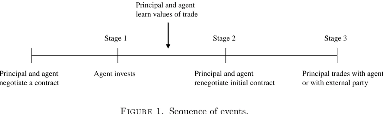
Principal and agent negotiate a contract
Agent invests
Principal and agent learn values of trade
Principal and agent renegotiate initial contract
Principal trades with agent or with external party
Stage 1 Stage 2 Stage 3
Figure 1. Sequence of events.
and exclusivity. I show the existence of ine¢ cient equilibria in terms of investment and how exclusivity resolves this ine¢ ciency. In Section 5, I present concluding remarks.
2. The Model
The model delineated in this section and the subsequent analysis are presented in terms of a generic trade relationship between a principal with private information and an agent who can invest in the relationship by preparing for trade. The following are trivial applications of the model: (i) a buyer with private information about how much she values a given product contracting with a supplier about the quantity to be delivered, when the supplier still has to design the product and initiate its production; (ii) a manufacturer with private information about her production cost contracting with a retailer about supply conditions (e.g., quantity and/or the concession of an exclusive territory to the retailer), when the retailer still has to invest in the handling, proper storage and promotion of the manufacturer’s product. I next present the model.
Players and sequence of events. Consider a principal and an agent who initially contract, knowing that the principal may later wish to deal with an external party instead. If they agree on a contract, a relationship is formed. If not, the principal and agent obtain their reservation payo¤s (which are the expected value of dealing later with an external party and zero, respectively) and the game ends.
Once a relationship is formed, it evolves in three stages: (i) an investment stage, in which the agent has the opportunity to make a relationship-speci…c investment a 2 A R+0;
(ii) a renegotiation stage, which occurs after uncertainty about trade valuations is realized and where the principal and the agent renegotiate the terms of the initial contract; and (iii) a trading stage. Trade between the principal and the agent may never occur. At the renegotiation stage, parties may decide not to deal with each other if after uncertainty is resolved it is actually more e¢ cient for the principal to trade with an external party than with the agent. The sequence of events is illustrated in Figure 1.
Payoffs. The parties’payo¤s are quasi-linear in money. The agent’s payo¤ is additive in the investment cost, which is denoted by (a) and assumed to be increasing in a. In addition to any money transfers, if at the trading stage the principal and agent trade with each other,
they obtain values of vP and vA, respectively. For future convenience, the value of trade
between the principal and the agent is denoted V vP + vA.4 The value of trade between
the principal and an external party is denoted by VE. For simplicity, I assume that VE is
always non-negative.
Information. During the contracting and investment stages (ex-ante) trade valuations are still uncertain, but the principal is better informed about them than the agent. This is formalized by assuming that the principal knows the true state of the world 2 f L; Hg,
while the agent knows only its prior probability p( ); and by assuming that the joint distri-bution of the valuations vP, vA and VE depends not only on the agent’s investment a but
also on state , i.e., (vP; vA; VE) F (: j a; ). After the investment stage, but before
rene-gotiation, uncertainty is realized and both the principal and agent observe the realization of valuations vA, vP and VE. Hence, renegotiation and trading (ex-post ) occur under symmetric
information. Although observable by the parties, valuations cannot be veri…ed by a court. Therefore, contracts that are directly contingent on valuations are not feasible.
Contracting. At the contracting stage, the principal has the opportunity to make a “take it or leave it” o¤er to the agent of a …nite menu of contracts. If the agent accepts the menu, the principal herself then chooses a contract from the menu (throughout, the principal is feminine and the agent is masculine). This is the contract that governs the relationship between the principal and the agent. By allowing the principal to propose menus of contracts, I follow an approach similar to that in Maskin and Tirole (1992) when analyzing the problem of mechanism design by an informed principal.
The potentially contractible variables are: an up-front transfer t from the agent to the principal, a quantity q, and a level of exclusivity e. The up-front transfer can take any real value, t 2 R. (A negative t corresponds to a transfer from the principal to the agent.) Quan-tity q denotes the probability that the principal and the agent must trade. The exclusivity variable e denotes the probability that the agreement is exclusive; i.e., that the principal cannot trade with an external party.5 Throughout, the set of allowable quantities is denoted by Q and that of allowable exclusivity levels by E. When both quantity and exclusivity are contractible, Q = [0; 1] and E = [0; 1]. Noncontractible exclusivity is modeled by imposing E = f0g. A contract is an object of the form c = (t; q; e) 2 C, where C = R Q E. The agent’s investment decision is not veri…able and therefore cannot be contractually speci…ed.6
4Suppose, for example, that the principal is a buyer, the agent is seller with production cost c, and the buyer needs at most one unit of the seller’s product. In this case, vP corresponds to the buyer’s valuation of
the seller’s product and vA= c. The value created if the buyer and the seller trade is V = vP+ vA= vP c.
5The quantity and exclusivity variables can be interpreted as proportions of trade capacity. Under this interpretation, quantity q represents the proportion of the trade capacity of the principal that is contractually allocated to the agent, and exclusivity e represents the proportion of the remaining (1 q) of the trade capacity of the principal that cannot be traded with an external party. The assumption that e is a proportion is not crucial. All the results in the paper hold if contracts can only prescribe full exclusivity (e = 1) or full non-exclusivity (e = 0).
6The existence of relationship-speci…c investments that are noncontractible has been the fundamental as-sumption in the hold-up problem literature. Relationship-speci…c investments often take a nonmonetary,
Renegotiation. After observing the realization of the valuations, if the initial contract prescribes an ine¢ cient level of trade, the principal and the agent renegotiate trade to the e¢ cient level. The agent’s investment decision is irreversible at this stage. As in Edlin and Reichelstein (1996), Che and Hausch (1999), Segal and Whinston (2000) and Segal and Whinston (2002), I assume that the bargaining shares of the principal and the agent during renegotiation are exogenously speci…ed. More speci…cally, I assume that the principal and the agent equally divide their renegotiation surplus over the disagreement point, which is determined by the original contract.7 Thus, despite renegotiation, the original contract still matters because it a¤ects the distribution of ex-post surplus, which in turn is important for surplus extraction by the principal and investment by the agent. Finally, I suppose that the external party with whom the principal can alternatively deal receives no surplus. This would be consistent, for instance, with a case of competition among many external parties who are willing to deal with the principal in the event she does not trade with the agent.
An implicit assumption in the model is that the agent gains some bargaining power during the relationship. This corresponds to situations where by investing in preparation for trade or by direct contact with the principal, the agent learns more about the principal (e.g., about technology employed, …nancial position, negotiation strategies) leaving him in a better position in future negotiations.
In the analysis that follows, the equilibrium concept used is the Perfect Bayesian Equilib-rium (PBE).8
2.1. Post-Renegotiation Payo¤s, Expected Payo¤s and Agent’s Investment. At the renegotiation stage, the principal and agent receive one half of the renegotiation surplus in addition to their disagreement payo¤s. The disagreement payo¤s of the principal and agent are the payo¤s in the event they do not reach a renegotiation agreement and the initial contract is executed. The renegotiation surplus is the di¤erence between the e¢ cient total surplus and the sum of the disagreement payo¤s. Since the disagreement payo¤s (ignoring sunk investment costs) are qvA t for the agent and qvP + (1 q)(1 e)VE + t for the
principal, and the e¢ cient total surplus (also ignoring sunk investment costs) is maxfV; VEg,
the agent’s post-renegotiation payo¤ given contract c = (t; q; e) and (a; vA; vP; VE) is
intangible form, such as human capital investment. In these cases, it is di¢ cult to contract on investment-related information.
7The assumption that the principal and the agent have equal bargaining shares at the renegotiation stage is not crucial. All the results remain unchanged if instead of 1/2 we consider that the agent’s bargaining share is 2 (0; 1). The important assumption is that the agent has some (strictly positive) bargaining power at the renegotiation stage. Otherwise, his payo¤ would not depend on the private information of the principal, in which case there is no need for the principal to signal her private information to be able to extract surplus from the agent.
given by
uA(c; ) = (qvA t) +
1
2[maxfV; VEg (qvA t) (qvP + (1 q)(1 e)VE+ t)] (a)
= 1
2maxfV; VEg 1
2[q(vP vA) + (1 q)(1 e)VE] t (a). (1)
Similarly, the principal’s post-renegotiation payo¤ can be written as (2) uP(c; ) =
1
2maxfV; VEg + 1
2[q(vP vA) + (1 q)(1 e)VE] + t.
E¢ cient renegotiation implies that the sum of the payo¤s to principal and agent is always equal to e¢ cient total surplus (hereinafter, total surplus), i.e., uA(c; ) + uP(c; ) = s( ), for
all c and , where s( ) = maxfV; VEg (a).
Since the analysis will focus on the equilibrium of the contracting game between the princi-pal and the agent, which occurs before uncertainty is resolved, it is convenient to obtain their ex-ante expected payo¤s. The expected payo¤s of the principal and agent are both functions of the contract c and the agent’s investment level a. However, since at the contracting and investment stages the principal knows and the agent does not, the expected payo¤ of the principal is a direct function of , while the expected payo¤ of the agent is a function of his beliefs about . More speci…cally, expected payo¤s are given by
UA(c; a j bH) = (1 bH)E[uAj a; L] + bHE[uAj a; H]
and
UP(c; a j ) = E[uP j a; ], all 2 ,
where bH 2 [0; 1] represents the agent’s belief that = H. With a slight abuse of notation,
UA(c; a j 0) and UA(c; a j 1) will be frequently denoted by UA(c; a j L) and UA(c; a j H),
respectively.
The expected total surplus given investment a and state is denoted by S(a; ) E[s( ) j a; ]. From the fact that uA(c; ) + uP(c; ) = s( ) for all c and , it follows that for any
2 and a 2 A,
(3) UA(c; a j ) + UP(c; a j ) = S(a; ) for all c 2 C.
This property of the expected payo¤s will be extensively used in the analysis of the equilibrium outcomes.
The …rst-best level of investment given state j, denoted by a0j, is the investment that
maximizes total expected surplus, i.e.,
a0j arg max
a2A
S(a; j).
The agent’s investment decision, denoted by a (c; bH), is the investment level that maximizes
his expected payo¤ given contract c and beliefs bH, i.e.,
(4) a (c; bH) arg max
a2A
It is assumed that S(a; ) and UA(c; a j ) are concave in a for all 2 , and that both
a0j and a (c; bH) are interior to A. It is also assumed that S(a; ) is di¤erentiable in a and
UA(c; a j ) is twice continuously di¤erentiable in a for all 2 .9
3. Internal Information and Exclusives: An Irrelevance Result
I begin the analysis by showing that when the principal has no private information about her value of trade with the external parties VE, then contracting on exclusivity does not
expand the set of equilibrium outcomes. More speci…cally, I show that for any equilibrium when the contract space is C = R Q E, there is an equilibrium with identical expected payo¤s and identical agent investment when the contract space is C0 = R Q f0g. For
future reference, equilibria satisfying this property are called outcome equivalent.
This result is established here for expositional convenience. Speci…cally, because it will be useful in the next section and because it holds regardless of the way in which the agent’s investment a and the state a¤ect the distribution of internal values vA and vP— e¤ects
about which I will be more speci…c further on. Hereinafter, let FVE(: j ) denote the marginal
cumulative distribution function of VE given state .10
Proposition 1 (Irrelevance Result). Suppose that the principal’s private information does not include information about the principal’s value of trade with external parties, i.e., FVE(: j
) = FVE(:) for all 2 . Then, exclusivity has no e¤ect on the set of equilibrium outcomes:
for any equilibrium when the contract space is C = R Q E, there is an outcome equivalent equilibrium when the contract space is C0 = R Q f0g:
Proof. See Appendix B.
There are two crucial points in understanding this result. First, since investment a¤ects internal values only, there is no cross e¤ect between investment and exclusivity in the payo¤ functions. This implies that exclusivity has no direct e¤ect on the agent’s investment decision. Second, since information is only about internal values, there is also no cross e¤ect between exclusivity and private information in the expected payo¤ functions of the principal and the agent. In other words, the expected payo¤s of the principal and the agent do not satisfy the single crossing property with respect to exclusivity. Thus, for given beliefs, the principal can exchange exclusivity by up-front transfer in the contract and still generate the same expected payo¤s and the same agent’s investment decision.
The irrelevance result in this section extends that in Segal and Whinston (2000) to a setting with asymmetric information. In that paper, the authors show that exclusivity has no e¤ect on investment decisions when investment a¤ects only internal values. Proposition 1 implies
9Concavity of S(a; ) and U
A(c; a j ) in a ensures that a (c; bH)and a0j are unique. Di¤erentiability of
S(a; )and UA(c; a j ) in a and the fact that a (c; bH)and a0j are interior to A imply that a (c; bH)and a0j
are characterized by the usual …rst-order conditions. Finally, the fact that UA(c; a j ) is twice continuously
di¤erentiable in a ensures that a (c; bH)changes smoothly with the contractual variables.
not only that exclusivity has no e¤ect on investment decisions when investment a¤ects only internal values, but also that exclusivity has no e¤ect on surplus extraction (through signalling information) when private information is only about values internal to the relationship.
4. Contractual Signalling and Relationship-Specific Investment
In this section, I characterize equilibrium contracting between the principal and the agent and equilibrium agent’s investment. As a consequence of ex-post renegotiation, trade is always e¢ cient. This is because the levels of trade and exclusivity prescribed in the initial contract can always be changed (without cost) to their e¢ cient levels after uncertainty about valuations has vanished. This holds regardless of the contract agreed on by the principal and the agent at the initial contracting stage. In contrast, the agent’s investment decision is irreversible at the renegotiation stage. Hence, e¢ ciency of investment is not ensured by renegotiation. In fact, it is because of ex-post renegotiation that a problem of hold-up in investment emerges.
The literature on the hold-up problem with symmetric information at the contracting stage shows that the ine¢ ciency of investment can be resolved (or mitigated) if parties choose a contract that provides the right incentives to invest. In our setting, because of asymmetry of information, the principal uses the contract not only to provide incentives to invest, but also to signal information to the agent in order to extract surplus. As we shall see below, these two roles of contracting can con‡ict with one another.
I …rst analyze, as a benchmark, the case of contracting under symmetric information. I then consider the case in which quantity is contractible, but not exclusivity. Finally, I analyze the case in which both quantity and exclusivity are contractible. By comparing these two last cases, one obtains that in contrast to the result in the previous section, contractibility of exclusivity a¤ects equilibrium outcomes and the e¢ ciency of investment when the principal’s private information is about the value of her outside option.
Before proceeding the analysis, some more structure about the nature of both the princi-pal’s private information and the agent’s investment is introduced.
Agent Investment and Information Specifications. In the reminder of the paper it is assumed that the agent’s investment a¤ects only his value of trade with the principal. Speci…cally, that this value of trade is given by the non-stochastic increasing function vA(a).
This type of investment as been referred in the literature as sel…sh investment.11
Regarding information, the following two forms of the principal’s private information are considered:
11Concentrating on the case of sel…sh investment, as opposed to the case of cooperative investment (i.e., aa¤ects both the principal and the agent’s valuations), allows us to better assess the e¤ect of asymmetry of information at the contracting stage on e¢ ciency of investment. In contrast with the case of sel…sh investment, a contract ensuring e¢ cient cooperative investment may not exist even when information is symmetric at the contracting stage (see for example Che and Hausch, 1999).
(i) Private information about vP: FvP[: j H] strictly …rst-order stochastically
dom-inates FvP[: j L], and VE and vA(a) do not depend on ; and
(ii) Private information about VE: FVE[: j L] strictly …rst-order stochastically
dom-inates FVE[: j H], and vP and vA(a) do not depend on .
For simplicity of exposition, it is assumed that there is ex-ante uncertainty only about the trade valuation about which the principal has private information. Thus, when the principal’s private information is about vP (resp. VE) only the trade valuation vP (resp. VE) is uncertain
ex-ante. All the results in the paper continue to hold if this assumption is relaxed.
A notion that will be useful in the remainder of the paper is that of probability of success of the relationship. This is the ex-ante probability that the principal and the agent trade. E¢ ciency of ex-post renegotiation implies that if trade between the principal and an external party creates more value than trade between the principal and the agent, the principal and the agent agree not to trade with each other. Thus, the probability of success of the relationship is the ex-ante probability that the value of trade V (a) vA(a) + vP is greater than the value
of trade VE. Because this probability depends on both the agent’s investment a and the state
, it is denoted by Ps(a; ).
Given the above agent’s investment and information speci…cations, we can further charac-terize the probability of success of the relationship, the agent’s investment decision and the way the agent’s investment a¤ects the principal’s expected payo¤. For future convenience, this is done here.
The probability of success of the relationship. The probability of success of the relationship Ps(a; ) is always bigger in state H than it is in state L, for each level of investment a.
That is,
Ps(a; H) Ps(a; L) for all a 2 A.
Furthermore, from the fact that vA(a) is an increasing function of a, it follows that Ps(a; )
is increasing in a for all 2 .
Agent’s investment decision. Given contract c and belief bH, the agent chooses
invest-ment so as to maximize his expected payo¤ UA(c; a j bH). Under the above investment and
information speci…cations (5) UA(c; a j ) =
1
2E[maxfV (a); VEg j ] 1
2E[q(vP vA(a))+(1 q)(1 e)VE j ] (a) t. The agent’s optimal investment is characterized by the …rst-order condition
(6) 1
2v
0
A(a)[(1 bH)Ps(a; L) + bHPs(a; H) + q] = 0(a).
From (6), one obtains that the agent’s investment decision depends on contract c only through quantity q. Thus, henceforth I use a (c; bH) and a (q; bH) interchangeably. Moreover, since
Ps(a; H) Ps(a; L) for all a 2 A, the agent’s investment is increasing in his belief bH.
Intuitively, agents who believe that the trade relationship with the principal is more likely to succeed are willing to invest more in it. Finally, note that the agent’s investment decision
increases with the contracted quantity q. Intuitively, when facing a contract specifying a high quantity level, the agent knows that with high probability his disagreement payo¤ at the renegotiation stage will be his value of trade with the principal vA(a). Therefore, in that
case, his incentives to invest are also high in order to protect his disagreement payo¤. I summarize these results in the following Lemma.
Lemma 1. The agent’s investment decision a (q; bH) is increasing with contracted quantity
q and with beliefs bH.
Agent’s investment and principal’s payo¤ . Although the agent’s investment does not a¤ect the principal’s value of trade with the agent vP, it a¤ects her expected payo¤:
(7) UP(c; a j ) =
1
2E[maxfV (a); VEg j ] + 1
2E[q(vP vA(a)) + (1 q)(1 e)VE j ] + t. In fact, it does so through two di¤erent channels: by a¤ecting the total surplus (the …rst term in (7)), which is a positive e¤ect; and by a¤ecting the agent’s disagreement payo¤ ( qvA(a)
in the second term in (7)), which is a negative e¤ect. Di¤erentiating UP(c; a j ) with respect
to a, we obtain
(8) 1
2v
0
A(a)[Ps(a; ) q]:
Therefore, which of the e¤ects is the dominant depends on the relative values of the contracted quantity q and the probability of success of the relationship Ps(a; ). In particular, when
contracted quantity is zero, the “total surplus e¤ect”dominates, and therefore the principal’s payo¤ is increasing with investment. When contracted quantity is one, the reverse occurs. Finally, note from (8) that the principal’s payo¤ responds more positively to investment when the probability of success of the relationship is high. For future convenience, I state this result in the following Lemma.
Lemma 2. The expected payo¤ of the principal is supermodular in ( ; a). Speci…cally, for all a1; a2 2 A such that a2 a1 and for all c 2 C;
UP(c; a2j H) UP(c; a1 j H) UP(c; a2 j L) UP(c; a1 j L).
4.1. A Benchmark Case: Symmetric Information Contracting. Suppose that both the principal and the agent know at the contracting and investment stages. In this sym-metric information environment, the contracting problem faced by the principal consists of choosing the contract that maximizes her expected payo¤ taking into account the individual rationality constraint and the investment decision of the agent, i.e., given the principal solves
max
c;a UP(c; a j )
s.t. (i) UA(c; a j ) 0
(ii) a 2 arg max
a02A
Because UP(c; a j ) = UP(0; q; e; a j ) + t and UA(c; a j ) = UA(0; q; e; a j ) t for all
c 2 C, a 2 A and 2 , constraint (i) must bind in any solution to this problem. Moreover, since ex-post renegotiation implies that UP(c; a j ) + UA(c; a j ) = S(a; ), the principal’s
problem can be rewritten as max q;e;a S(a; ) (9) s.t. a 2 arg max a02A UA(0; q; e; a0 j )
Hence, the principal always proposes the contract that induces the agent to invest as e¢ ciently as possible and uses the transfer t to extract all the surplus from the agent. We shall see that this contrasts with the asymmetric information environment where, when choosing the contract, the principal also takes into account the need to signal her type in order to extract surplus.
The …rst-best level of investment is implementable in the case of symmetric information. Note that, the …rst-best investment a0j associated with state j solves
max
a2A S(a; j) = maxa2A E[maxfV (a); VEg j j] (a).
Because S(a; ) is di¤erentiable in a and the …rst-best investment is interior, a0j satis…es the …rst-order condition
(10) v0A(a0j)Ps(a0j; j) = 0(a0j).
In a similar way, from (6) we obtain that the agent’s investment a when he knows state with certainty satis…es the …rst-order condition
(11) 1
2v
0
A(a)[Ps(a; ) + q] = 0(a):
Comparing (10) and (11), we obtain that the principal can induce the agent to invest the …rst-best investment in state j by choosing
q = Ps(a0( j); j) q0j,
i.e., by setting in state j the contracted quantity equal to the probability of success of the
relationship evaluated at the …rst-best investment a0
j. Thus, when information is symmetric,
investment is e¢ cient in equilibrium (…rst-best) and the principal receives the …rst-best total expected surplus S(a0j; j), for all j 2 fL; Hg.
I next come back to the case of the principal with private information and characterize equilibrium. In this case, surplus extraction by the principal is more di¢ cult than when information is symmetric because the principal needs to signal her information. I start by analyzing the case where quantity is contractible, but not exclusivity. I then compare it with the case where both quantity and exclusivity are contractible.
4.2. Quantity Contracts. Let us focus …rst on the case of quantity contracts. Suppose that E = f0g, meaning that exclusivity is not contractible. Thus, a contract is a transfer-quantity pair, i.e., c = (t; q). These contracts are often referred to as speci…c performance contracts. The analysis and results in this section hold for both the case of private information about vP
and that of private information about VE. The main purpose here is to characterize equilibria
and to show the existence of ine¢ cient equilibria in terms of investment. I proceed as follows. I …rst de…ne and characterize a speci…c type of allocation— the best separating allocation. I then use it to characterize equilibria.
Formally, a menu of contracts m = fbcb L;bcHg constitutes the best separating allocation if
and only if, for all j 2 fL; Hg,
UP(bcj; a (bcj; j) j) = max fcL;cHg UP( cj; a (cj; j) j) (12) s.t. (i) UP(cL; a (cL; 0) j L) UP(cH; a (cH; 1) j L) IC( L) (ii) UP(cH; a (cH; 1) j H) UP(cL; a (cL; 0) j H) IC( H)
(iii) UA(cr; a (cr; r) j r) 0 for all r = L; H IR( r)
where L = 0 and H = 1. That is, each type of principal maximizes (in independent maximizations) her own payo¤ within the set of menus that are incentive compatible for the principal, and regardless of the principal’s type, yield the agent a non-negative payo¤. Note two things. First, incentive compatibility depends on the agent’s investment decisions following the principal’s choice of contract c in m = fcL; cHg, which in turn depends on
the agent’s beliefs. In the de…nition of the best separating allocation we implicitly assume that the agent’s beliefs are: bH = 0 after observing contract choice cL and bH = 1 after
observing contract choice cH (hereinafter, separating beliefs). Second, a best separating
allocation is itself incentive compatible given these separating beliefs. These two facts have two implications. First, although obtaining the best separating allocation involves performing two independent maximizations (one for the principal of type L and another one for the
principal of type H), the best separating allocationm = fbcb L;bcHg solves problem 12 for both
types. Second, following the proposal of a best separating allocation m = fbcb L;bcHg by the
principal, there is always a continuation equilibrium in which the agent accepts the proposal and the principal of type j chooses contract bcj from m, for all j 2 fL; Hg. These twob
properties will be used below to obtain the best separating allocation and to characterize equilibrium contracting and investment.
In the rest of the paper, I impose the following condition.
Condition 1. UA(c; a (c; bH) j bH) is increasing in bH when c speci…es quantity q0L.12 12This condition holds whenever q0
L x(q0L; 0), where x(q; bH)is the quantity level for which the expected
payo¤s of the agent in both states L and H, given investment a (q; bH), are the same, i.e., x(q; bH) :
Condition 1 allows us to concentrate our attention on the payo¤s in state H. As we will
see below, this condition has two implications. First, the payo¤ of the principal in state L
associated with the best separating allocation is the …rst-best total surplus S(a0L; L). Second,
in state Lthe principal can ensure herself at least S(a0L; L), regardless of the agent’s beliefs.
I now characterize the best separating allocation. I start by analyzing the payo¤ of the principal of type L and the contractbcL associated with it.
Lemma 3. The payo¤ of the principal of type Lassociated with the best separating allocation
is S(a0L; L). Moreover, contractbcL= (btL;qbL) is given byqbL= q0LandbtL= UA(0; q0L; a0Lj L):
Proof. See Appendix B.
Under Condition 1, given the separating beliefs, it is always possible to construct an incentive compatible menu of contracts satisfying the agent’s individual rationality constraint in both states L and H, which leaves the principal of type L with the …rst-best total
surplus S(a0L; L). The only contract compatible with the principal’s payo¤ S(a0L; L) and
non-negativity of the agent’s expected payo¤ given state L, is the contract that speci…es
qL = qL0 and transfer tL such that the principal extracts all the surplus from the agent in
state L (i.e., IR( L) binds).13 Thus, in the best separating allocation, this is the contract
associated with the principal of type L.
Next, I analyze the payo¤ of the principal of type H and the contract bcH associated with
the best separating allocation. Given Lemma 3 and the observation that the best separating allocation fbcL; ;bcHg has the property that it solves (12) for both types of principal, we can
restrict without loss of generality to menus of the type fbcL; cHg when solving for (12) for the
principal of type H. Thus, …nding contract bcH and the payo¤ of the principal of type H
associated with the best separating allocation consists of …nding the contract cH = (tH; qH)
that solves Problem 2.
max
tH;qH
UP(0; qH; a (qH; 1) j H) + tH
s.t. (i) S(a0L; L) UP(0; qH; a (qH; 1) j L) + tH (IC( L))
(ii) UP(0; qH; a (qH; 1) j H) + tH UP(bcL; a (bcL; 0) j H) (IC( H))
(iii) UA(0; qH; a (qH; 1) j H) tH 0 (IR( H))
Problem 2 consists of …nding the contract that maximizes the payo¤ of the principal in state H; assuming that the agent knows the true state of the world (due to separation, the
agent correctly infers from the principal’s contract choice). The …rst two constraints, the usual IC constraints, impose that each type of principal prefers not to deviate and mimic the
13Observe that, given state
L, if the principal’s payo¤ equals the …rst-best total surplus, then the agent’s
payo¤ is non-negative only if investment is e¢ cient, i.e., a0L. Moreover, when the agent’s beliefs are bH= 0,
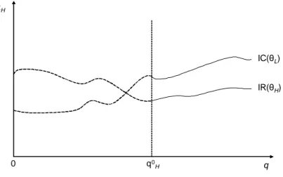
tH q q0 H IC( L) IR( H) 0
Figure 2. Case 1— the binding constraint when qH = qH0 is IR( H).
other type; otherwise separation would not occur. Constraint (iii), the IR( H) constraint,
imposes that the payo¤ of the agent who knows that the state is H cannot be lower than
his reservation value. For each quantity level qH, constraints IC( L) and IR( H) impose an
upper bound on the value of the up-front transfer tH:
Deriving the solution to Problem 2 o¤ers important insights regarding the crucial e¤ects leading to the existence of ine¢ cient equilibria, and we shall do so here.
In any solution to Problem 2, at least one of the constraints IC( L) or IR( H) is binding.14
Suppose that this were not the case; then it would be possible to increase tH by an arbitrarily
small amount > 0 and still have all the constraints in the problem satis…ed (including IC( H)) while increasing the objective function, which would be a contradiction.
Let us now be more speci…c about which of the constraints IC( L) or IR( H) is binding.
There are two possible cases, which I consider separately.
Case 1: The binding constraint when qH = qH0 is IR( H). This case is depicted in Figure 2.
When IR( H) is the binding constraint at qH = qH0, …rst-best investment and full surplus
extraction in both states L and H is incentive compatible. Therefore, the solution to
Problem 2 involves qH = qH0 and tH such that IR( H) binds. This implies that the payo¤ of
the principal of type H associated with the best separating allocation is the …rst-best total
surplus in state H, S(a0H; H), and bcH = (btH; qH0 ) where btH = UA(0; qH0; a (qH0; 1) j H). In
this case, there is no con‡ict between surplus extraction and e¢ ciency: the best separating allocation is characterized by full surplus extraction and full e¢ ciency in terms of the agent’s investment decision.
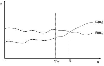
Case 2: The binding constraint when qH = qH0 is IC( L). This case is depicted in Figure 3.
To study the solution to Problem 2 in this case, I …rst analyze which constraint is binding for qH 2 [q0H; 1].
14Usually in this type of problem constraint IC(
H) is not binding. Therefore, it is omitted during the
determination of the solution to the problem and checked to be satis…ed ex-post. I do this in Appendix A (see Lemma 7).
tH q q0 H IC( L) IR( H) 0 q
Figure 3. Case 2— the binding constraint when qH = q0H is IC( L).
Lemma 4. Constraints IC( L) and IR( H) intersect only once in the interval [q0H; 1]. Denote
the intersection quantity by q. Then, IC( L) is the binding constraint for qH 2 [qH0; q] and
IR( H) is the binding constraint for qH 2 [q; 1].
Proof. See Appendix B.
Obtaining the solution to Problem 2 involves determining how the expected payo¤ of the principal of type H (the objective function) evolves with qH along the relevant binding
constraint.
For qH > q, the binding constraint is IR( H), so there is full surplus extraction and the
payo¤ of the principal is given by S(a (qH; 1); H). Observe that the expected total surplus
S(a (qH; 1); H) reaches its maximum value at qH = q0H, since a (qH0; 1) = a0H, which is the
…rst-best investment in state H. Therefore, from concavity of S(a; H) in investment a and
the fact that the agent’s investment decision a (qH; 1) is increasing in qH, it follows that
S(a (qH; 1); H) decreases in qH for qH q (recall that q qH0). Thus, the payo¤ of the
principal type H decreases with qH in the interval [q; 1] and therefore a solution to Problem
2 must satisfy qH q.
For qH 2 [qH0; q], the binding constraint is IC( L). To study how the expected payo¤ of
the principal of type H evolves with qH along the constraint IC( L), let m(qH) denote the
function obtained by substituting tH in the expected payo¤ of the principal of type H by
its value when constraint IC( L) is binding, i.e.,
m(qH) = UP(0; qH; a (qH; 1) j H) UP(0; qH; a (qH; 1) j L) + S(a0L; L).
Di¤erentiating it with respect to qH, we obtain
@m(qH) @qH = @ @qH [UP(0; qH; a (qH; 1) j H) UP(0; qH; a (qH; 1) j L)] + @ @a[UP(0; qH; a (qH; 1) j H) UP(0; qH; a (qH; 1) j L)] @a (qH; 1) @qH .
Changing qH has a direct e¤ect, which is given by the …rst term, and an indirect e¤ect
through investment that corresponds to the second term. The …rst term, which is equal to 1
2[E[vP j H] E[vP j L]] 0 in the case of private information about vP, and to
1
2[E[VE j L] E[VE j H]] 0
in the case of private information about VE, represents the direct surplus extraction e¤ ect :
by increasing qH, the principal of type H can also increase the up-front transfer tH in a
way that IC( L) continues to be satis…ed and her total payo¤ increases. This e¤ect stems
from the fact that when holding the agent’s investment …xed, the principal’s expected payo¤ exhibits the single crossing property with respect to transfer and quantity, i.e., the marginal rate of substitution between transfer and quantity is bigger for the principal of type H than
it is for the principal of type L. The second term, which represents the indirect investment
e¤ ect, is equal to
v0A(a (qH; 1))[Ps(a (qH; 1); H) Ps(a (qH; 1); L)]
@a (qH; 1)
@qH
and is also positive since @a (qH; 1)=@qH 0 (see Lemma 1) and Ps(a; H) Ps(a; L) for
all a 2 A. Intuitively, the investment e¤ect is positive because the payo¤ of the principal of type H is more sensitive to relationship-speci…c investment than the payo¤ of the principal
of type L. Therefore, it is the principal of type H who gains more by increasing quantity
and inducing the agent to invest more.
Since the direct surplus extraction e¤ect and the indirect investment e¤ect are both posi-tive, the expected payo¤ of the principal of type H increases with contracted quantity when
moving along the IC( L) constraint. This result, together with the fact that that payo¤
decreases with contracted quantity when moving along IR( H) when qH > q, implies that
the solution to Problem 2 is given by qH = q.15 Hence, in this case, the contract of the
principal of type H associated with the best separating allocation is bcH = (btH; q), where
btH is such that IR( H) binds. The payo¤ of the principal associated with this contract is
S(a (q; 1); H) < S(a0H; H).
In contrast to Case 1, in this case the outcome associated with the best separating allocation is ine¢ cient in terms of investment: in order to signal information to extract surplus, the principal sets an excessively high quantity (q > qH0), leading the agent to overinvest in the relationship. This completes the derivation of the best separating allocation. I now proceed to the characterization of equilibrium outcomes.
As argued above, following the proposal of a best separating allocation m = fbcb L;bcHg by
the principal, there is a continuation equilibrium in which the agent accepts the principal’s proposal and then the principal chooses contract bcL if she is of type L and contract bcH
15Since the expected payo¤ of the principal of type
H increases with quantity when moving along the
if she is of type H. Hence, the remaining question is whether both types of principal
proposingm = fbcb L;bcHg followed by this separating continuation equilibrium constitutes an
equilibrium of the overall game, i.e., whether there exist beliefs and continuation equilibria o¤-the-equilibrium path such that no type of principal gains by deviating and proposing a menu m0 6= bm. The next proposition clari…es this question. In what follows, let M denote the set of …nite menus of contracts and bUP( L) and bUP( H) denote the principal’s payo¤s—
derived above— associated with the best separating allocation.
Proposition 2. If both types of principal propose a menu m 2 M, followed by a continuation equilibrium (after menu proposal) in which the principal’s payo¤ s eUP( L) and eUP( H) are
such that eUP( j) UbP( j) for all j 2 fL; Hg, then there are o¤-the-equilibrium path beliefs
such that this proposal and continuation equilibrium constitutes an equilibrium outcome of the overall game.
Proof. See Appendix B.
Proposition 2 provides su¢ cient conditions for an equilibrium. Speci…cally, it ensures that both types of principal proposing a menu of contracts m, followed by a continuation equilibrium (after the menu proposal) in which the principal’s payo¤s Pareto dominate the payo¤s associated with the best separating allocation constitutes an equilibrium.
An implication of Proposition 2 is that both types of principal proposing the best separating allocation, followed by the respective separating continuation equilibrium, always constitutes an equilibrium of the game. In particular, Proposition 2 establishes that ine¢ cient equilibria exist. Among these are those in which the principal of type H distorts the contracted
quantity (relative to qH0, which is the quantity that induces the agent to invest e¢ ciently in state H) in order to extract more surplus from the agent.
This result is important not only because of the speci…c e¢ ciency implications that it has, but also because it emphasizes that surplus extraction and e¢ ciency of investment can in fact con‡ict with one another when parties contract under asymmetric information. I next allow exclusivity to be contractible and investigate its role in mitigating this con‡ict. 4.3. Quantity and Exclusivity Contracts. Suppose now that both quantity and exclu-sivity are contractible, i.e., Q = E = [0; 1]. In this case, a contract is triple c = (t; q; e). Because of the irrelevance result of Proposition 1, contractibility of exclusivity does a¤ect the set of equilibrium outcomes when the principal’s private information is about vP. Thus,
in this section only the case where the principal’s private information is about the external value VE is considered.
To characterize the equilibrium allocations and payo¤s, I start by presenting in Lemma 5 lower bounds for the principal’s equilibrium payo¤s. Then, in Proposition 3, I present the equilibrium payo¤s themselves and characterize equilibrium investments.
Lemma 5. Suppose that quantity and exclusivity are contractible (Q = E = [0; 1]). Then, in any equilibrium, the payo¤ of the principal of type j is at least the …rst-best expected total
surplus S(a0j; j), for all j 2 fL; Hg.
Proof. See Appendix B.
Contractibility of exclusivity plays no role in ensuring to the principal of type Lthe
…rst-best total surplus S(a0L; L). Under Condition 1, the principal of type L always achieves
this payo¤ even if exclusivity is not contractible. In contrast, in the case of the principal of type H, it is the fact that exclusivity is contractible that allows the principal to construct a
contract that guarantees her the …rst-best total surplus S(a0H; H). Note that, we have just
seen in the previous section that when exclusivity is not contractible, there exist equilibria in which the payo¤ of the principal of type H is S(a (q; 1); H) < S(a0H; H).
To illustrate the role of exclusivity when the principal is of type H, consider the expected
payo¤ of the agent given contract (t = 0; q; e), state and investment a. In the case of private information about the external value VE, this payo¤ can be written as
UA(0; q; e; a j ) =
1
2E[maxfV (a); VEg j ] 1
2[q(vP vA) + (1 q)(1 e)E[VE j ] (a): When the contract prescribes full exclusivity, i.e., e = 1, the agent’s expected payo¤ is a¤ected by only through the term 12E[maxfV (a); VEg j ]. Therefore, from the fact that
the distribution of the external value VE in state L…rst-order stochastically dominates that
in state H, it follows that
(13) UA(0; q; e = 1; a j L) UA(0; q; e = 1; a j H) for all a 2 A:
Intuitively, when the principal promises full exclusivity, the agent is better o¤ when the principal has a high outside option (state L), since he can appropriate part of it at the
renegotiation stage by threatening to enforce the contract and prevent the principal from trading with third parties:
From (13), it follows that the agent’s expected payo¤ UA(0; q; e = 1; a (q; bH) j bH) is
decreasing in his belief bH, for any given quantity q. In particular, this holds for q = q0H.
This implies that regardless of the agent’s beliefs, he always accepts contract (t; q0
H; e = 1)
in which t = UA(0; q0H; 1; a (q0H; 1) j H), i.e., his expected payo¤ when his beliefs are bH = 1
(his worst possible payo¤ across beliefs). Hence, exclusivity allows the principal to construct a contract in which the agent is better o¤ in state L than in state H: This is also possible
when exclusivity is not contractible if the principal sets a su¢ ciently high quantity in the contract. The problem in doing so, however, is that she distorts the agent’s investment decision.
Now I turn to the question of equilibrium payo¤s and investments.
Proposition 3. Suppose that quantity and exclusivity are contractible (Q = E = [0; 1]). Then, in any equilibrium, investment levels are e¢ cient (…rst-best in both states) and the
principal always appropriates the …rst-best total surplus, i.e., the equilibrium payo¤ of the principal in state j is S(a0j; j) for all j 2 fL; Hg.
Proof. Consider an equilibrium and let eUP( j) denote the principal’s payo¤ in state j in
that equilibrium. Lemma 5 implies that eUP( j) S(a0j; j) for all j 2 fL; Hg. Individual
rationality of the agent implies that it is not possible that eUP( j) S(a0j; j) for all j 2 fL; Hg
and, simultaneously, eUP( j) > S(a0j; j) for some j 2 fL; Hg. The two preceding results imply
that eUP( j) = S(a0j; j) for all j 2 fL; Hg. From individual rationality of the agent and the
fact that eUP( j) = S(a0j; j) for all j 2 fL; Hg, it follows that investment must be e¢ cient
(…rst-best) in both states Land H.
Proposition 3 establishes that in any equilibrium of the game when the principal can con-tractually use both quantity and exclusivity, the investment levels are e¢ cient in both states
L and H. To illustrate why e¢ ciency is always obtained when both quantity and
exclu-sivity are contractible (as opposed to the case when only quantity is contractible), consider the derivation of the best separating allocation in Case 2 presented in the previous section (see Figure 3). Recall that, in that case, investment is ine¢ cient due to the fact that the principal sets an excessively high quantity (q > qH0) in order to extract more surplus from the agent. When exclusivity is contractible, instead of increasing quantity above q0
H, which
induces the agent to overinvest in the relationship, the principal can set quantity qH0 and use (increase) exclusivity to move along the IC( L) constraint, signal her type and extract
surplus from the agent. Surplus extraction can be achieved in this way because the direct surplus extraction e¤ect associated with exclusivity is positive when the source of private information is the external. Moreover, exclusivity does not directly a¤ect the agent’s invest-ment decision, implying that surplus extraction through exclusivity does not interfere with provision of investment incentives.
The preceding analysis shows that, in contrast with the case of private information about internal values (Section 3), contractibility of exclusivity has important implications when private information is about external values. In particular, it shows that the ability to contractually use exclusive provisions eliminates ine¢ cient equilibria that may otherwise exist. I have therefore identi…ed a situation in which contractibility of exclusivity enhances e¢ ciency.
5. Conclusion
The literature on contractual solutions to the hold-up problem has focused on situations where the parties to the contract have symmetric information when contracting about future transactions. In this paper, I depart from this literature by examining a situation in which the party that designs the contract at the contracting phase has relevant private information. I show that because of information concerns, the contract designer may distort the contract’s terms relative to those that induce e¢ cient investment so as to signal information and appro-priate more of the surplus generated. I also show that when private information concerns the
value of trade with external parties, the ability to include exclusive clauses in the contract plays an important role in eliminating these distortions and, consequently, the ine¢ ciency of investment.
Regarding the literature on the e¤ect of exclusive contracts on relationship-speci…c in-vestment, the analysis in this paper complements that in Segal and Whinston (2000) and De Meza and Selvaggi (2007). Following a cooperative approach to model renegotiation, Segal and Whinston (2000) show that renegotiable exclusivity contracts have no e¤ect on relationship-speci…c investment. De Meza and Selvaggi (2007) point out that if the bargain-ing solution to renegotiation is non-cooperative, exclusivity may a¤ect relationship-speci…c investments. The present paper contributes to this literature by providing a novel chan-nel through which exclusive agreements a¤ect relationship-speci…c investments. Concretely, because exclusivity signals information, it helps to mitigate the con‡ict between signalling information and providing incentives to invest that is present when parties contract under asymmetric information.
On a more practical level, this paper o¤ers an explanation as to why contracts often specify simultaneously both a quantity to be traded in the future and an exclusivity clause. It also o¤ers an explanation as to why …rms voluntarily bind themselves by committing to trade exclusively with another …rm. Furthermore, the e¤ect of exclusivity that I highlight here may be important for policy design. The major (and unsettled) debate on that front is on whether exclusive agreements serve anticompetitive purposes and, as a consequence, on whether they should be contractually allowed. By showing that contractibility of exclusivity may enhance e¢ ciency of investment, this paper suggests that a policy that systematically prohibits exclusive contacts may be misguided.
Appendix
A. Auxiliary Results
Proposition 4. A best separating allocation m = fbcb L;bcHg is incentive compatible given the
separating beliefs.
Proof. I only show here that given separating beliefs the principal of type H prefers to
choosebcH instead of bcL. The proof that the principal of type L prefers to choosebcLinstead
of bcH is perfectly analogous. Let fbcL; cHg be a solution to the problem presented in (12)
for the principal of type L. First, because fbcL; cHg must satisfy the IC( H) constraint
in the problem, we obtain that UP(cH; a (cH; 1) j H) UP(bcL; a (bcL; 0) j H). Second,
because the constraints of the problem presented in (12) are exactly the same whether we are solving it for the principal of type L or for the principal of type H, fbcL; cHg is also a
feasible menu in the problem for the principal of type H. This immediately implies that
UP(bcH; a (bcH; 1) j H) UP(cH; a (cH; 1) j H). From this inequality and the fact shown
above that UP(cH; a (cH; 1) j H) UP(bcL; a (bcL; 0) j H), it follows that UP(bcH; a (bcH; 1) j H) UP(bcL; a (bcL; 0) j H).
Lemma 6. Both when private information is about vP and when private information is about
VE, UA(t; q = 1; e = 0; a j L) UA(t; q = 1; e = 0; a j H) for all t 2 R and all a 2 A:
Proof. By taking expectations of (1), we obtain that UA(t; 1; 0; a j ) =
1
2E[maxfV (a); VEg j ] 1
2E[vP vA(a) j ] (a) t:
Because does not a¤ect vA(a), we obtain that UA(t; q = 1; e = 0; a j L) UA(t; q = 1; e =
0; a j H) if and only if
(14) E[maxfV (a); VEg vP j L] E[maxfV (a); VEg vP j H].
When private information is about vP, (14) follows directly from the fact that maxfV (a); VEg
vP is a decreasing function of vP and FvP[: j H] …rst-order stochastically dominates FvP[: j
L]. When private information is about VE, (14) follows directly from the fact that maxfV (a); VEg
vP is an increasing function of VE and FVE[: j L] …rst-order stochastically dominates FVE[: j
H].
Lemma 7. The proposed solution to Problem 2 (ignoring constraint IC( H)), i.e.,
con-tract bcH = (btH = UA(0; q0H; a (qH0; 1) j H); q0H) if Case 1 holds and contract bcH = (btH =
Proof. I …rst prove the result for Case 1, i.e., that UP(bcL; a (bcL; 0) j H) UP(bcH; a (bcH; 1) j H) when bcH = (btH; qH0) with btH = UA(0; qH0; a (qH0; 1) j H). Recall that contract bcL =
(btL; q0L) with btL= UA(0; qL0; a (qL0; 0) j L). The result is established by noting that
UP(bcL; a (bcL; 0) j H) = UP( 0; q0L; a (q0L; 0) H) + UA( 0; qL0; a (qL0; 0) L)
UP( 0; q0L; a (q0L; 0) H) + UA( 0; qL0; a (qL0; 0) H)
= S(a (q0L; 0); H)
S(a0H; H) = UP(bcH; a (bcH; 1) j H);
where: (i) the …rst equality follows from the fact that UP(t; q; a j ) = UP(0; q; a j ) + t for
all q 2 [0; 1], a 2 A and t 2 R; (ii) the …rst inequality follows from Condition 1; (iii) the second equality from (3); (iv) the second inequality from the fact that a0H is the investment level that maximizes S(a; H); and (v) the last equality from (3) again.
I now prove the result for Case 2, i.e., that UP(bcL; a (bcL; 0) j H) UP(bcH; a (bcH; 1) j H) when bcH = (q; btH) with btH = UA(0; q; a (q; 1) j H). I do this by comparing both
UP(bcH; a (bcH; 1) j H) and UP(bcL; a (bcL; 0) j H) with UP(ecH; a (ecH; 1) j H), where ecH =
(etH; q0L) with etH such that ecH satis…es constraint IC( L) of Problem 2 with equality.
(1) Comparing UP(bcH; a (bcH; 1) j H) with UP(ecH; a (ecH; 1) j H). Because the expected
payo¤ of the principal of type H increases when moving along the IC( L) constraint by
increasing quantity q (see the derivation of the solution to Problem 2 in Section 4.3) and contractbcH = (q; btH) (where q > qL0 ) also satis…es constraint IC( L) with equality, we obtain
that
(15) UP(bcH; a (bcH; 1) j H) UP(ecH; a (ecH; 1) j H).
(2) Comparing UP(bcL; a (bcL; 0) j H) with UP(ecH; a (ecH; 1) j H). By construction, ecH
satis…es constraint IC( L) with equality. Thus UP(ecH; a (ecH; 1) j L) = UP(bcL; a (bcL; 0) j L),
which is equivalent to
btL etH = UP( 0; qL0; a (qL0; 1) L) UP( 0; qL0; a (qL0; 0) L).
This means that btL etH is identical to the incremental payo¤ to the principal of type L
associated with an increase in investment from a (q0L; 0) to a (q0L; 1). From Lemma 2, it follows that
btL etH UP(0; q0L; a (q0L; 1) j H) UP(0; qL0; a (qL0; 0) j H),
which is equivalent to
(16) UP(ecH; a (ecH; 1) j H) UP(bcL; a (bcL; 0) j H).
From (16) and (15) it follows that UP(bcL; a (bcL; 0) j H) UP(bcH; a (bcH; 1) j H).
Lemma 8. Suppose that IC( L) is the binding constraint in Problem 2 when q = qH0 (Case
2). If a contract c = (t; q) satis…es simultaneously UP(c; a (c; 0) j L) S(a0L; L) and
Proof. Given a contract c = (t; q), conditions UP(c; a (c; 0) j L) S(a0L; L) and UP(c; a (c; 0) j H) > S(a (q; 1); H) are equivalent to
(17) S(a (q; 1); H) UP(0; q; a (q; 0) j H) < t S(a0L; L) UP(0; q; a (q; 0) j L).
Therefore, they hold simultaneously only if in (17) the term on the right side of t is greater than that on the left side. That is, only if
(18) S(a (q; 1); H) S(a0L; L) < UP(0; q; a (q; 0) j H) UP(0; q; a (q; 0) j L).
Since by Lemma 2 the right-hand side of (18) is an increasing function of q, it su¢ ces to show that condition (18) is not satis…ed when q = q. To obtain this, note that
S(a (q; 1); H) S(a0L; L) = UP(0; q; a (q; 1) j H) UP(0; q; a (q; 1) j L)
UP(0; q; a (q; 0) j H) UP(0; q; a (q; 0) j L),
where: (i) the …rst equality is obtained by using the fact that S(a (q; 1); H) = UP(0; q; a (q; 1) j H)+UA(0; q; a (q; 1) j H) and the fact the incentive compatibility of type Lis binding in the
best separating allocation, i.e., S(a0L; L) = UP(0; q; a (q; 1) j L)+UA(0; q; a (q; 1) j H); and
(ii) the inequality follows from the fact that UP(0; q; a (q; bH) j H) UP(0; q; a (q; bH) j L)
is an increasing function of bH, which is an implication of Lemma 2: This completes the proof
of the Lemma.
B. Proofs of Propositions and Lemmas in the Main Text
Proof. (of Proposition 1) Using the fact that investment and information a¤ect only internal values, the expected payo¤s of the principal and the agent, given contract c = (t; q; e) and agent’s beliefs bH, can be written as:
(19) UP( c; a (c; bH) j ) = 1 2E[maxfV; VEg + q(vP vA) j ; a (c; bH)]+ +12(1 q)(1 e)E[VE] + t; 2 and UA( c; a (c; bH) j bH) = (1 bH) 1 2E[maxfV; VEg q(vP vA) j L; a (c; bH)] (20) +bH 1 2E[maxfV; VEg q(vP vA) j H; a (c; bH) ] 1 2(1 q)(1 e)E[VE] (a (c; bH)) t,
where a (c; bH) is as de…ned in (4). Notice that the agent’s payo¤ from investment is
ad-ditively separable from both the exclusivity term e and the transfer t. Thus, the agent’s investment decision does not depend on e and t, so instead of a (c; bH) we can simply write
a (q; bH). From this observation and direct inspection of (19) and (20), we obtain that for the
same beliefs bH, contracts c = (t; q; e) and c0(c) = (t0; q0; 0) 2 C0 with t0 = t 12(1 q)eE[VE]
and q0 = q, generate the same expected payo¤s to the principal (in both states L and H)