Cointegration analysis : gilt-equity yield ratio in pigs and Germany (econometric study using VAR/VECM methodologies)

(1)

COINTEGRATION ANALYSIS – GILT-EQUITY YIELD RATIO IN

PIGS AND GERMANY

(econometric study using VAR/VECM methodologies)

Mónica Filipa Moreira da Silva

Project submitted as partial requirement for the conferral of Master in Finance

Supervisor:

Prof. José Dias Curto, ISCTE Business School, Departamento de Métodos Quantitativos

(2)

I

Resumo

The Gilt-Equity Yield Ratio (GEYR) tem-se mostrado uma ferramenta importante para os analistas de mercados na tomada de decisão, quanto à compra e venda de ações vs obrigações, mostrando-se um rácio sensível a situações de misprincing. Deste modo, o objectivo do estudo, passa pela análise da existência de cointegração do GEYR entre os PIGS e a Alemanha, averiguando se resultados estão condicionados pela situação económica de cada país.

O estudo apresenta duas metodologias para o cálculo do rácio: a primeira utiliza como denominador do rácio o dividend yield índex e a segunda utiliza os earnings yield índex. Utilizando como numerador comum bond yield. Para o período em análise, constatou-se que a estratégia predominante nas duas metodologias é “comprar ações”.

Considerando a primeira metodologia de cálculo do rácio, foi verificada a existência de cointegração do GEYR entre os países Portugal, Irlanda, Grécia, e Espanha. De acordo com a segunda metodologia a hipótese de cointegração do GEYR não é constatada para nenhum dos países. Concluindo-se que para esta metodologia de cálculo, a análise da relação do GEYR entre os países não é útil para uma tomada de decisão. Por sua vez, a Alemanha não está cointegrada (em ambas as metodologias) com nenhum dos PIGS, indicando-nos que o rácio não se mostrou uma boa ferramenta para analisar países com situações económicas diferentes.

A causalidade de Granger é também testada para as séries estacionárias em nível, (as quais se verificam apenas na segunda metodologia) concluindo-se, deste modo, não existir relação de causalidade entre as séries.

Palavras-chave: Rácio “Gilt-Equity Yield”, regras de decisão, não estacionariedade,

cointegração, Modelo Vetorial de Correção de Erros.

JEL Sistema de Classificação:

C32 - Time-Series Models; Dynamic Quantile Regressions; Dynamic Treatment Effect Models; G01 - Financial Crises;

(3)

II

Abstract

The Gilt-Equity Yield Ratio (GEYR) has been displayed as an important tool for market analysts on decision making as to the buy and sell of equities vs. bonds, being a sensitive ratio to “mispricing” situations. Therefore, the goal of this study is to check the existence of cointegration of the GEYR between PIGS and Germany, by examining whether the results are conditioned by the economic situation of each country.

This study shows two methodologies for the computation of the ratio: the first uses as ratio denominator the dividend yield index and the second uses the earnings yield index. We use as the common numerator the bond yield. It is eminent that the predominant strategy in both methodologies is to “buy equities”.

Considering the first methodology of the ratio computation, the existence of cointegration of the GEYR between Portugal, Ireland, Greece and Spain was verified. In conclusion, according to the second methodology, the cointegration hypothesis of the GEYR is not found in any of the countries, inferring that the GEYR comparison between countries is not useful for decision making. On the other hand, Germany is not cointegrated (in both methodologies) with any country of PIGS and that indicates that the ratio did not present to be a good indicator to analyze countries with different economic situations.

The Granger causality is also tested to the stationary series in level (which are only verified in the second methodology), concluding that there is no causality relationship between them.

Keywords: Gilt-Equity Yield Ratio, trading rule, nonstationarity, cointegration, VECM.

JEL Classification System:

C32 - Time-Series Models; Dynamic Quantile Regressions; Dynamic Treatment Effect Models; G01 - Financial Crises;

(4)

III

Acknowledgments

First of all, I am most grateful to my supervisor, Prof. José Dias Curto, for his guidance that helped me out immensely during this thesis work and for helping me choosing a theme that became very interesting to me. Also, he was an active guide who has shown attentiveness for the development of the thesis, aiding me in the resolution of emerging problems. Secondly, I also wanted to express my gratitude to Prof. Pedro Leite Inácio who assisted me in the analysis of some financial concepts, mainly in the understanding of the ratio under study.

Another special thank I would like to give is to my colleagues because they provided me assistance with some helpful comments on technical issues, especially to Vitor Brito for his availability to review the text.

I would like to thank Jacqui Neale who welcomed me in her house, providing me familiar sheltering and for her friendship, during my stay in the United Kingdom when I was in the research phase for my thesis.

And last, but certainly not the least, I would also like to thank to my family, for their patience, comprehension and for their support in everything I do, particularly during my graduation degree in Finance.

(5)

IV

List of Tables

Table 1: Strategy Decision with the GEYR results (using dividends yield index) ... 18

Table 2: Strategy Decision with the GEYR1 results (using earnings yield) ... 18

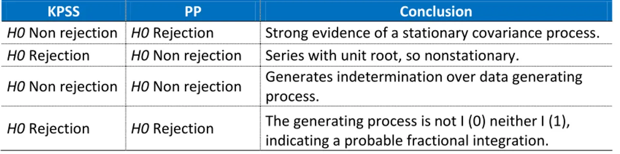
Table 3: Results combination of the KPSS and PP tests ... 28

Table 4: Data set to calculate GEYR ... 42

Table 5 – Description of variables ... 43

Table 6 – Trading decisions for different timeslots: 1st methodology (GEYR) ... 45

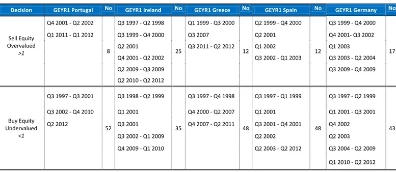
Table 7 – Trading decisions for different timeslots: 2nd methodology (GEYR1) ... 48

Table 8- Descriptive Statistics of GEYR (using dividend yield) ... 51

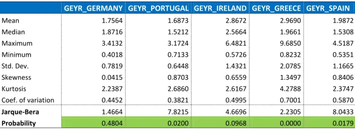
Table 9 - Descriptive Statistics of GEYR1 (using earnings yield) ... 52

Table 10 - Unit root tests (1st methodology) - GEYR ... 56

Table 11 - Unit root tests (2nd methodology) – GEYR1 ... 59

Table 12- Summary of the series behavior ... 61

Table 13 – Choosing of the Optimal Lag ... 62

Table 14- Bivariate cointegration for 1st methodology GEYR ... 63

Table 15- Number of cointegration vectors of Johansen tests ... 64

Table 16- Bivariate cointegration for 2nd methodology GEYR1 ... 65

Table 17- Bivariate VEC Model ... 67

Table 18 – Summary of cointegrated variable combinations ... 69

Table 19 – Series combinations that will be tested through Pairwise Granger causality tests. ... 70

(8)

VII

List of Figures

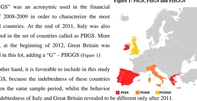
Figure 1- PIGS, PIIGS and PIIGGS ... 39

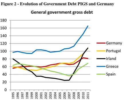
Figure 2 - Evolution of Government Debt PIGS and Germany ... 40

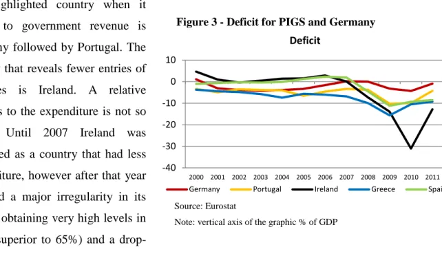
Figure 3 - Deficit for PIGS and Germany ... 41

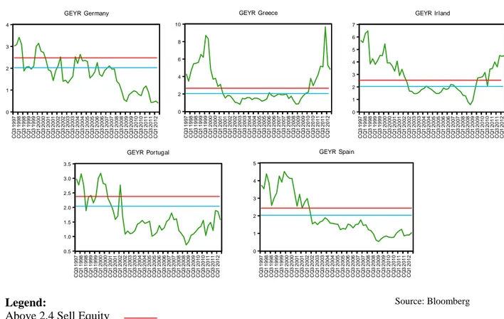
Figure 4 - Evolution of GEYR for the five countries being studied ... 44

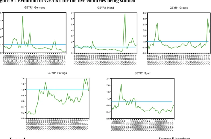
Figure 5 - Evolution of GEYR1 for the five countries being studied ... 46

Figure 6 – Original series of GEYR of Germany, without extreme point. ... 47

Figure 7 – Graphics of the studied series’ logarithms - 1st methodology ... 53

Figure 8 – Graphics of the studied series’ logarithms - 2nd methodology ... 53

Figure 9 - Evolution of the series’ logarithms of the GEYR for all countries – 1st methodology . 54 Figure 10 – Evolution of the series’ logarithms of the GEYR for all countries – 2nd methodology ... 54

Figure 11 – Graphics of the first differences of logarithms of the series ... 58

Figure 12 - Graphs of the first differences of logarithms of the series ... 60

List of Annex

Annex 1 - Economic Indicators - Government Revenues and Expenditures ... 79

Annex 2 - GEYR computation for five countries using two methodologies ... 80

Annex 3 - Optimal Lag: Outputs Eviews ... 82

Annex 4 - Cointegrations tests: Output Eviews ... 88

Annex 5 - VECM Outputs Eviews ... 92

(9)

VIII

Basic Notation

ADF Augmented Dickey-Fuller (unit root test)

AEG Aumented Engle-Granger

AIC Akaike's information criterion

AR Autoregressive

BEYR Bond-Equity Yield Ratio

Cov Covariance

DF Dickey-Fuller

DPS Dividends per stock

DSP Difference Stationary Process

DW Durbin Watson

ECM Error Correction Model

EG Engle-Granger

EPS earnings per stock GEYR Gilt-Equity Yield Ratio

KPSS Kwiatkowski, Phillips, Schmidt and Shin (test)

L Lag operator

N(μ, σ2) Univariate normal distribution with expected value μ and variance σ2 OLS Ordinary Least Square

PP Phillips-Perron (unit root test) PIGS Portugal, Ireland, Greece and Spain R2 Coeficiente de determinação

SIC Schwartz information criterion TSP Trend Stationary Process VAR Vector Autoregressive

Var Variance

VECM Vector Error Correction Model

(10)

1

1. Sumário Executivo

É evidente o crescente desenvolvimento de análises relacionadas com mercados financeiros, principalmente na vertente do mercado bolsista. A procura por indicadores sinalizadores de estratégias eficientes do mercado é cada vez mais notória, levando a uma necessidade sistemática de desenvolvimento de investigação nesta área. Os mercados bolsistas são de extrema importância para as economias, uma vez que são uma das principais formas de financiamento das empresas, permitindo assim a expansão dos seus negócios. Esta vantagem aparece associada à liquidez das ações, passíveis de aquisição e de venda frequente, oferecendo uma liquidez superior a outros investimentos como o imobiliário ou arte. A evolução do mercado de ações é representativa da dinâmica de uma economia, e normalmente, o crescimento dos mercados acionistas, está associado ao aumento do investimento empresarial e da confiança dos consumidores.

Tendo em conta a importância deste tipo de mercados, sentiu-se a necessidade de estudar um rácio que permitisse relacionar os rendimentos do investimento em obrigações e ações - o chamado Gilt–Equity Yield Ratio (GEYR), visando perceber os movimentos dos mercados e quais as suas tendências de investimento, se preferencialmente ações ou pelo contrário, obrigações. A componente diferenciadora desta dissertação, evidencia-se perante a carência de estudos, que simultaneamente analisem o rácio e investiguem a existência de cointegração do GEYR entre países.

Deste modo, testa-se a existência de uma relação de equilíbrio de longo prazo do GEYR para os países Portugal, Irlanda, Grécia, Espanha (PIGS) e Alemanha, considerando-se duas metodologias de cálculo. A primeira consiste no rácio entre bond yield e dividend yield índex e a segunda considera o rácio entre bond yield e earnings yield index. Toda a informação necessária para o seu cálculo foi retirada dos índices bolsistas de cada um dos países em estudo. Os resultados obtidos para o cálculo do rácio indicam, que para o período em análise (períodos trimestrais de 1997 a 2012) a estratégia predominante em ambas as metodologias para a generalidade dos países é “buy equities”. Visando mostrar que as ações dos índices representativos de cada país estão subavaliadas.

(11)

2 Para a primeira metodologia, os testes de análise de raízes unitárias/estacionariedade ADF, KPSS e PP, evidenciam a não estacionariedade do GEYR para todos os países, na segunda metodologia verifica-se a estacionariedade do GEYR para Portugal, Irlanda e Grécia.

A aplicação do teste de cointegração de Johansen e, posteriormente a aplicação do modelo vetor de correção de erro (VECM), aplicado às séries que se evidenciaram cointegradas, indica-nos que efetivamente existe cointegração entre as séries, apenas na a primeira metodologia de cálculo abordada. De acordo com uma análise bivariada verifica-se que o GEYR de Portugal (variável dependente) está cointegrado com o GEYR da Irlanda assim como com a Grécia e o GEYR da Grécia (variável dependente) está cointegrado com o GEYR de Portugal assim como com a Espanha. Outra análise interessante é que a cointegração também é verificada entre o GEYR de Espanha (variável dependente) e o GEYR de Portugal. Contudo, quando consideramos o GEYR de Portugal como a variável dependente, através da análise do teste VECM, verifica-se que a estimativa do coeficiente da equação de cointegração não é estatisticamente significativa.

Na segunda metodologia, as únicas séries que se revelam não estacionárias, em nível com a mesma ordem de integração, são o GEYR da Alemanha e Espanha. Estas séries evidenciaram-se não cointegradas, sendo que, todas as regressões que se possam efetuar entre elas incorrem em relações espúrias, isto é, relações sem sentido, não proporcionando ao investidor uma análise eficiente.

A aplicação dos testes de causalidade de Granger às séries estacionárias em nível, (na segunda metodologia) para Portugal, Grécia e Irlanda indicam que, efetivamente, não se verifica uma relação de causalidade. Assim sendo, não faz sentido procedermos à estimação dos coeficientes dessa regressão, através do modelo vetor autoregressivo (modelo VAR). Não existindo uma dependência de curto prazo entre as variáveis, o investidor também não deve considerar uma análise sincrónica deste rácio entre os países mencionados.

A contribuição deste estudo para a literatura econométrica e financeira, visa evidenciar que, utilizando a segunda metodologia de cálculo, o GEYR não se revela um bom indicador para uma comparação entre os países. Uma vez que não foram encontradas evidências de uma relação de dependência tanto de curto, como de longo prazo entre as séries. Por outro lado, a primeira metodologia abordada para o cálculo do rácio revela-se bastante interessante numa análise de

(12)

3 longo prazo, entre os países com situação económica idêntica, pois a evidência de cointegração é notória. Ainda assim, salienta-se o facto da cointegração do GEYR não ser verificada em todos os países dos “PIGS”. Outra conclusão evidente é que o GEYR da Alemanha nunca se mostra cointegrado com o GEYR dos denominados PIGS, devido à situação económica da Alemanha ser mais estável comparativamente à situação económica que os PIGS enfrentam.

Nesta dissertação, não foi possível o desenvolvimento do estudo das propriedades de relacionamento da cointegração, inerentes às variáveis contempladas na equação de cointegração. No entanto, num futuro estudo poderá ser bastante interessante a aplicação dos testes de exogeneidade, de assimetria e de proporcionalidade às diferentes variáveis em estudo.

(13)

4

2. Introduction

Since the 1990s there is a great skepticism by the academic about traditional ratios that evaluate stocks and bonds, like the traditional dividend yield ratio (D / P) or price-to-earning (P / E) ratios. Financial ratios present some limitations. In the case of the dividend yield ratio, its variation relies heavily on companies’ information disclosure, thereby presenting restrictions to those who have not access to this kind of information. On the other hand, the precaution to take with earnings ratio is essentially due to the stock price which is based on numerous factors besides net income, like an industry-wide drop in revenue prospects. There are also legal actions against the company, healthy-publicized warranty claims, the existence of valuable patents and so much more.

Loss of confidence in this type of ratios is easily noticeable majorly in periods of crisis since the financial stabilization policies impacts on financial markets volatility, thereby adding uncertainty to the investments. Throughout the years it has been shown that the analysis of these ratios could not be restricted to mere historic data, because they reflect structural breaks that occur on external factors, such as political, economic and/ or financial, differing in each country coming from periods with more instability and they should be analyzed in detail and individually.

With this all said, due to that loss of confidence in traditional ratios, it was considered the need of finding a ratio that gathered financial securities – stocks and bonds – and capable of sustaining more consistently trading decisions of the investors. In recent years, as a result the financial community redirected its attention to an 'enhanced' evaluation ratio, the Gilt-Equity Yield Ratio (GEYR). According to Clare, Thomas and Wickens (1994) it is a key indicator to know if the investment should be made on stocks or bonds. In Portugal, the GEYR is still a much underutilized ratio since the investors continue to base their decisions on traditional ratios. In countries like the UK and the USA it is becoming more and more used in order to ensure efficiency in investments made on the capital markets. It is also important to refer that the designation GEYR was developed by the British authors/researchers and it is often designated as BEYR (Bond-Equity Yield Ratio).

There are some studies that analyze this ratio and according to Mills (1991) the GEYR was an extremely valuable ratio for the market practitioners in the UK in order to estimate future

(14)

5 movement in prices. After three years Clare et al. (1994) used GEYR as a driver for investment decisions and evaluated three different trading rules between 1990 and 1993. The authors conclude that GEYR is a beneficial predictor of equity returns.

Levin and Right (1998) strained the work of Clare et al. (1994) and they found, through a wide sample of 14 years (1982-1996) that the GEYR by itself is not capable of providing a profitable asset allocation decision criterion. Lastly Harris and Sanchez-Valle (2000) and Brooks and Persand (2001) recommended that the Gilt-Equity Yield Ratio had considerable explanatory power for the UK equity returns.

Giot and Petitjean (2004) used the BEYR to investigate the long term relationship between stock index prices, dividends and bond yields. By using a wide sample of 7 countries (Germany, Belgium, France, Japan, The Netherlands, the UK and the US) between 1973 and 2004, the authors empirically investigated their molds by using first cointegration analysis and then they stretched Brooks and Persand’s regime exchanging approach by adding another trading rule. Giot and Petitjean made clear that a long-term cointegrating relationship subsists between stock index earnings, stock index prices and government bond yields.

It is notorious the lack of articles and studies about the GEYR that contemplate international relationships ascertaining the existence of long-term relationships between the countries (cointegration), so it becomes interesting to understand through joint analysis of securities (stocks and bonds) the behavior of one country facing another. This thesis is a pioneer, because it contemplates countries that were never considered so far (such as Portugal) and that are living a similar period of economic and financial recession (except for Germany) and also for the fact of the GEYR is being calculated through two methodologies (which will be described a posteriori). Due to the lack of empirical research, the thesis aims to present a synthesis of the econometric models that allows us to explain the relationship that could exist between GEYR in the set of countries named PIGS and Germany. Can we conclude that Germany GEYR is related with the same ratio of Portugal, Ireland, Greece and Spain? This is the main question that we want to answer.

Having said this, the goal of this thesis is in an initial phase to compute the GEYR and analyze its results to Portugal, Greece, Italy, Ireland and Germany and according to the historical data

(15)

6 comprehend the investment trend, whether if it is stocks or bonds in each country. After the ratio calculus it will be studied the behavior of the series individually to understand if they are stationary or not, applying the unit root test (ADF test) and other common tests to conclude about the stationarity of the series (KPSS and PP). For the series that initially present themselves stationary (series in levels) we use the Granger causality test to understand if the results of the GEYR in one country have any causality relationship with the GEYR results in another country. After the Granger causality analysis, it will be estimated the VAR model in order to obtain the short-term dependencies.

Finally, to the series that are nonstationary it is applied the cointegration tests in order to determine the existence of long-term relationships of the GEYR between countries and for that it is used the Jonhasen method along with the VECM, in order to estimate the coefficients of the cointegrating equations in the long and short terms. In order to achieve the outlined goals, to apply and estimate different econometric models methodologies, we use Eviews software.

The study is organized as it follows: in chapter two it is presented a brief literature review to describe modeling and cointegration techniques to better understand how the GEYR is modeled and estimated; in the third chapter we describe and explain how the GEYR can be computed. In this study, the ratio is computed with the first input earnings yield index and bond yield and subsequently with the dividend yield index and bond yield. Chapter four describes briefly the methodology under the GEYR analysis, especially econometric cointegration techniques. Data analysis and empirical results are presented and discussed in chapter five. In this chapter we analyzed the series behavior for each country and we test the stationarity of the series. Subsequently, the cointegration test is applied to nonstationary series. The critical analysis generated by each output and the presentation of cointegrating equations will be done in this chapter as well. Finally the conclusions and main contributions of this study are presented in Chapter 6.

(16)

7

3. Literature Review

In this chapter we present a brief literature review about the development of the Gilt-Equity Yield Ratio (GEYR) and we discuss also some of the econometric methodologies that will be applied to the ratio. In this analysis the main subjects are: The GEYR Development, Stationarity, Granger Causality and Cointegration.

Until the year 1994 there were some studies related with existing movements on the market that analyzed variables like stocks, bonds, and dividend yields, amongst others. Until this time the GEYR had not yet been developed. There are lots of papers and investigations about the variations that occurred on the capital markets and we just refer a few on this thesis in order to frame the GEYR in the financial literature. In this literature review it is important to mention studies that aid understanding not only the principal theme, but all its implications. Down below there is a brief description of the withdrawn analysis from the articles related with the stock, bonds and interest markets, amongst other financial securities along with an econometric approach.

Chen, Roll and Ross (1986) investigated the influence of inflation on interest rates (short and long-term), on production growth, on real consumption growth and consequently they verified the impact of those variations on the return of US stocks. The main conclusion is that a raise on internal production increases significantly the excess returns, whilst a raise on inflation reduces it. After this study, Giovannini and Jorion (1987) evidenced that the excess returns are negatively correlated with the nominal interest rate and stocks volatility presents a positive correlation with the nominal interest rate. In 1991 came Chen reaffirming the previous study, but he considered the correlation between more variables demonstrating the excess returns are negatively related to real economic growth and positively related to future economic growth.

Sentana and Wadhwani (1989) and Campbell and Hamao (1989) evidenced that equity returns in Japan can be predicted by using equity market dividend yield and an equivalent set of Japanese interest rates and yields spreads. Another study developed by Shah and Wadhwani (1990) mentions that through predictive power of the dividend yield and the term structure of interest rates for equity returns in 15 countries, the obtained results in the US should not be generalized to other countries, except for the UK, because markets work on distinct ways. Contrasting to Shah

(17)

8 and Wadhwani’s (1990) results, Clare and Thomas (1992) found that several yields spread together with other 'technical' variables and that increased the predictive power for German, Japanese, British and American equity and government bond markets during the 1980s.

The concept of correlation was widely investigated as we already verified in article from Giovannini and Jorion (1987) previously described. That investigation process led to the need of developing studies of cointegration in order to analyze determined characteristics of series that correlation do not allow us (e.g. long-term relationships between variables). Some studies will be highlighted throughout the next paragraphs related to the cointegration development. Cointegration analysis started being developed over 20 years ago by Granger (1981), Engle and Granger (1987) and Granger and Hallman (1991) contributions. They can reveal regular stochastic trends in financial time series data and that cointegration can be useful for long-term investment analysis. It has been proven by Granger and Hallman (1991) that investment decisions based only on short-term returns are inadequate, so it is important to consider the long-term relationships of asset prices. They also demonstrate that Hedge strategies established on correlation require constantly portfolio rebalancing, whilst strategies strictly based on cointegration do not need this rebalancing.

Bierens (1997), Park and Phillips (1988, 1989), Phillips and Hansen (1990), Saikkonen (1991), Sims et al. (1990) or Stock and Watson (1988) contributed to the development of approaches that can be considered an analysis of cointegration. Those approaches can be divided in parametric or non-parametric modeling. A non-parametric approach goes back to the theory developed by Engle and Granger (1987)1. The core of this approach is only on testing and estimating cointegration relationships, whilst all other characteristics of data generating process are processed as nuisance parameters. There are other authors for the parametric approach and the most popular is Johansen (1995). Other authors who deserve equal spotlight and also considered in this dissertation are Dickey and Fuller (1979) that concentrate their studies on the existing hypothesis of a unit root.

1

Clive W.J. Granger and Robert F. Engle shared a Nobel Prize in Economics in 2003. One of the contributions for which they have been awarded was cointegration. The second awarded contribution is the so-called ARCH models that allows to model time-varying conditional variances, a pertinent phenomenon in e.g. financial time series. Note as a historical remark that several other researchers were also 'close to discovering' cointegration around the same time, e.g. Box and Tiao (1977) and Kräamer(1981).

(18)

9 One of the studies that involved the concept of cointegration along with stocks and bonds was Wainscott’s (1990). He who used monthly returns of the US common stocks and long-government bonds examined the existing correlation between the two variables. The sample period lasted between January of 1925 and June of 1988. He calculated the correlation between bond yields and stocks using temporal horizons of 1, 2, 5 and 10 years. The main conclusion is that the correlation was unstable. Thus, if correlations are used for asset allocations, yield forecasts will be imprecise. In fact, correlation versus cointegration was also piece of work of several articles and according to Alexander and Dimitriu (2002), the use of cointegration for long-term inferences does not forbid the use of correlation as a short-term guide. For instance, short-term correlation can be utilized as a stock selection technique followed by a portfolio optimization based on cointegration.

According to Alexander (1999), the cointegration technique for time series modeling is common in financial markets applications. This author states that, a multivariate system will provide important information about the equilibrium price of financial assets and causality of returns within the system. Arbitrage between spot prices and future prices, modeling the structure of the yield curve, negotiations through a construction of “index tracking” and spreads, these are some of the applications of cointegration reviewed by the author in the article. It presents an international cointegrated portfolio model of stocks utilized for hedging within the European countries, Eastern Europe and Asia.

Opposing to the traditional strategies of “index tracking” and long-short equity based on correlation, Alexander and Dimitriu (2002) executed the optimization of a portfolio based on cointegration. They used it as a negotiation strategy based on index tracking that aims to replicate a reference source of market accurately in terms of returns and volatility. They also use cointegration to determine a neutral strategy of long-short equity market: aiming to minimize volatility and generate stable returns over all circumstances of the market. To validate its applicability, they took stocks of the Dow Jones Index Average (DJIA) and the presented results, strongly justifying, the use of cointegration to determining financial assets allocation.

More recently, Dunis and Ho (2005) equally used the cointegration concept to derivate a quantitative portfolio of European stocks in the context of two applications: the classical strategy of index tracking and the neutral strategy of long-short equity market. They use the data of the

(19)

10 Index Dow Jones EUROStoxx50 and its constituents stocks, within the period from 04-01-1999 to 30-06-2003. Still, the presented results improve the cointegration technique to the assets allocation, i.e. the results show that the designed portfolios are strongly cointegrated with the benchmark and indeed demonstrate good tracking performance.

Afterwards and using recent econometric methods in empirical research about relationships between stock prices, bond yields and dividend yields came the authors Mills (1991) and Clare, Thomas and Wickens (1994). The main goal of these authors was to verify empirically if there were a stable relationship between bond yields and dividend yields that could be used by the portfolio analysts to determine the attractiveness of equities comparing to the investment on bonds. Mills (1991) still developed another study that tested the existence of cointegration between equity prices, dividends and bonds and used the logarithms of the variables through observations at the end of each month since January of 1969 until May of 1989. These observations were removed from Financial Times Actuaries 500 equity index, the associated dividend index and the Par yield on twenty-year British Government stocks. The main conclusions to retain from this study is that Mills evidenced that each series was integrated of order 1 and posteriorly estimated the error correction model between stock prices, dividends and bond yields. After applying the necessary tests to this estimation, Mills found evidences about the existing long-term stable relation between bond yields and dividend yields.

However, in spite of this vast number of empirical studies related with financial markets, few analyzed the relationship between stocks and bonds simultaneously, verifying short and long-term relationships in each of these financial securities.

Due to this Clare, Thomas and Wickens (1994) estimated a ratio which contemplated gilt yields over dividend yields, calling it Gilt-Equity Yield Ratio (GEYR). In this study they realized that when the GEYR assumes big values, bonds should be purchased and consequently a low value of the GEYR means that bonds should be sold.

After this study others have been produced in financial markets literature. Next, we refer a few of them. Clare et al. (1994) used the GEYR to assure more efficient investment decisions evaluating three separate trading rules. The first trading rule is established on Hoare Govett (1991) GEYR trading thresholds - “ A value of GEYR less that 2 is taken to be a signal to buy equity, while a

(20)

11 value greater than 2.4 is taken as a signal to sell equity”. The second trading rule is established on a regression model which contains lagged values of the GEYR and dummy variables for the oil price shock, the 1975 equity market boom and the 1987 stock market crash. The third trading rule is established on a regression model consequent of a formal arbitrage relationship between the returns on bonds and equity. Comparing these trading rules over the forecasting period considered, directs them to accomplish that the GEYR is actually a useful predictor of equity returns. Other concern that emerged from the study of Clare et al. (1994) was to interpret signals that indirectly could condition the GEYR values. For them, one of the most important variables that should be considered to understand the GEYR behavior was inflation. The main conclusion is that inflation should be considered in the ratio because it has influences on the GEYR result, since it increases with inflation. The goal should be to compare real measures (contemplating the inflation rate) instead of nominal measures. In opposite, Durré and Giot (2007) evidenced that one of the drawbacks from this ratio would be the same of being indirectly dependent of some implicit variables, as in the case of inflation and it could influence wrongly the results of the GEYR, leading to incorrect conclusions.

The study of Clare et al. (1994) is extended by Levin and Right (1998) in a number of ways. Levin and Right (1998) center their study on the hypothesis that the balanced value of the GEYR fluctuates over time and expected inflation is one of the foremost factors responsible for this change. The difference between the balanced GEYR and the observed GEYR is properly modeled. This difference is important because movement in the observed value of the GEYR triggered by mispricing can be distinguished from movement in the observed value of the GEYR triggered by other variables that are straightly connected to the GEYR. In the empirical analysis of this study, the conclusion, just like Clare et al. (1994), is that the GEYR is a useful measure that includes information that can be utilized to guide investment decisions, but this ratio should not be analyzed by itself so there is a more efficient investment criterion.

After the presented studies we show others that decided to expand the GEYR investigation to a comparison optic between countries, analyzing the ratio behavior in each country. According to Harris and Sanchez-Valle (2000) and Brooks and Persand (2001), they recommend that the Gilt-Equity Yield Ratio has considerable explanatory power for the UK equity returns. There were considered three goals for the study developed by Harris and Sanchez-Valle (2000): the first one

(21)

12 was to compare the predictive ability of the GEYR amongst the variables that he considered important for the study – lagged equity return, the dividend yield and the yield spread between long and short bonds. Unlike other studies previously presented, this one did not pay attention only to the most recent lags of each variable, but instead investigated the information content of up to six lags. The second goal of the study was to examine whether the triumph of the GEYR in explaining equity returns in the UK was corresponded by a comparable success in the US. Many of the variables that were found to clarify returns in the US have been found to be equally effective in other international equity markets and so one might assume the performance of the GEYR to be alike in the two countries. But like it has been presented, Clare et al. (1994) conjectured that for institutional reasons, the GEYR was expected to be less successful in the US than in the UK. The last goal of that study was to investigate the success of the GEYR in forecasting long horizon returns. The empirical results of this study sustains an existing evidence that the GEYR has considerable explanatory power for the UK equity returns and that it can be effectively employed in a trading rule that excess returns over a simple buy-and-hold tactic in the equity market. Other conclusion is that there is evidence that the relationship between the GEYR and returns has not been even over time in the UK and in the US. The fault of this instability may well be for the fact that the GEYR reflects inflationary expectations, which have undeniably been far from constant over the sample period. Lastly, it has also been shown that information about subsequent monthly returns was not confined to the most recent lags of each variable.

Brooks and Persand (2001) study differ from others already presented because it extends its analysis to the switching approach regime by adding another trading rule. It has been made known that such a model yields forecasts which engenders investment decisions with powerfully superior risk-return characteristics when compared with a buy-and-hold tactic for the UK and slightly better of the US and German markets. The Markov switching model offers superior forecasting to its competitors (GARCH, AR and SETAR), for the UK when evaluated in this way, although the Markov approach is inferior on standard forecast errors grounds. Later, Giot and Petitjean (2007) confirmed in an article the conclusions presented by Brooks and Persand (2001). Giot and Petitjean (2004) used the Bond-Equity Ratio2 in order to investigate the long-term relationship between stock index prices, dividends and bond yields. As it has been already

(22)

13 referred, these authors stated that using cointegrated the VECM model, it is possible to evaluate more efficiently predictive capacity of the GEYR, because the variables coefficients presented on the VECM are statistically significant. In this study it is shown evidence about cointegration of the variables (stock index prices, dividends and bond yields).

In this study it is presented an international analysis of the GEYR based on the models previously described, the existence or non-existence of cointegration will be crucial to understand predictive power of the GEYR in the countries considered. Concepts above described will be developed throughout the thesis.

(23)

14

4. GEYR – Description and Analysis

In this chapter we describe the Gilt-Equity Yield Ratio, deepen its definition and the variables that it uses. Section 4.1 lists all the details about the GEYR, starting to enumerate every country this thesis addresses, as well as the two methodologies of the GEYR calculus utilized, explaining carefully the differences between both. Still in this section it will be presented strategies of investment decisions based on the ratio values. In section 4.2 we point out some advantages and limitations arising from the development in studies which are based on the GEYR.

4.1. Description of the Gilt-Equity Yield Ratio

As a result of loss of confidence in traditional ratios of performance evaluation of the market, it is becoming more necessary to get ways of providing greater efficiency on investments. The Gilt-Equity Yield Ratio or Bond-Gilt-Equity Yield Ratio (different names for the same ratio) delivered useful information, demonstrating investment trends of equities and bond markets.

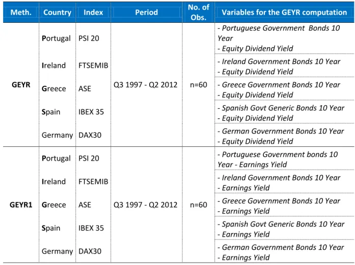
In this dissertation this ratio will be computed for 5 countries according to the information provided by 10 years government bonds and the representative indexes of each stock market per country:

Portugal – PSI 20 (Portuguese Stock Index)

Ireland – ISEQ (Irish Stock Exchange Quotien)

Greece – ASE (Athens Stock Exchange) Spain - IBEX 35 (Iberia Exchange)

Germany – DAX 30 (Deutscher Aktien-Index)

The GEYR is defined as a ratio that contemplates long-term government bond market yield and stock market yield. The bond and stock market yields are respectively approximated by the yield-to-maturity on long-term government bonds and by the equity yield of the most representative stock index. Equity markets concern to the obtained yield of companies listed in index, i.e. it is the yield from the index. In the GEYR computation, the stock market index of each country

(24)

15 allowed us to collect information about the dividend yield index and 10-year government bonds allowed us to withdraw information about the bond yield variable. This information was extracted from the representative indexes of each country through Bloomberg terminal. Notice that in this study, the GEYR is perceived as market analysis study, i.e. the goal is to see the market yield as a whole and not individualize it for each constituent company of the index. Therefore, every time we address implicit variables in the computation of the ratio, that’s a different approach referring to global market of stocks/ bonds concerning each country, according to the representative indexes previously described.

In the last few years it has been placed special attention to the GEYR development. Some researches concentrate their attention to a similar ratio, the so-called Fed-model, which weighs stock markets by comparing stock and bond yields. According to the Fed-model, the stock market earnings yield index should be compared to 10-year government bond yield (Vila Wetheritt and Weeken, 2002). When earnings yield index is superior to bond yield, stocks are considered cheap. On the other hand, if 10-year government bond yield exceeds earnings yield, stocks are considered expensive. The difference between the GEYR and the Fed-model is that in the GEYR framework researchers utilize dividends yield index and in the Fed-model they use earnings yield Index. As it is known, financial ratios are financial instruments of analysis that should be used individually. By presenting two kinds of ratios, it is also provided a comparison between them, increasing information range in order to enable value added on decision-making by analysts and so empowering investments efficiency. Therefore, in the first case, the GEYR takes the dividend yield index as input. In alternative it features the earnings yield (inverse of price-to-earnings ratio).

So, we will now present the general formula for the GEYR computation:

(25)

16

Bond Yield – 10-years Government Bond Yield for each country or coupon amount/ price bond

Dividend Yield Index – Dividend per “stock’s”/Price per “Stock’s” – in this case the “stock”

represent the “equity”, i.e. most representative stock index.

This is equivalent to:

Where: – Price of Bonds – Price of Equity – Coupon

– Dividend from equity

According to the Fed-model (GEYR1) the ratio will be:

Where:

Bond Yield – 10-years Government Bond Yield for each country or coupon amount/ price bond

Earnings Yield Index – Inverse of price-earnings ratio (1/ (P/E)) or EBIT/ Enterprise Value

The main goal of this ratio is to detect mispricing situations between equity markets and bonds markets, providing arbitrage opportunities between the two financial securities. To be able to detect these situations, it becomes important to know how to interpret the results that come from the ratio. According to Brooks (2001, p.11), “If the GEYR becomes high relative to its long-term level, equities markets are viewed as being expensive relative to bonds. The expectation then is that for given levels of bond yields, equity yields must increase which will occur through a fall in equity market prices. Similarly, if the GEYR is way below its long-term level, bonds are

(3) (2)

(26)

17 considered expensive relative to stocks, and by the same analysis, the price of the latter is expected to increase.” Thus, in its crudest form, an equity trading rule based on the GEYR would

say “If the GEYR is low, buy equities; if the GEYR is high, sell equities” (Brooks and Persand, 2001, p. 11).

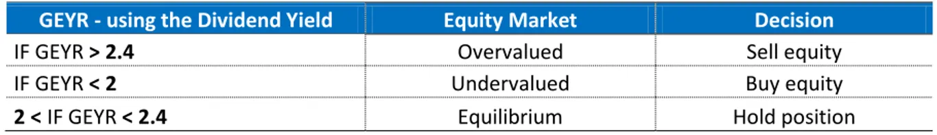
However, the corresponding level of a “low” or “high” value of the GEYR depends on the methodology that is being used. It all starts by analyzing the critical values of the first methodology of the GEYR (the one that contemplates dividend yield index). According to Hoare Govett3 (1991) the GEYR rule states that investors should buy equities if the GEYR < 2, sell equities and invest in gilts if the GEYR > 2.4. This means that if the value of the GEYR is superior to 2.4, then stocks are overvalued4 and consequently we should sell them and invest in bonds, in order to be able to relish the arbitrage strategy. On the other hand, if the GEYR value is inferior to 2, stocks are undervalued5, which means, a stock is valuing less than its book value. If the GEYR is between 2 and 2.4, the market is balanced and in these conditions it should sustain unchanged this position, because there is no possibility of arbitrage. Another ratio indicator that may provide us additional information about the market behavior is the payout ratio that is related to the results from the dividend yield index. Low payout ratio means that a company is mainly focused on retaining its earnings more than paying out dividends. This ratio also indicates how well earnings upkeep the dividend payments. The lower the ratio, the more secure is the dividend, since smaller dividends are easier to payout than larger dividends. We can affirm that generally a low payout, (usually inferior to 50%) tends to provide a higher value for the GEYR and if this value is superior to 2.4, ceteris paribus, consequently the best trading strategy will be to sell equities. On the contrary, a higher value for payout (generally superior to 50%), ceteris

paribus, tends to provide a lower value for the GEYR and if this value is inferior to 2, the best

strategy will be to buy equities.

Down below there is a Table 1 that demonstrates briefly the contents previously described.

3_{After conducted studies, he defined that critical values should be used as rule by the analysts.} 4

When stock price is superior to its intrinsic value.

(27)

18

Table 1: Strategy Decision with the GEYR results (using dividends yield index)

This table sums up trading strategies considering the critical values used on the first approach of the GEYR computation that uses dividend yields as denominators.

GEYR - using the Dividend Yield Equity Market Decision

IF GEYR > 2.4 Overvalued Sell equity

IF GEYR < 2 Undervalued Buy equity

2 < IF GEYR < 2.4 Equilibrium Hold position

Using the second methodology for the GEYR1 computation, in which the only difference is that earnings yield are considered on the formula’s denominator, the result analysis is slightly different. GEYR1 ratios greater than 1 imply that equity markets are overvalued, while numbers less than 1 mean they are undervalued, or that prevailing bond yields are not adequately pricing. If the GEYR1 is above normal levels the assumption is that the price of stocks will decrease thus lowering the GEYR1. When the GEYR1 value is equal to 1, we can affirm that it is better to hold position in the market and not buy or sell securities. So, the return to get bonds is higher than equity, if the GEYR1 has values superior to one, which means we must invest in bonds, i.e sell equity and buy bonds. This happens like this because, since stocks have prices above their intrinsic value, we are selling them for a superior value, obtaining an “earning”. On the other hand we should invest in bonds. On the opposite, if the value of earnings yield rises, it will cause a result on the GEYR1 inferior to 1. By then, we should buy equities and sell bonds and, we should buy stocks because their value is below their intrinsic value, so we spend less to obtain them. Down below there is a summary Table 2 that identifies arbitrage opportunities before the GEYR1 results.

Table 2: Strategy Decision with the GEYR1 results (using earnings yield)

This table sums up trading strategies considering the critical values used on the second approach of the GEYR computation that uses earning yields as denominators.

GEYR* – using Earnings Yield Equity Market Decision

IF GEYR1 > 1 Overvalued Sell equity

IF GEYR1 < 1 Undervalued Buy equity

(28)

19 According to Brooks (2001) the accuracy of this ratio varies from country to country and considering the agreed dividend distribution policy, the one that through the years has been suffering major alteration, there is no precise way to evaluate the results of this ratio. Moreover, the results of both ratios may not be in conformity. For instance, one can state that the best strategy will be sell equities and the other may state that the best strategy it to buy equities markets. In these cases, it is preferable to call on other indicators or financial ratios, in order to complement the analysis and comprehend the best market trend. In the empirical results chapter we will analyze the history of the ratio and understand which were predominant strategies in each country.

4.2. Pros and Cons of the GEYR

As in all financial ratios, this one also presents some pros and cons, since they have implicit variables that not always range in the same way, like the dividend distribution policy. The preference between high or low dividends ranges according not only to the company, but also to the surrounding political and economic environments where the company is inserted. The advantages of opting for low dividends go through the existence of personal taxes that generally favor capital gains to the detriment of the dividends and the cost of issuing new stocks. Buyback stocks has, like increasing the dividends value, a flag effect to the market and due to that, these indicators should be analyzed and pondered individually when a decision based on the GEYR is being made, so that afterwards a conclusion may be drawn. A company will opt for buyback stocks when it believes that equities are overvalued. Therefore, rather than just distribute equities to stockholders, the company will be investing, enabling the possibility of selling equities when their price is rising. Due to information asymmetry, the market faces buyback stocks by the company as a sign that they are undervalued and consequently the equities price raises, being another argument in favor of buyback stocks.

On the other hand, the inherent advantages of a high dividend distribution policy are due: to the information asymmetry, indicating that sometimes stockholders do not have access to the same

(29)

20 information that managers do; to the agency costs6 that reflect the conflicts inherent to the interests between stockholders and managers and still the fact of immediate income preference due to transaction costs. Transaction costs are well-reflected on the GEYR, so it is important that this “invisible” cost is always pondered by the analysts when analyzing the values from the ratio. More recently some analysts have been analyzing the power of the GEYR. According to John Higgins at Capital Economics7 “equities are real assets”. So at the very least “this suggests we ought to be comparing the dividend yield with the yield on index-linked gilts (which offer an inflation-linked return), rather than conventional gilts". There is also the problem that the dividend yield on stocks is influenced by the expected real (post-inflation) growth rate for equities. As a result, the difficulty with the GEYR is that we are not comparing equal terms. Gilt yields are nominal measures, i.e. inflation expectations affects them, whilst the dividend yield is a real measure, which means is not as affected. To get a glimpse of how this works, picture that long-term inflation expectations fall abruptly without affecting real economic growth, risk or real interest rates. There would be a fall in nominal gilt yields, but no alteration in the dividend yield. The GEYR would fall as well. However, it would be wrong to say that equities had abruptly become cheap, since – ex hypothesis – nothing has happened to them; real growth and the real discount rate applied to this growth haven’t changed. Consequently, the annual earnings yield on stocks (an annual earnings figure divided into the stock price) is perhaps a better guide to expected equity returns than dividend yields.

So it is important to present in this study the so-called Fed-model, in order to increase predictive power before the initial GEYR formula. This method was widely popularized in the US by the analysts, magazines and financial newspapers and it stated that the 10-year government bond yield should be contrariwise related to the expected earnings yield of the S&P500 index. In this model, the equity yield is proxied by the expected earnings yield. In practice, this model proposes asset allocation decisions based on the perceived degree of over and underpricing of the S&P500

6_{Debt agency costs: reflects a conflict of interests between stockholders and debt holders, i.e., the optimal decision}

for the stockholder may not be the optimal decision for the debt holder. Agency cost equity: conflict of interests between stockholders and managers. The manager who makes the decisions may be acting in his own best interest which may not be the stockholder’s best interest.

7_{John Higgins is Capital Economics’ Senior Markets Economist with 15 years of experience in financial markets as}

a trader, analyst and economist. Higgins identifies values in global asset markets based on our macroeconomic and policy projections. He contributes and edits our Capital Daily and he is responsible for producing regular updates and thematic pieces on key market developments.

(30)

21 concerning its fair value. Still, despite of the shaky theoretical foundations of the GEYR, proponents underline its strong relevance as an empirical description of stock prices (Lander, Orphanides and Douvogiannis, 1997; Asness, 2003; Campbell and Vuolteenaho, 2004). The clean ‘mechanical’ relationship implicit by the GEYR is attractive for instinctive reasons. Firstly, market participants persistently arbitrage the stock and bond markets, allocating financial resources between equities and long-term bonds by actively relating the corresponding bond and stock market yields. To be involved in such operation, market participants rely on the ‘substitution effect’ between stocks and bonds. Secondly, they take advantage of low interest rates in order to buy stocks on margin through ‘carry trade’ operations. Stock markets indirectly take advantage from a low-rate environment as portfolio managers incur low borrowing costs when they are buying stocks. These portfolio managers sell their stocks to hide their rising borrowing costs, when interest rates rise. Due to these reasons, there are many practitioners that view the GEYR as an augmented valuation ratio, which not only takes stock/ earning yields into account, but also compares them to bond yields.

(31)

22

5. Methodology

In this chapter we present and explain some concepts to better understand the application of cointegration tests. Section 5.1 refers to some basic concepts that are needed to the previous study of time series, like the case of stationarity/ nonstationarity distinction, as well as different approaches of data processing when we stand before nonstationary series (hypothesis that turn the series stationary). In section 5.2 we explain the Granger causality and this test is only applied to the stationary series, so its interpretation and analysis will be presented in this section. Lastly, in section 5.3 it will be presented inherent concepts to the cointegration study such as the Engle-Granger (two-step method) and the Johansen method. Also featured are some implicit methodologies in these methods, such as VAR, VECM and the Dickey-Fuller test.

5.1. Stationarity

When we work with econometric models and posteriorly apply cointegration tests, the first step is to check the series behavior and draw some conclusions on stationarity. A time series is composed of random variables{ } , therefore these sets of variables are sorted in time, therefore we have a stochastic process8. There are two types of stationary: the strictly stationary and weakly stationary. A strictly stationary process i for any

Where F represents the joint distribution function of the random variables’ set. It can also be stated that the probability measure for the sequence { } is the same for{ } . A strictly stationary series tells us that there are no changes in the series over time. Its behavior is always constant and there are no structural breaks, i.e. the distribution of its values remains the same as

8_{Family of random variables indexed by t elements that belong to a certain timeslot. Intuitively, if a random variable}

is a real number that ranges randomly, a stochastic process is a temporal function that ranges randomly, in a simplified way and so we can say that stochastic processes are randomly processes that depend on time.

(32)

23 time passes by, implying that the probability that falls within a particular interval is the same as now as it is at any time in the past or in the future.

The weakly stationary is more usual and better to analyze financial and economic series. This concept consists in:

Mean: Variance: ;

Autocovariance:

The unknown parameters are , , and they change with t. Therefore, the statistical proprieties of the stationary concept of a time series do not change over time, i.e. a stationary series has, as it was previously presented a constant mean, a constant variance and a covariance between lagged values of the series depend only on the lag, in other words, the temporal “distance” between them (Gujarati (2005)). Simultaneously, nonstationary series may be detected by their mean, since in a nonstationary series it ranges over time, consequently the series will show several types of tendencies, thereby not obeying to the stationary rules. To estimate a “good” model is not enough the confirm the stationarity of a series, we have to analyze its residues, i.e. a process in which its mistakes present zero mean, constant variance and no serial correlation and that is called white noise9:

When we stand before the white noise process, we can conclude that the series is stationary. Understanding white noise is tremendously important for at least two different reasons: First, processes with such richer dynamics are built up by taking simple transformations of white noise. Second, one-step-ahead forecast errors from good models should be white noise. After all, if such forecast errors are not white noise, then they are serially correlated, which means that they are

9_{WN implies stationary, but a series can be stationary and not be WN.}

(5) (6) (7) (9) (10) (8)

(33)

24 forecast, and if forecast errors are forecast, then the forecast cannot be very good. Thus it is important that we understand and be able to recognize white noise.

As it is obvious, in the financial and economic world, the majority of the series are nonstationary, due to the existence of structural breaks that provoke unexpected alterations. In other words, the common characteristic between nonstationary series is that they have a increasing tendency over time, making their mean non-constant. When we have a stationary series, shocks tend to gradually disappear. This means that a shock at time t will have a small effect in period t +1, a smaller effect in time t +2 and so on. This situation is not the same as in the case of nonstationary data, where the persistence of shocks will always be infinite, so that for a nonstationary series, the effect of a shock during time t will not have a smaller effect in time t +1 and in time t +2 and so on. Therefore, it is important to develop methods and models that can study nonstationary series behavior and consequently obtain a good predictive model. The development of the cointegration concept becomes thereby important, since it’s one of the technics applied to the nonstationary series with the objective of checking the existence of any long-term equilibrium relationship between them. Having said this, here are two very distinct models that allow nonstationary series transformations. The model (or process) in trend stationary (TSP – Trend Stationary Process) and by differentiation of stationarity (DSP – Difference Stationary Process) or unit root.

According to the hypothesis TSP the series is:

Where is a time fuction and represents a stationary process. For example, assuming a linear deterministic trend, the most ordinary hypothesis, we’d have:

However, because economic series generally have a growth tax approximately constant, the exponential trend model reveals itself frequently more accurate:

(11) (12) (13) (14)

(34)

25 Nevertheless, in this model, deviations from the trend are white noise, i.e. are stationary. Although the persistence of structural breaks on economic series makes us conclude that not always deviations from the trend are stationary. In these cases, the best way would be to use the DPS (Difference Stationary Process) model. Imagining, e.g., a random walk with drift10:

In this case we can easily verify the presence of a increasing tendency (since ). The major difference of this model comparing to the TSP model is that this one introduces a stochastic trend. In other words, deviations from the deterministic trend, according to the DSP or unit root hypothesis, are nonstationary. If the series is differentiated d times before becoming stationary, then it contains d unit roots and we say it is integrated of order d, denoted by . Box Jenkins (1944) and more recently Nelson and Plosser (1982) argue that not all nonstationary series can be converted into stationary series by differentiation, however there is strong evidence that most of the economic and financial series tend to be differentiated of order 1, denoted by I(1). If we have more than one series under study, all of them have to be stationary with the same order of integration so that we can apply cointegration tests. Cointegration tests will be applied to the series in level (Gujarati, 2000 and Terrence, 2003). The denotation for a stationary series is I (0). In order to verify if the series was sufficiently differentiated to become stationary, there are the unit root tests. Hypothesis to test are the following:

(unit root test)

Consider the easiest example and tested through OLS the model AR (1):

In this case, the test statistic will be:

10_{Random Walk concept: taking several consecutive steps, each in a random direction. The direction of a point on}

the way to the next is chosen randomly and no direction is more likely than another. If the series that is being fitted by a random walk model has an average upward (or downward) trend, it is expected to continue likewise in the future. We should include a non-zero constant term in the model i.e., assume that the random walk undergoes "drift”.

(15)

(35)

26

H₀: ρ = 1

H_a: ρ ≠ 1.

Equation 16 may be rewritten as:

Making we have:

In this case, we are testing:

H₀:

H_a:

We can conclude that we stand before a model in which there is no serial correlation of errors, therefore if we effectively do not reject H_{0 ,}_{it means that} i.e. we stand before a random walk11 series. Because is white noise, it is stationary, which means the first differences of a random walk temporal series are stationary.

It is important to reference that Dickey and Fuller show that, under the null hypothesis in which , the estimated t value of the coefficient follows a τ (tau) statistic. These authors calculated critical values of the tau statistics based on Monte Carlo simulations. MacKinnon prepared more extended tables that nowadays are incorporated in several econometric software. In specialized literature, tau statistics or tau test τ is known as the Dickey-Fuller (DF) test, in order to honor its founders. It is interesting to notice that when the hypothesis is rejected (i.e. the temporal series is stationary) we can use the usual t Student test. This Dickey-Fuller test can be applied to the following models:

Where t is a time variable or tendency.

11

Random Walk concept: taking several consecutive steps, each one in a random direction. The direction of a point on the way to the next is chosen randomly and no direction is more likely than another.

(17)

(18)

(19) (20) (21)