Performance-based design of bolted steel structures

(1)

Dissertation

Master in Civil Engineering – Building Construction

Performance-based design of bolted steel structures

Hernán Alberto Coloma Peralta

(2)

(3)

Dissertation

Master in Civil Engineering – Building Construction

Performance-based design of bolted steel structures

Hernán Alberto Coloma Peralta

Dissertation developed under the supervision of professor Hugo Filipe Pinheiro Rodrigues, adjunct professor at the School of Technology and Management of the Polytechnic Institute of Leiria.and professor Byron Armando Guaygua Quillupangui at Central University of Ecuador

(4)

(5)

1. Dedication.

This work is dedicated to my family, girlfriend, and friends that has been my major inspiration in my life their support and love have guide me to this journey giving me the force to continue and overcome all prove that I have faced.

(6)

ii

2. Thanks.

I would like to thanks the IPL’s teachers for shearing their knowledge and support during the master and I want to thanks specially to my advisor Professor Hugo Filipe Pinheiro Rodrigues for his friendship, guide and advice that make possible this thesis.

I would like to thanks engineer Alex Farinango and Sedemi company for provide the information and characteristic of the study case.

I would like to thanks to the Universidad Central del Ecuador and SENESCYT for the given opportunity.

Finally, I would like to thanks to the most important people in my life my family, girlfriend and friends. During the develop of this thesis, they encourage me to give my maximum effort.

(7)

iii

3. Abstract

In the last decade, the philosophy of seismic design has change from the force-based design to performances based design due to the advantage that presents. Also, the performance based the design presents less simplification of the force method representing in a more accurate form the real behavior of the structure. One method of this new philosophy is the direct displacement-based design (DDBD); this method permits to take in count in more exact form the nonlinear behavior than the force method. The DDBD can be used to design new structures and analyze the retrofit of structures of concrete, steel, composed and timber. In the case of steel structure, the formulas used represent a bilinear behavior of the material and the yield displacement proper of the steel structural system. This displacement method can be used with deferent demands optimizing the design.

Another technique used in the performed based design is the pushover analysis. This method can be used to design new structures, evaluated design, optimizing design and retrofit the structures. The pushover considers in a more accurate form the nonlinear behavior of the structure, and it show the fail mechanism; it can analysis if the structure presents the condition of strong column weak beam. Also, it can be determining the ductility and the damping of the structure.

Another concert that engineers have nowadays is the design higher structures that satisfy high demands. In order to reaches the performance that require this demand seismic protection systems are used such as damper and insulators. In this project, the fluid viscous dampers are study; the advantages that present their used and the behavior faced a seismic event using time history analysis.

Finally, it is designing a Fluid viscous dampers in study case to analysis the performance achieved and the advantage presented in the structure.

Keywords:

 Performance-based of in steel structures

 Direct displacement-based design steel frame structures.

 Pushover steel frame structures.

(8)

iv

4. List of figures

Figure 1. a) Equivalent structure b) Secant or effective stiffness. ... 4

Figure 2. a) Equivalent D Plan location dampers first iteration study case amping vs. Ductility b) Design Displacement Spectra. ... 5

Figure 3. Elevation and plan view. Source: author ... 7

Figure 4. Elastic acceleration spectra according NEC 15 ... 9

Figure 5. Elastoplastic and bilinear inelastic behavior model. ... 12

Figure 6. Acceleration spectrum according NEC 15 ... 14

Figure 7. Displacement spectrum according NEC 15 ... 14

Figure 8. Maximum drift in force design ... 19

Figure 9. Maximum drift in displacement design ... 19

Figure 10. Longitudinal section of fluid viscous damper ... 24

Figure 11. Force-velocity relationship FVDs ... 24

Figure 12. Force displacement relationship ... 25

Figure 13. Hysteretic curve ... 25

Figure 14. FVDs efficiency by their configuration. ... 26

Figure 15. Artificial accelerogram 1. ... 30

Figure 18. Matching accelerogram 1 with response spectra ... 31

Figure 21. Location of FVDs Y direction. ... 36

Figure 22. Location of FVDs X direction. ... 37

Figure 23. 3D view of Location of FVDs. ... 37

Figure 24. Energy in the structure without dampers. ... 43

Figure 25. Energy in the structure without nonlinear dampers. ... 43

Figure 26. Energy in the structure without lineal dampers. ... 44

Figure 27. Nonlinear behavior of the structure without dampers. ... 45

Figure 28. Nonlinear behavior of the structure without nonlinear dampers. ... 45

Figure 29. Nonlinear behavior of the structure without linear dampers. ... 46

(9)

v

Figure 31. Pushover procedure. ... 50

Figure 32. Plastic hinge behavior ... 50

Figure 33. Story forces based in triangular and first mode distribution... 53

Figure 34. Bolted flange plate moment connection. Source: AISC 358-10 ... 54

Figure 35. Plastic hinge location in frame. ... 55

Figure 36. Capacity curve direction x ... 58

Figure 37. Capacity curve direction X DBDD design ... 57

Figure 38. Capacity curve direction X Forces design. ... 57

Figure 39. Capacity curve direction Y ... 58

Figure 40. Capacity curve direction Y DBDD design ... 59

Figure 41. Capacity curve direction Y DBDD design ... 59

Figure 42. Architectonical 3D view study case. ... 61

Figure 43. Architectonical plant residential use study case. ... 62

Figure 44. Architectonical plant parking use study case... 62

Figure 45. 3D view study case. ... 62

Figure 46. Structural plan view study case. ... 63

Figure 47. Structural element sections study case. ... 63

Figure 48. Design acceleration spectra. ... 64

Figure 49. Triangular, first mode, Uniform and SRSS lateral load pattern. ... 646

Figure 50. Beam plastic hinge location in plan. ... 64

Figure 51.Columns plastic hinge location in plan. ... 69

Figure 52. Layered model of shear walls. ... 69

Figure 53.Plastic hinges develop in X direction. ... 71

Figure 54. Capacity curve in X direction. ... 71

Figure 55. Performance point study case X direction. ... 715

Figure 56. Structure performance by VISON 2000. ... 715

Figure 57. Plastic hinges develop in Y direction. ... 75

Figure 58. Capacity curve in Y direction. ... 75

Figure 61. Plastic hinges develop in X direction. ... 79

Figure 62. Capacity curve in X direction. ... 79

Figure 63. Figure 62. Capacity curve in X direction... 83

(10)

vi

Figure 65. Plastic hinges develop in Y direction. ... 83

Figure 67. Performance point study case Y direction ... 87

Figure 69. Artificial accelerogram 1 of the study case. ... 87

Figure 72. Matching accelerogram 1 with response spectra study case. ... 88

Figure 76. Elevation view B axis of dampers in X direction study case. ... 95

Figure 77. Elevation view D axis of dampers in X direction study case. ... 96

Figure 78. Elevation view 3 and 5 axes of dampers in X direction study case. ... 96

Figure 79. Elevation view 8 and 10 axes of dampers in X direction study case.. ... 96

Figure 80. Energy in the structure without dampers study case. ... 101

Figure 81. Energy in the structure without linear dampers study case. ... 100

Figure 82. Nonlinear behavior of the structure without dampers. ... 100

Figure 83. Plastic hinge performance without dampers. ... 102

Figure 84. Nonlinear behavior of the structure without linear dampers. ... 102

Figure 85. Plastic hinge performance according with dampers. ... 103

Figure 86. Hysteresis behavior THSISMO3B. ... 103

Figure 87. Plan location dampers first iteration study case ... 103

Figure 88. Elevation location and configuration of the dampers first iteration ... 1056

(11)

vii

5. List of tables

Table 1. Steel mechanical properties. ... 7

Table 2. Dead load description... 8

Table 3. Live load description ... 8

Table 4. Self-weight. ... 10

Table 5. Seismic or reactive mass. ... 10

Table 6. Parameters for the calculation of DDBD substitute structure ...¡Error! Marcador no definido. Table 7. Shear distribution. ... 16

Table 8. Shear distribution. ... 16

Table 9. Increased lateral floor by P-Δ effect ... 18

Table 10. Overturning by P-Δ effect ... 18

Table 11. Final element sections. ... 20

Table 12. Total weight for force and displacement design ... 20

Table 13. Comparison of lateral forces between methods. ... 21

Table 14 Values of λ parameter. ... 29

Table 15. Maximum and minimum drifts X direction. ... 32

Table 16. Absolute maximum drifts X direction. ... 33

Table 17. Maximum and minimum drifts Y direction ... 33

Table 18. Absolute maximum drifts Y direction. ... 33

Table 19. Parameters for FVD damping coefficients Y direction ... 33

Table 20. Parameters for FVD damping coefficients X direction ... 36

Table 21. Maximum and minimum drifts X direction with dampers. ... 368

Table 22. Absolute maximum drifts X direction with dampers ... 38

Table 23. Maximum and minimum drifts Y direction with dampers ... 38

Table 24. Absolute maximum drifts Y direction with dampers. ... 39

Table 25. Parameters for FVD damping coefficients Y direction. ... 39

Table 26. Parameters for FVD damping coefficients X direction ... 40

Table 27. Maximum and minimum drifts X direction with lineal dampers ... 41

Table 28. Absolute maximum drifts X direction with lineal dampers ... 41

(12)

viii

Table 30. Absolute maximum drifts X direction with lineal dampers... 42

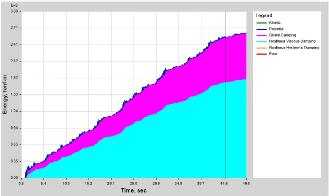
Table 31. Energy dissipation of the structure for TH1,1 at 45 seconds for structure with and without dampers. ... 44

Table 32. Axial damper forces for TH1,1 ... 47

Table 33. Non-lineal gravitational load ... 51

Table 34. Modal Participating Mass Ratios ... 52

Table 35. Story forces based in triangular and first mode distribution. ... 52

Table 36. Capacity curve DBDD and force design X direction ... 56

Table 37. Capacity curve DBDD and force design Y direction ... 58

Table 38. Result parameters from Pushover X direction ... 60

Table 39. Result parameters from Pushover Y direction ... 60

Table 40. Study case live load ... 65

Table 41. Total dead load in story floors ... 65

Table 42. Total dead load in communal areas. ... 65

Table 43. Total dead load in parking. ... 65

Table 44. Modal mass participation study case. ... 67

Table 45. SRSS lateral load for the X and Y direction ... 67

Table 46. Capacity curve data and plastic hinge develop X direction ... 72

Table 47. Performance point study case X direction ... 74

Table 48. Capacity curve data and plastic hinge develop Y direction. ... 76

Table 50. Capacity curve data and plastic hinge develop X direction ... 80

Table 51. Performance point study case X direction. ... 82

Table 52. Capacity curve data and plastic hinge develop Y direction. ... 84

Table 54. Maximum and minimum drifts X direction of the study case. ... 89

Table 55. Absolute maximum drifts X direction study case. ... 90

Table 56. Maximum and minimum drifts Y direction of the study case ... 90

Table 57. Absolute maximum drifts Y direction study case ... 90

Table 58. Parameters necessaries to compute the FVD damping coefficients Y direction study case ... 93

Table 59. Parameters necessaries to compute the FVD damping coefficients X direction study case ... 94

(13)

ix

Table 61. Absolute maximum drifts Y direction with lineal dampers study casez.... 98

Table 62. Maximum and minimum drifts X direction with lineal dampers used study case ... 99

Table 63. Absolute maximum drifts X direction with lineal dampers study case ... 99

Table 64. Energy dissipation of the structure for THSISMO3,4 at 28,94 seconds for structure with and without dampers study case... 101

Table 65. Linear damper force study case for THSISMO3B ... 104

Table 66. First iteration result for THSISMO 3A Y THSISMO 3B. ... 106

(14)

x

6. Lista de siglas

 Δi = Floor displacements at level i

 δi = Normalized inelastic mode of level i

 δc = Critical distortion

 Hi = Height of level i

 Hn = Height of roof level

 DL = Dead Load

 LL =Live Load

 W = Reactive mass

 b section width

 bw width of web of flanged beam

 C constant

 Cm centre of mass

 E modulus of elasticity

 E force induced by seismic action

 Es steel modulus of elasticity

 Fsec secant modulus of elasticity of confined concrete at peak strength

 F force

 fd damping force

 Fel seismic force corresponding to elastic spectrum

 Fm maximum force

 ft tension strength

 fyh yield strength of hoop or spiral transverse reinforcement

 fyo maximum feasible steel strength

 fu steel ultimate stress

 G shear modulus; gravity load

 g acceleration due to gravity, 9.805m/s

 H height

 He effective height of SDOF approximation to multi-storey building

 Ht height of mass / in building design

 Hs storey height

 h section depth

 hb beam section depth

 hc column section depth

 I importance factor in force-based design; section moment of inertia

 I multiplier applied to design seismic intensity level

 It moment of inertia of beam section

 lc moment of inertia of column section

 K structure stiffness

 ka assessed structure stiffness at limit state

 Ke structure effective stiffness for DDBD

 Ki initial (elastic) stiffness

 k lr lateral stiffness of lead-rubber bearing

 Ks structure secant stiffness

(15)

xi

 Lb beam length

 Lc distance from critical section to contraflexure point

 LP plastic hinge length

 m mass

 me effective mass participating in the fundamental mode

 n number of storeys in multi-storey building

 OTM overturning moment

 PGA peak ground acceleration

 R force-reduction factor applied to elastic spectrum in force-based design

 reduction factor applied to displacement spectrum for damping

 force-reduction factor related to ductility

 Sa(T) period-dependent response acceleration coefficient from response spectrum

 T period

 T seismic tension force in column of frame

 tb period at end of maximum spectral response acceleration plateau

 Tc corner period in displacement response spectrum

 Te effective period for DDBD

 V shear force; shear strength

 Vc column shear force

(16)

(17)

C

ontent table

1. DEDICATION. ... I 2. THANKS. ... II 3. ABSTRACT ... III 4. LIST OF FIGURES ... IV 5. LIST OF TABLES ... VII 6. LISTA DE SIGLAS ... X

1. PERFORMANCE-BASED DESIGN ... 1

INTRODUCTION ... 1

MOTIVATION AND OBJECTIVES. ... 2

ORGANIZATION OF THE THESIS... 3

... 3

2. DIRECT DISPLACEMENT BASED DESIGN (DDBD) ... 4

DIRECT DISPLACEMENT BASED DESIGN (DDBD) ... 4

APPLICATION OF THE DBDD THEORY ... 6

2.2.1. Structure geometry ... 6

2.2.2. Structure mechanical and seismic characteristics ... 7

2.2.3. DBDD analysis. ... 9

2.2.3.1. Property calculations of equivalent single degree of freedom system ... 9

2.2.3.2. Floor lateral forces and base overturning moment calculation. ... 15

2.2.3.3. P-Δ Effect ... 17

COMPARISON OF RESULTS OBTAINED FROM DBDD WITH FBD. ... 18

2.3.1. Quantity of steel obtained. ... 20

2.3.2. Base shear and lateral forces. ... 21

3. FLUID VISCOUS DAMPER ... 22

INTRODUCTION ... 22

FLUID VISCOUS DAMPERS ... 23

3.2.1. Fluid viscous dampers parts and working. ... 23

3.2.2. Fluid viscous dampers configuration and location. ... 26

3.2.3. Procedures for the design of the FVDs ... 27

3.2.4. Fast Nonlinear Analysis (FNA) ... 27

3.2.5. Constants and coefficients determination of FVDs... 28

(18)

2

3.3.1. Non-lineal time history analysis without dampers. ... 30

3.3.2. Determination of FVDs parameters. ... 34

3.3.3. Nonlinear Viscous Dampers Parameters ... 35

3.3.4. Results nonlinear Viscous Dampers ... 37

3.3.5. Linear Viscous Dampers Parameters ... 39

3.3.6. Results linear Viscous Dampers ... 41

3.3.7. Input seismic energy in the structure. ... 42

3.3.8. Inelastic behavior of the structure. ... 44

3.3.9. Dampers forces and behavior. ... 46

4. STATIC NONLINEAR ANALYSIS (PUSHOVER) ... 49

INTRODUCTION ... 49

PUSHOVER APPLICATION ... 51

4.2.1. Pushover gravitational load ... 51

4.2.2. Pushover lateral load patterns ... 51

4.2.3. Plastic hinge location ... 54

4.2.4. Pushover results. ... 55

5. STUDY CASE ... 61

STUDY DESCRIPTION. ... 61

5.1.1. Gravitational loads. ... 65

PUSHOVER STRUCTURE WITH SHEAR WALLS ... 66

5.2.1. Lateral Load Patterns ... 66

5.2.2. Non-lineal behavior of the structural elements. ... 68

5.2.3. Beam. ... 68

5.2.4. Columns. ... 68

5.2.5. Shear walls ... 69

5.2.6. Applied loads. ... 70

5.2.7. Non-lineal gravitational load. ... 70

5.2.8. Push X. ... 70

5.2.9. Push Y. ... 70

5.2.10. Result pushover X direction. ... 71

5.2.11. Capacity curve and plastic hinge develop. ... 71

5.2.12. Performance point. ... 73

5.2.13. Result pushover Y direction. ... 75

5.2.14. Capacity curve and plastic hinge develop. ... 75

PUSHOVER STRUCTURE WITHOUT SHEAR WALLS ... 79

(19)

3

5.3.2. Capacity curve and plastic hinge develop... 79

5.3.4. Result pushover Y direction. ... 83

5.3.5. Capacity curve and plastic hinge develop... 83

FVDS IMPLEMENTATION ... 87

5.4.1. Non-lineal time history analysis without dampers. ... 87

5.4.2. Linear Viscous Dampers Parameters ... 91

5.4.3. Results linear Viscous Dampers ... 97

5.4.4. Input seismic energy in the structure. ... 100

5.4.5. Inelastic behavior of the structure. ... 101

6. CONCLUSIONS ... 108 CONCLUSIONS OF CHAPTER 2. ... 108 CONCLUSIONS OF CHAPTER 3. ... 108 CONCLUSIONS OF CHAPTER 4. ... 109 CONCLUSIONS OF CHAPTER 5. ... 110 7. BIBLIOGRAPHY ... 112 8. ANNEX ... 114

(20)

(21)

1

1. Introduction

Introduction

The force-based design has been the most used method for the seismic design of structures in which the structure is designed for equivalents static forces due to the action seismic event. In order to get the equivalent forces, the period of the structure is assumed based in the structural system, material, and height of the building. Using the calculated period, the based shear is obtaining from an acceleration design spectrum that takes in account the characteristics of the foundation soil, importance of the structure, irregularities and an assumed inelastic behavior by using a factor (behavior factor “q” in Europe or response reduction factor “R”). The based shear is distributed as a lateral load acting in each floor, and the distribution is according a modal analysis.

A control in this method is the inelastic inter-story drifts limited by a country code; if the drift is exceeding the limited, the stiffened and strength of the structural elements must be increased. The problems presented in this method are the assumptions made such as the constant stiffens, ductility based in the structural system used instead of the characteristics of the structure, simply inelastic behavior consider, and calculation of the structure period with empirical equation. These assumptions and simplification can lead to results that are far away of the real behavior of the structure.

In the last decades, researches and engineers have proposed and implemented seismic analysis methods based in displacement instead of acceleration overcoming the problems presented in the force method. The displacement method is based in the performance of the structure facing a demand. In this method, the ductility and period are computed based in the characteristic of the structure. Also, the structure can be designed to have different performances to different levels of hazards (Ghorbanie-Asl, 2007).

The performance is an indicator of the damage level that will occur after the seismic event in the building in structural and nonstructural elements. The performances are achieved with target displacements; the minimum performance is the life safety for residential structures for and operational building for special structures.

(22)

2

Motivation and objectives.

In the last decade, earthquakes with great magnitude has occurred in different countries killing, and injuring thousands of people for example (Vega, 2015):

 19/09/2017 Mexico (7.1 magnitude) killing 369 people.

 24/08/2016 Italy (6.2 magnitude) killing 300 people.

 16/04/2016 Ecuador (7.8 magnitude) killing 650 people.

 25/04/2015 Nepal (7.8 magnitude) killing around 9000 people.

The most common method useed to design structures is based in forces; this method has present deficiencies exposed in these earthquake. The more notable problems with the forces design are the use of factors to consider the ductility, over-strength and plastic behavior of the structure. Nowadays, the designers have to face larger and taller structures than building in the past; also, many structures have to accomplished new requirements such as zero dame in non-structural elements. These factors indicated the necessity of design methods that characterize in more realistic way the behavior of the structure. The performance-based design is a more realist approach. The Direct Displacement-Based Design (DDBD) and pushover are methods in this approached. Also, in order to get a better performance of the structures damping and isolations systems are used; this system can be used in new structure and rehabilitation. The DDBD and pushover are going to be analysis as method of the performance-based design in this thesis. Also, it is going to be use the fluid viscous damper to improve the performance of the structures.

The objectives of the thesis are

 To exhibit the advantages of the seismic design based on displacements over the force design in steel structure frames.

 To determine the performance of a structure designed by displacements and designed by force obtaining the ductile, capacity curve, performance point and plastic behavior in both cases.

 To increase the performance of a structure establishing the influence in the plastic behavior with the implementation of the fluid viscous dampers in a steel frame structure.

(23)

3

 To define the performance in a study case and implement fluid viscous instead of shear walls reaching a target drift.

 To verify the non-linear behavior of the study case with shear walls and with FVDs instead of the shear walls using a non-linear dynamic analysis (time history analysis)

Organization of the thesis

This work is divided in six chapters in the next paragraph is explained the content of each chapter in a summary way.

 Chapter one describes of the performance-based design. Motivation of the theme of the thesis and the objectives of it.

 Chapter two presents the theory of the Direct Displacement-Based Design and parameters necessary for this method. It is designed a regular steel frame structure (special moment frame) by the displacement and force method comparing the obtained results

 Chapter three implements of the fluid viscous dampers (FVDs) reaching a target drift. Theory and parameters necessary to compute the damping coefficients of the dampers are exposed, and it is explained the nonlinear dynamic analysis (Fast nonlinear analysis FNA) based.

 Chapter four performances a nonlinear static analysis (pushover) in the model’s design by displacements and forces with different lateral load patterns. Obtaining the ductile, capacity curve, performance point and plastic behavior in both cases.

 Chapter five is the study case in which is performed an analysis pushover including the effects of the high modes. A nonlinear dynamic analysis (FNA) will be done on the study case removing the shear walls obtaining the maximum drift then it will be incorporate the FVDs to reach the objective target. Another nonlinear dynamic analysis will be done in the structure with the dampers obtaining the performance of the structure.

(24)

4

2. Direct Displacement Based Design (DDBD)

Direct Displacement Based Design (DDBD)

In the decade of 1992 to 1994, Nigel Priestley, Mervyn Kowalsky and Bob Park developed an innovative seismic analysis method based in displacement focused in the performance of the structure (Priestley, Calvi, & Kowalsky,, 2007); nowadays, this method is known as Performance-based design). The Direct Displacement Based Design (DDBD) is a performance-based seismic design method where a structure of multi degree of freedom of liberty (MDOF) is analysis as an equivalent structure of simple degree of freedom (SDOF), and it is carried to a target displacement; the equivalent structure has an effective mass (me) and effective height (he) based in the original mass and height of the structure.

The SDOF has an effective stiffness equal of the secant stiffness (ke) of the bilinear stiffness model of the structure that takes in count the inelastic behavior of the structure.

The bilinear model is composed of the initial stiffness (ki) of the elastic behavior and the decreasing of the stiffness equal to the initial stiffness affected multiply by a coefficient. In the case of the DBDD, the effective stiffness is of a single degree of freedom.

Figure 1. a) Equivalent structure b) Secant or effective stiffness. Source: Timothy Sullivan; Progettazione basata sugli spostamenti per le Costruzioni in Acciaio: stato dell’arte

The equivalent damping (ξeq) has to provide a mechanism capable to dissipate the energy taking in count the lineal behavior (5% elastic damping) and nonlinear behavior (hysteretic damping); the computation of the ξeq considers the material, structural system and

(25)

5 the displacement ductility (μ); similarly, the equivalent damping is related to the structures ductility. After it is obtained the equivalent damping, a damping reduction factor is determined to obtain the displacement spectra corresponding to the calculated equivalent damping. (KARIMZADA, 2015)

Figure 2. a) Equivalent Damping vs. Ductility b) Design Displacement Spectra. Source. (KARIMZADA, 2015)

Form the target displacement (Δd), a line parallel to the x axel is draw until it intersects the displacement spectra corresponding to the equivalent damping finding the structure effective period (Teff) like in Figure 2; the effective stiffness can be calculated with effective period (Teff).

Knowing the effective period (Teff) and the target displacement (Δd), the base shear (VB) is determined; the found base shear is distributed in each floor according to the height and mass of the floor. In order to consider the effects of the contribution of the highest modes, the force assigned to the last floor is equal to the ten percent of the base share. Also, the DBDD can consider the effects of torsion, P-Delta, high modes, and irregularities by affecting the effects with a coefficient or applying modified formulas in the process.

Finally, the structure is design with the different combinations that involves the gravitational, wind, earth pressure and seismic load ensuring an adequate design of the building.

(26)

6

Application of the DBDD theory

The theory of the DBDD will be applied to a regular structure in plane and height, with a fixed foundation, and bolted connection (rigid connection – moment resistant connection). The predesign of the structure was according the AISC 360-16, AISC 358-16 and AISC 341-16; the sections of the structures are classified as high ductility sections according the AISC 341 (AISC Seismic Provisions for Structural Steel Buildings). The seismic parameters such acceleration spectra and displacement spectra were obtaining from the Ecuadorian Construction Code “NEC - SE – DS” (Norma Ecuatoriana de la Contruccion); likewise, the live load, dead load, load combination, and factors were taken from the NEC - SE – CG. The Ecuador.

2.2.1. Structure geometry

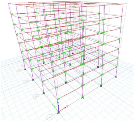
The structure has a floor area of 21x21m (441m2_{) divided in three bays of seven} meter in direction of X axel and Y axel; the total height of structure is a seven-floor building with 21.5m2_{of total height in which the first floor has 3.5 meters, and the other floors have} 2 meters of height.

The structural elements are hot rolled steel sections that accomplish the requirements of high ductility for seismic actions exposed in the Eurocode and American standards (AISC and ASCE).

Structural elements type of the predesign: Master beam VM1: W450X43 (450X120X8X10) Master beam VM1: W350X30 (350X100X6X8) Principal beams VP: W430X48 (430X140X8X10 Secondary beams: W200X14 (200X80X4X8) Columns: HSS 460X460X25

(27)

7

Figure 3. Elevation and plan view. Source: author

2.2.2. Structure mechanical and seismic

characteristics

Structure type: Special moment frame (AISC 341-16).

Column – Beam connection: Bolted Flange Plate (BFP) Moment Connection. Material: Steel A-36.

Table 1.

Steel mechanical properties.

Type of steel: A36

Fy = 36 Ksi 248 Mpa 25310357 Kg/m2 E = 29000 Ksi 199948 Mpa 20388898630 Kg/m2

(28)

8

Beam type: W (Profile I)

Column type: HSS (Tubular profile) Load applied according NEC15:

 Dead load

Table 2.

Dead load description.

Steel deck. Thickness=0.65mm and Height=55mm 7 Kg/m2 Filling concrete thickness of the steel deck 200 Kg/m2

Floor finishing. 30 Kg/m2

Walls 150 Kg/m2

Ceiling 13 Kg/m2

∑DL= 400 Kg/m2

Table 3.

Live load description.

Department 200 Kg/m2

200 Kg/m2

Seismic parameter:

 Location: Quito (Highlands)

 Seismic zone: V

 Factor according the site of implantation of the structure: Z=0.4; η=2.48

 Characterization of seismic hazard: High

 Soil type: C; r =1

Fa=1,20 Fd=1,11 Fs=1,11

 Structure importance: Residential I=1

 Plan and elevation factor: ΦP = ΦE=1

(29)

9

Figure 4. Elastic acceleration spectra according NEC 15 Source: Norma Ecuatoriana de la construccion

2.2.3. DBDD analysis.

2.2.3.1. Property calculations of equivalent single degree

of freedom system

 Design displacement of the substitute structure.

The design displacement (Δd) if the SDOF is computed according the mass distribution, height of each floor, inelastic mode shape, and critical displacement or drift. The critical displacement must be taken based in the ductility of the structural elements, desire performance to achieve, and the maximum drift specify in the local building code; in this case, the critical displacement was calculated with the maximum drift stipulated in the NEC-SE–DS.

The design displacement depends of the displacement shape of the real structure; the displacement shape considers the plastic behavior due to the formation of the plastic hinges and plasticization of the steel fibers in the first mode (Chopra & Goel, 2001)

(30)

10

Seismic or reactive mass calculation: The seismic mass considers that the totally of the

dead load and twenty-five percent of the live load. The analysis will be performed in the frame of the axes three.

𝑊 = 𝐷𝐿 + 0.25𝐿𝐿 Equation 1. (Reactive mass)

Table 4. Self-weight. Element Weight (Kg/m) Length (m) Weight (Kg) VM1 43 84 3612 VM2 30 63 1890 VP1 48 84 4032 VS 14 189 2646 C1 343 48 16485 Table 5.

Seismic or reactive mass

Distance X (m) Distance Y (m) Plant area (m2₎ Dead load ( Kg/m2₎ Live load ( Kg/m2₎ Self-weight (Kg) Reactive mass ( Kg/m2₎ Reactive mass (Kg) 21 7 147 480 200 33946 530 111856,2

 Critical displacement and inelastic mode shape.

The critical displacement based in the local code (NEC) due to the high ductility of the steel profile allows strains or deformations bigger than the maximum drift of the NEC; the maximum drift according to the NEC is 0.02 for force based designed and 0.025 for direct based displacement design that cover the performance level of life safety found in the FEMA 356.

The equations developed in 2006 by the professor Priestley, Calvi and Kowalsky were used to determine the inelastic mode shape. The floor displacement is proportional to the distortion of the analyzed floor, critical displacement, and inverse to the critical distortion; the critical distortion is the maximum distortion that in the majorities of cases is the distortion of the first floor.

(31)

11

Δ𝑐 = max 𝑑𝑟𝑖𝑓𝑡 𝑥 𝐻Equation 2. (Critical displacement)

δ𝑖 = ( 𝐻𝑖

𝐻𝑛) Equation 3. (Normalized inelastic mode shape less than four floors)

δ𝑖 = 4 3( 𝐻𝑖 𝐻𝑛) (1 − 𝐻𝑖

4𝐻𝑛) Equation 4. (Normalized inelastic mode shape more than four floors)

𝛥_𝑖 = δ𝑖 ( 𝛥𝑐

δ𝑐)

Equation 5. (Floor displacements at level i)

ddb

Parameters for the calculation of design displacement of the substitute structure

Δc = 0,0875 m

Stories Hi Di mi(DL+0.25LL) Δi Δimi Δi2_mi _miΔiHi

(m) (Kg s2_/m) (m) 7 21,50 1,00 23151 0,42 9728,84 4088,32 209170,05 6 18,50 0,90 23151 0,38 8760,69 3315,13 162072,79 5 15,50 0,79 23151 0,33 7666,26 2538,58 118827,07 4 12,50 0,66 23151 0,28 6445,55 1794,50 80569,42 3 9,50 0,52 23151 0,22 5098,56 1122,84 48436,36 2 6,50 0,37 23151 0,16 3625,30 567,69 23564,42 1 3,50 0,21 23151 0,09 2025,75 177,25 7090,11 Σ 162060 43350,95 13604,31 649730,22 𝛥𝑑= ∑𝑛_𝑖=1(𝑚_𝑖𝛥_𝑖2) ∑𝑛𝑖=1(𝑚𝑖𝛥𝑖)

Equation 6. ( SDOF design displacement) 𝛥𝑑= 0.3138 𝑚

 Effective mass and height.

The effective height of the SDOF for frame systems is around seventy percent of the total height of the original structure. The effective mass contemplates the mass participating in the first mode of vibration of the structure; in the case of frame systems the mass is in the range of eighty percent of the total reactive mass.

𝐻𝑒=

∑𝑛_𝑖=1(𝑚_𝑖𝛥_𝑖𝐻_𝑖) ∑𝑛𝑖=1(𝑚𝑖𝛥𝑖)

(32)

12

𝐻𝑒= 14.99𝑚 ( 69.67% 𝑜𝑓 𝐻𝑛)

𝑚𝑒=

∑𝑛𝑖=1(𝑚𝑖𝛥𝑖)

𝛥𝑑 Equation 8. (Effective mass)

𝑚𝑒= 138140.40

𝑘𝑔 𝑆2

𝑚 (85.24 % 𝑜𝑓 𝑡ℎ𝑒 𝑟𝑒𝑎𝑐𝑡𝑖𝑣𝑒 𝑚𝑎𝑠𝑠)

 Ductility and Equivalent Viscous damping.

The equivalent viscous damping is the sum of the elastic damping commonly equal to five percent in concrete and steel structures plus the hysteretic damping. The hysteresis damping reflects the inelastic behavior of the structural elements and system. In the case of steel frame systems, the bilinear with a factor r equal to 0.2 can be consider or an elastoplastic model can be considering. (Priestley, Calvi, & Kowalsky,, 2007)

Figure 5. Elastoplastic and bilinear inelastic behavior model. Source: Book Displacement-based Seismic Design of structures

In order to compute the ductility of the structure is necessary to determine the yield displacement. In the case of steel frames, the yield displacement can be assumed as constant. A displacement spectrum is generating from the elastic displacement spectrum of five percent of damping by dividing the values of the original displace spectrum to a reduction factor for elastic.

𝑓𝑦𝑒 = 1.1 𝑓𝑦 Equation 9. (Design yield strength)

fye = 39,6 ksi = 273,0324564 Mpa = 27841393 Kg/m2

ℇ𝑦= 𝑓𝑦𝑒

(33)

13

ℇy = 0.001366

ø𝑦= 0.65 ℇ𝑦𝐿𝑏

ℎ𝑏 Equation 11. (Yield drift steel frames)

øy = 0.01243

𝛥𝑦= ø𝑦𝐻𝑒 Equation 12. (Yield displacement steel frames)

Δy=0.1862m

µ =𝛥𝑑

𝛥_𝑦 Equation 13. (Ductility)

µ=1.685 𝜉 = 0.05 + 0.577 (µ−1

µ𝜋) Equation 14. (Equivalent viscous damping steel frames)

ξ = 0.122 (12.2%) 𝑅𝜉= (

0.07 0.02+𝜉)

0.5

Equation 15. (Damping modifier) 𝑅𝜉= 0.709

 Target period

The target period of the substitute structure can be found from the new displacement spectra of the equivalent damping or with formulas based in the Tc and Δc that are the corner period and corner displacement. The equivalent period just computed, also represents the frame’s target period, that could be either achieved by increasing the column or the beam sizes, depending on the beam to column capacity ratio already realized. The design process ends with the computation of the target structure stiffness Keq (Villani, 2009). The displacement and acceleration spectra were gotten according the NEC.

(34)

14

To 0,10 Tc 0,56 TL 2,66

Figure 6. Acceleration spectrum according NEC 15

To 0,10 Tc 0,56 TL 2,66

Figure 7. Displacement spectrum according NEC 15 0,00 0,05 0,10 0,15 0,20 0,25 0,30 0,35 0,40 0,45 0,50 0,55 0,60 0,65 0,00 0,25 0,50 0,75 1,00 1,25 1,50 1,75 2,00 2,25 2,50 2,75 3,00 3,25 3,50 3,75 4,00 SD [M] T [S]

Displacement spectrum

5% 12.2% 0,00 0,20 0,40 0,60 0,80 1,00 1,20 1,40 0,00 1,00 2,00 3,00 4,00 5,00 6,00 SA [G ] T [S]

Acceleration spectrum

(35)

15

𝛥𝑐,5% = 𝑆𝑑,5%(𝑇𝐿) Equation 16. (Corner displacement for damping 5%) Δc,5% = 0.445 m

𝛥𝑐,𝜉 = 𝛥𝑐,5% 𝑅𝜉Equation 17. (Corner displacement for equivalent damping) Δc,12.2% = 0.315 m

𝛥𝑑 < 𝛥𝑐,𝜉< 𝛥𝑐,5% Equation 18. (Check of the displacement obtained with the equivalent) 0.3138<0.31546<0.4458

𝑇𝑒 = 𝑇𝐿 𝛥𝑑

𝛥_𝑐,𝜉 Equation 19. (Target period) Te =2.87 seg

 Effective stiffness and base shear.

The effective stiffness is computed by inverting the equation for the period of a single degree of freedom oscillator. Knowing the equivalent stiffness and the design displacement, the based shear can be determined (Fernandex, 2015).

𝐾𝑒= 4𝜋1𝑚_𝑒

𝑇𝑒2 Equation 20. (Effective stiffness)

Ke=662368 Kg/m

𝑉𝑏= 𝐾𝑒𝛥𝑑 Equation 21. (Base shear) Vb = 207863 Kg (13% of the reactive mass)

2.2.3.2. Floor lateral forces and base overturning

moment calculation.

The base shear is distributed to the floors where are discretized the masses of the multi degree of freedom. The ten percent of base shear is assigned to the roof, and the rest of the nighty percent is distribution to the rest of the floors in proportional to the height, masses, displacement of the floor.

(36)

16

𝐹𝑖 = 𝐹𝑡+ 0.9 𝑉𝑏 𝑚𝑖𝛥𝑖

Equation 22. (Shear distribution)

𝐹𝑖 = 0.1𝑉_𝑏𝑡+ 0.9 𝑉𝑏 𝑚𝑖𝛥𝑖

Equation 23. (Roof shear distribution)

𝐹𝑖 = 0.9 𝑉𝑏 𝑚_𝑖𝛥_𝑖

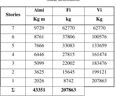
∑𝑛_𝑖=1(𝑚_𝑖𝛥_𝑖) Equation 24. (Other floors shear distribution) Table 6. Shear distribution. Stories Δimi Fi Vi Kg m kg Kg 7 9729 62770 62770 6 8761 37806 100576 5 7666 33083 133659 4 6446 27815 161474 3 5099 22002 183476 2 3625 15645 199121 1 2026 8742 207863 Σ 43351 207863

𝑂𝑇𝑀 = ∑ 𝐹𝑖 𝐻𝑖 Equation 25. (Base Overturning Moment) Table 7. Overturning moments Stories Hi Fi OTM (m) Kg Kg-m 7 21,5 62770 0 6 18,5 100576 188310 5 15,5 133659 490038 4 12,5 161474 891015 3 9,5 183476 1375437 2 6,5 199121 1925867 1 3,5 207863 2523230 Base 0 0 3250750

(37)

17

2.2.3.3. P-Δ Effect

In steel structures the P-Δ effect must be consider if the stability index is great than 0.05 for values less than 0.05 this effect can be ignoring.

Moreover, another aspect to consider is that 0.3 is the maximum value of the stability index; if the value is great than 0.3, the structure must be redesign to increase the stiffness of the structure.

Taking in count the P-Δ, the base shear and overturning moment must be increased depending of the structural material. A simple method to reflect the P-Δ effect in the base shear distribution and overturning moments is to multiply the values of this parameters by a coefficient. The coefficient is equal to the increased base shear by the P-Δ effect divided by the based shear without P-Δ effect

θΔ= PΔ_d

VHe or θΔ=

PΔ_d

𝑂𝑇𝑀 Equation 26. (Stability index) 𝜃Δ=0.1564 (first formula)

𝑉_𝑏(P−Δ)= 𝐹 = 𝐾_𝑒𝛥_𝑑+ 𝐶𝑃𝛥𝑑

𝐻_𝑒 Equation 27. (Based shear increased by P-Δ effect) Vb(P-Δ) = 435746 Kg

𝐴 =𝑉𝑏(P−Δ)

𝑉_𝑏 Equation 28. (Amplification factor)

A= 1.16

(38)

18 Table 8.

Increased lateral floor by P-Δ effect

Stories Fi(P-Δ) Vi(P-Δ) kg Kg 7 73017 73017 6 43978 116995 5 38484 155478 4 32356 187834 3 25594 213428 2 18199 231627 1 10169 241796 Σ 241796

𝑂𝑇𝑀𝑖(P−Δ) = 𝑂𝑇𝑀𝑖 𝐴 Equation 30. (Increased overturning by P-Δ effect) Table 9. Overturning by P-Δ effect Stories OTM(P-Δ) Kg-m 7 0 6 219051 5 570035 4 1036469 3 1599971 2 2240256 1 2935136 Base 3781420

Comparison of results obtained from DBDD

with FBD.

In order to compare de displacement method with the forced and displacement methods, the elements of the structure were design with the lateral force obtained by the direct based

(39)

19 design and the linear static seismic lateral force (forced method) according the AISC 360, 341, and 358.

The structure is classified as a special moment frame which was a reduction seismic response modification factor (R) equal to 8. Also in both cases, the maximum drift was 0.025; the two analysis included the P-delta effect.

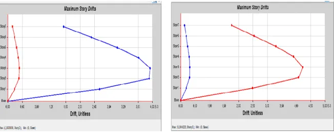
Figure 8. Maximum drift in force design a) Lateral force in X B) Lateral force in Y

𝛥𝑚𝑎𝑥 = 0.78 𝑅 𝛥 Equation 31. (Maximum inelastic interstory drift according NEC 15) Δ = 0.025

Figure 9. Maximum drift in displacement design a) Lateral force in X B) Lateral force in Y

(40)

20

2.3.1. Quantity of steel obtained.

All structural elements are classified as high ductility section, and the design satisfy limit state design (LRF) for ultimate and serviceability limit state. The final sections are present in table 10.

Table 10.

Final element sections.

DBDD BFD

Web Flange Web Flange Element h th b tb h th b tb cm cm cm cm cm cm cm Cm C1 60 2 35 2 65 2 35 2 VM1 50 1 20 1,2 45 0,8 18 1,5 VM2 35 0,8 12 1 40 0,8 12 1 VP1 50 1 20 1,5 45 0,8 24 1,5 VS 16 0,4 9 0,6 17 0,4 9 0,6 Table 11.

Total weight for force and displacement design

Total Weight Element Type DBDD DBF kgf kgf Column 90230,1 98112,84 Beam 121705,31 119116,71 Σ 211935,41 217299.55

Table number 12 shows that the structure design with the displacement method presents a 2.54% less material than the traditional force design.

(41)

21

2.3.2. Base shear and lateral forces.

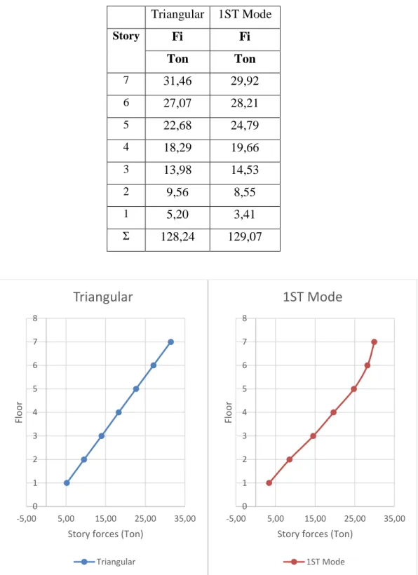
The base shear distribution in the lateral force has a triangular configuration due to the regularity of the building; in the case of the displacement method the story force was obtained by DBDD. The lateral forces are equal for the axes X and Y. The lateral forces were applied with a 5% of eccentric that stipule the Ecuadorian and international codes.

Table 12.

Comparison of lateral forces between displacement and force method.

DBDD BFD

Story Location Elevation Force Force Variation

m tonf tonf % Story7 Top 21,5 73,159 51,732 41,421 Story6 Top 18,5 44,063 44,983 -2,046 Story5 Top 15,5 38,558 36,962 4,317 Story4 Top 12,5 32,419 29,111 11,363 Story3 Top 9,5 25,644 21,528 19,121 Story2 Top 6,5 18,234 14,167 28,706 Story1 Top 3,5 10,189 7,161 42,281 Σ 242,266 205,644

The base shear in the displacement methods is 17.8% greater than the obtained with the force method; similarly, the story forces are greater in all stories except the story six where the force decrees two percent. The reduction in the story six is product of the consideration of the high mode.

(42)

22

3. Fluid viscous damper

Introduction

All the structures that are submitted to dynamic actions such as seismic events responses to them dissipating the seismic input energy; this balance of energy is expressed in equation 33.

𝐸𝑖 = 𝐸𝑘+ 𝐸𝑠+ 𝐸ℎ+ 𝐸𝜉Equation 32. (Balance energy equation)

The input energy from the seismic event (Ei) is equal to the kinetic energy (Ek), elastic deformation energy (Es), plastic deformation energy dissipated kwon as hysteretic (Eh), and the viscous damping dissipation (Eξ) proper of the structure and by the additional system (Colunga, 2003). The most common solution that the engineers select to balance the equation is to increase the elastic and inelastic response by incising the structural element cross sections and the quantity of steel. In the last decades, the used of dampers and isolation system increasing the viscous damping. The additional systems dampers and insulators can be classified in three classes:

 Passive Control Systems: These systems are mechanical devices which does not require a power source to active; on other hand, their functioning start with the deformation, or acceleration of the structure that produce a movement of the devices dissipating energy. Their functioning cannot be controlled, and it only depends of the response of the structure. The passive systems are the cheapest system of the three classes of system; in this group are the mechanisms that working with the yielding of mild steel, viscoelastic action in rubber-like materials, sloshing of fluid, shearing of viscous fluid, orificing of fluid, and sliding friction (Symans, Constantinou, Taylor, & Garnjost, 2012)

 Active Control Systems: Electro-hydraulic compose of movement sensors, process data system and hydraulic components. The devices started at the same moment in which the seismic event stars; the sensor sent a signal and the quantity of

displacement after the system of process data calculate the necessary for to be applied in the hydraulic system to counter the seismic effects, and the hydraulic

(43)

23 system applies the calculated force. These systems need a large external power sources, and their maintenance cost are high.

 Semi-Active Control Systems: These systems require small quantities of external power. The semi-active system acts as an active control system with small seismic vent or wind effect, and they act as a passive system with strong seismic events.

Fluid viscous dampers

The fluid viscous dampers (FVD) are a passive energy dissipation; also, the FVD are used in a complement in the isolation system too. These dampers are more common used in the rehabilitation to achieve a determine performance with a define demand; in the last two decades the system has been implemented in design of new building obtaining smaller transversal section in the structural element, better performance and less developing of plastic hinge during the seismic events, wind storms, or blasts (Teresa, 1999).

The fluid viscous dampers increase the critical damping ration of the structure that commonly is equal to five percent in structures without complement systems reducing the dynamic response of the system; theses system takes the majority of the input energy remaining the majority of the structure inside of the elastic limits, and only a few plastic hinges.

3.2.1. Fluid viscous dampers parts and working.

The FVDs is composed of a stainless-steel piston rod with a bronze orifice head and a self-contained piston displacement accumulator. The damper cylinder is filled with a compressible viscous fluid (silicone or oil) which is generally non-toxic, non-flammable, thermally stable and environmentally safe. (Narkhede & Sinha, 2012)

(44)

24

Figure 10. Longitudinal section of fluid viscous damper

During the seismic event, the fluid flow through orifices due to the difference of pressure between the two cavities inside the FVDs. The flow of the fluid produces friction between the fluid, the piston and the walls of the chamber, and the movement of the fluid produces an increasing of the temperature (Heat) inside of the damper. Also, the compressive behavior prudes a change of the volume simulating a spring with a restoring force. The energy dissipation in this system is in form of heat that is dissipates into the atmosphere, friction and the compression in the fluid.

The force in the viscous damper is given by, F = C.Vα where F is the output force, V the relative velocity across the damper, C is the damping coefficient and α is a velocity constant exponent which is usually a value between 0,3 and 1,0. Fluid viscous dampers can operate over temperature fluctuations ranging from –40°C to +70°C. (SaiChethan, Srinivas, & Ranjitha, 2017)

(45)

25 The response of the fluid viscous damper is out of phase with the structure movement and tension, so the devices do not add stress to the structure. The dampers are velocity dependent. The maximum tensions are developed at maximum lateral displacement, and the velocity is zero at that point. The maximum velocity is reached when the structure pass through rest position. (Brown, M. Uno, Thompson, & Stratford, 2015)

Figure 12. Force displacement relationship

(46)

26

3.2.2. Fluid viscous dampers configuration and

location.

The configuration of the FVDs has a great influence in the efficiency of the force develop by the device. The angle that form the braced with the horizon axis, vertical axis or with the other components of the brace that contain the damper. In the figure 12 are present the consideration to take in count in the configuration of the dampers.

Figure 14. FVDs efficiency by their configuration. Source: (Castro & Sánchez, 2016)

Analyzing table figure 12, the configuration chevron has one of the better efficiencies sending the total horizontal force developing in the system to the structure, but if it considers the vertical component of the seismic effect, the chevron configuration is not able to counter in any percentage the vertical component giving to the other configurations an advantage. Another aspect to consider, it is the quantity of steel used in which the better configuration is the simple brace. The code ASCE 7 in the chapter eighteen gives recommendation for the location of the dampers:

 It is recommendable that the structure does not present irregularities.

 In every level, it must be at least two dampers in the direction to reinforce.

(47)

27

 It is recommendable that the location of the dampers will be symmetrical in order to not generate torsion.

In order to obtain the optimal location of the dampers, the design and analysis procedure should be an iterative process considering the architecture and used of the building.

3.2.3. Procedures for the design of the FVDs

The American Society of Civil Engineers in the code ASCE 7 in the chapter eighteen recommends the use of four procedures two non-lineal and two lineal. The ASCE 7 and the NEC allow the use of artificial records or accelerogram compatibles in the case of lacking accelerograms recorded in area of the study case.

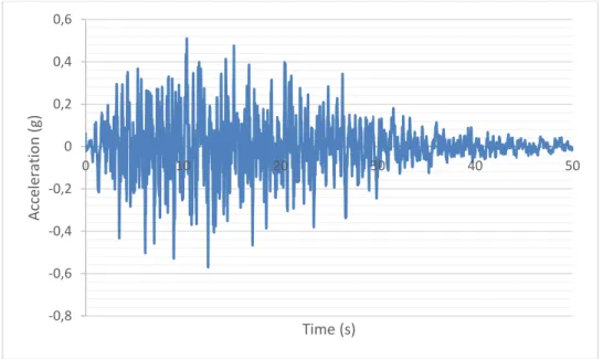
For these cases, the non-linear response time-history will be used, and it was generated synthetic based in the geology and soil conditions of Quito and the area where was determine to implement the structure. Similarly, three synthetic accelerograms were generated for the non-lineal dynamic analysis that is the minimum establish in ASCE, NEC, and Eurocode.

3.2.4. Fast Nonlinear Analysis (FNA)

The Fast-Nonlinear Analysis (FNA) is a modal time history analysis that can be lineal or non-lineal. The modal analysis is done by modal superposition, and the obtaining of the N number of modal modes is with Ritz-vectors. The analysis only takes in count the nonlineal behavior in limited elements selected, and elements with concentrated damping, base isolation or energy dissipation.

Mü(t) + C𝑢̇(𝑡) + 𝐾𝑢(𝑡) + 𝑅(𝑡)𝑁𝐿= 𝑅(𝑡) Equation 33. FNA general equation

In the equation 34, M, C and K are the mass, proportional damping and stiffness matrices, respectively. The elastic stiffness matrix K omit the stiffness of nonlinear elements. The R(t)NL is the global node force vector from the sum of the forces in the nonlinear elements and is computed by iteration at each point in time.

It can be added to equation 34 a matrix of arbitrary stiffness Keu(t) of random value in the both size of the equation if the structure is unstable without the nonlinear element.

(48)

28 The introduction of the effective stiffness elements will eliminate the introduction of long periods into the basic model and improve accuracy and rate of convergence for many nonlinear structures. (Wilson, 1995)

Mü(t) + Cu̇(t) + (K + Ke)u(t) = R(t) − R(t)NL+ Ke u(t) Equation 34. (FNA general equation 2)

Using the Ritz-vector, the modal analysis and the transformation to modal coordinates can be done obtaining equation 36.

IŸ(t) + ΛẎ(t) + ΩY(t) = F(t) Equation 35. (Ritz-vector equation)

The term F(t) is the lineal and nonlinear forces acting in the system.

F(t) = Ф𝑇_{𝑅(𝑡) − Ф}𝑇_𝑅(𝑡)

𝑁𝐿+ Ф𝑇𝐾𝑒𝑢(𝑡) Equation 36. (Total forces in the sys FNA)

The FNA reduces the computational time required for a nonlinear dynamic analysis of a large structure, with a small number of nonlinear elements, can be only a small percentage more than the computational time required for a linear dynamic analysis of the same structure. This allows large nonlinear problems to be solved quickly (Wilson, 1995)

3.2.5. Constants and coefficients determination of

FVDs

In order to determine the dampers and their producing force, it is required to define the velocity coefficient, damping constants and necessary damping of the structure to reach the displacement target.

𝐹 = 𝐶𝑉 Equation 37. (FVD force.)

The viscous damping of the structure depends of the damping constants of the dampers, configuration of the FVD, and structure mass, relative displacement of the damper’s extremes, angular frequency and the last story displacement in the fundamental mode. The equation 39 is taken from the FEMA 274, and solving the equation can define the damping coefficient.

(49)

29 _H = ∑CjФrj 1+_cos1+_θ j j 2πA1−ω2−∑imiΦ𝑖2

Equation 38. (Structure viscous damping)

∑Cj =

_H2πA1−ω2−∑imiΦ𝑖2

∑jФ_rj1+cos1+θj

Equation 39. (Damping coefficient)

The maximum displacement is obtaining from the time history analysis, and the target displacement is taken from the local code. Determining the target and the maximum displacement, the target damping can be computed, and this damping will be the approached in the interactive process.

𝐵 = 𝐷𝑚𝑎𝑥

𝐷𝑡𝑎𝑟𝑔𝑒𝑡 Equation 40. (Reduction factor B function of drift)

𝐵 = 2.31−0.41ln (𝛽0)

2.31−0.41ln (𝛽𝑒𝑓𝑓) Equation 41. (Reduction factor B function of damping)

𝛽_{𝑑𝑎𝑚𝑝𝑒𝑟} = 𝛽_𝑒𝑓𝑓− 5% Equation 42. (Viscous damping of the dampers.)

The parameter  is function of the modal participation factor ( Γ ), and the velocity constant exponent (  ). The parameter  can be computed from a formula or a table in the FAME 274. = 22+ Γ2(1+  2 ) Γ(2+) Equation 43.  (Formula.) Table 13 Values of parameter. Exponent  Parameter  0,25 3,7 0,5 3,5 0,75 3,3 1 3,1 1,25 3 𝐴 =𝑔𝑥Г𝑖𝑥𝑆𝑎𝑥𝑇

(50)

30 Finally, it is necessary to determine an adequate steel profile annex to the damper that does not bend of produce flexure reducing the efficiency of the FVD. The steel profiles HSS and pipes are the most common for this propose.

Fluid viscous dampers application.

The structures designed with the force and this placement method were design with a superior story drift that is defined in the code. The exceeded quantity will be reduced with damper. The force and displacement model are similar the analysis and design of the damper will be performed in one.

3.3.1. Non-lineal time history analysis without

dampers.

According with the geological, geotechnical, and the soil type were generating three synthetic accelerogram. Three accelerogram is the minimum of the registers establish in the North American and Ecuadorian code.

Figure 15. Artificial accelerogram 1. -0,8 -0,6 -0,4 -0,2 0 0,2 0,4 0,6 0 10 20 30 40 50 Acc ele ra tio n (g) Time (s)

(51)

31

Figure 16. Artificial accelerogram 2.

Figure 17. Artificial accelerogram 3.

Figure 18. Matching accelerogram 1 with response spectra -0,6 -0,4 -0,2 0 0,2 0,4 0,6 0,8 0 10 20 30 40 50 Acc ele ra tio n (g) Time (s)

Accelerogram 2

-0,6 -0,4 -0,2 0 0,2 0,4 0,6 0 10 20 30 40 50 Acc ele ra tio n (g) Time (s)

Accelerogram 3

(52)

32

Figure 19. Matching accelerogram 2 with response spectra

Figure 20. Matching accelerogram 3 with response spectra

Obtaining the artificial accelegrams, they were matching with the elastic spectra. In order to load case for the time history analysis with components X and Y, the accelerograms were combining taking the hundred percent for one direction and thirty percent in the perpendicular direction.

Table 14.

Maximum and minimum drifts X direction.

Story TH1,1 TH1,2 TH1,3 TH1,4 TH1,5 TH1,6

Max Min Max Min Max Min Max Min Max Min Max Min

Story7 0,0121 0,0111 0,0115 0,0138 0,0119 0,0117 0,0016 0,0019 0,0036 0,0035 0,0036 0,0033 Story6 0,0173 0,0171 0,0165 0,0190 0,0166 0,0166 0,0022 0,0026 0,0050 0,0050 0,0052 0,0051 Story5 0,0210 0,0217 0,0213 0,0226 0,0200 0,0209 0,0029 0,0031 0,0060 0,0063 0,0063 0,0065 Story4 0,0238 0,0239 0,0244 0,0252 0,0241 0,0245 0,0033 0,0034 0,0072 0,0074 0,0071 0,0072 Story3 0,0268 0,0256 0,0250 0,0260 0,0256 0,0278 0,0034 0,0035 0,0077 0,0083 0,0080 0,0077 Story2 0,0264 0,0255 0,0242 0,0241 0,0251 0,0268 0,0033 0,0033 0,0075 0,0080 0,0079 0,0076 Story1 0,0160 0,0154 0,0143 0,0147 0,0163 0,0157 0,0019 0,0020 0,0049 0,0047 0,0048 0,0046

(53)

33 Table 15.

Absolute maximum drifts X direction.

Story Elevation TH1,1 TH1,2 TH1,3 TH1,4 TH1,5 TH1,6 Max m Story7 21,5 0,0121 0,0138 0,0119 0,0019 0,0036 0,0036 0,0138 Story6 18,5 0,0173 0,0190 0,0166 0,0026 0,0050 0,0052 0,0190 Story5 15,5 0,0217 0,0226 0,0209 0,0031 0,0063 0,0065 0,0226 Story4 12,5 0,0239 0,0252 0,0245 0,0034 0,0074 0,0072 0,0252 Story3 9,5 0,0268 0,0260 0,0278 0,0035 0,0083 0,0080 0,0278 Story2 6,5 0,0264 0,0242 0,0268 0,0033 0,0080 0,0079 0,0268 Story1 3,5 0,0160 0,0147 0,0163 0,0020 0,0049 0,0048 0,0163 Table 16.

Maximum and minimum drifts Y direction.

Story TH1,1 TH1,2 TH1,3 TH1,4 TH1,5 TH1,6

Max Min Max Min Max Min Max Min Max Min Max Min

Story7 0,002 0,0021 0,0043 0,0037 0,0041 0,0047 0,0136 0,0156 0,0147 0,0155 0,0142 0,0125 Story6 0,0027 0,0028 0,0056 0,0051 0,0056 0,0063 0,0188 0,0209 0,0201 0,0206 0,0186 0,0171 Story5 0,0033 0,0033 0,0068 0,0067 0,0073 0,0073 0,0242 0,0243 0,0247 0,0248 0,0228 0,0223 Story4 0,0037 0,0036 0,008 0,008 0,0083 0,0083 0,0276 0,0276 0,0272 0,0269 0,0267 0,0265 Story3 0,0037 0,0038 0,0086 0,0085 0,0082 0,0086 0,0274 0,0285 0,0273 0,0284 0,0286 0,0283 Story2 0,0032 0,0036 0,0084 0,008 0,0076 0,0076 0,0252 0,0254 0,024 0,0267 0,0279 0,0265 Story1 0,0019 0,0021 0,0047 0,0046 0,0043 0,0042 0,0143 0,0141 0,014 0,0154 0,0158 0,0152 Table 17.

Absolute maximum drifts Y direction.

Story Elevation TH1,1 TH1,2 TH1,3 TH1,4 TH1,5 TH1,6 Max m Story7 21,5 0,0021 0,0043 0,0047 0,0156 0,0155 0,0142 0,0156 Story6 18,5 0,0028 0,0056 0,0063 0,0209 0,0206 0,0186 0,0209 Story5 15,5 0,0033 0,0068 0,0073 0,0243 0,0248 0,0228 0,0248 Story4 12,5 0,0037 0,0080 0,0083 0,0276 0,0272 0,0267 0,0276 Story3 9,5 0,0038 0,0086 0,0086 0,0285 0,0284 0,0286 0,0286 Story2 6,5 0,0036 0,0084 0,0076 0,0254 0,0267 0,0279 0,0279 Story1 3,5 0,0021 0,0047 0,0043 0,0143 0,0154 0,0158 0,0158

After performing the Time History Fast Non-Lineal Analysis in the structure, the maximum drifts were obtaining. In the X and Y axes, the absolute maximum drifts are equal to 0.278 and 0.286 respectively. In both cases, the maximum drift of the time history analysis

(54)

34 is greater than the maximum drift establishes in the Ecuadorian code and the obtaining of the static force analysis. The viscous damper will be used to get the target drift without changing the structural configuration of the building.

3.3.2. Determination of FVDs parameters.

The first pass is to calculate the reduction factor with the obtained maximum and with the target displacement. The reduction factor allows to get a first quantity of damping in the iterative that the devices will have to add to the system. It is necessary to reduce the self-damping of the structure that is taken five percent commonly.

𝐵 = 𝐷𝑚𝑎𝑥 𝐷_{𝑡𝑎𝑟𝑔𝑒𝑡} 𝐵 =0.278

0.20 = 1.39 Reduction factor X axes 𝐵 =0.286

0.20 = 1.43 Reduction factor Y axes

𝛽_𝑒𝑓𝑓 = 𝑒 (0.41 ln(𝛽0)−2.31_𝐵 )+2.31 0.41 𝛽_𝑒𝑓𝑓 = 15.47% Factor X axis 𝛽_{𝑑𝑎𝑚𝑝𝑒𝑟} = 15.47 − 5 = 10.47% Factor X axis 𝛽_𝑒𝑓𝑓 = 16.77% Factor Y axis 𝛽_{𝑑𝑎𝑚𝑝𝑒𝑟} = 16.77 − 5 = 11.77% Factor Y axis

Two models are going to be design with two different dampers. The first one is with a velocity constant equal to 0.5, and the second one with a constant equal to one known as lineal damper. In the two cases, the number of dampers placed are two for each direction accomplish with the requirements of the ASCE 7.