Backtesting Value-at-Risk Models

(1)

i

School of Economics and Management

University of Minho

Backtesting Value-at-Risk Models

Dissertation Master in Finance

2016/2017

Supervisor: Professor Nelson Areal

By:

(2)

iii Acknowledges

I would like to thank Mr. Nelson Areal for his guidance, helpful comments, suggestions and patience through all the process, his help was fundamental. Also I would like to thank to my friends, girlfriend and family for their constant support and motivation.

(3)

(4)

v Abstract

In the last decades, Value-at-Risk has become one of the most popular risk measurements techniques in the financial world. However, VaR models are only useful if they predict risk accurately. In order to evaluate the quality of the VaR estimates, it is necessary to perform appropriate and diverse backtesting methodologies.

In this study I test VaR estimates obtained from an unconditional parametric models (student-t generalized error, skewed student-t, pareto, and Weibull distributions) for four stock market indexes (DJIA, SP-500, Nikkei 225 and Dax 30) considering several different confidence levels. A rolling function procedure is applied to estimate the models parameters through maximum likelihood.

The performance of the VaR models is measured by applying several different tests of Unconditional Coverage, Independence and Conditional Coverage.

The results of the backtests provide some indication of the possible problems of the models, being the main one the independence property, leading us to conclude that they do not react well under high turbulent times, and consequently exceptions are auto correlated and come in clusters.

Title: Backtesting Value-at-Risk models Author: Pedro Rodrigues

Department: Management Major subject: Financial Risk

(5)

(6)

vii Resumo

Durante as ultimas décadas, Value-at-Risk tornou-se uma das medidas de risco mais populares na industria financeira. Todavia, os modelos VaR só são úteis se conseguirem fazer uma previsão acertada do risco. De forma a avaliar a qualidade e precisão das estimativas de um modelo VaR, é necessário utilizar uma metodologia apropriada de avaliação.

A principal contribuição desta dissertação consiste em estudos empíricos, onde diversos modelos VaR paramétricos não condicionais são estimados para os quarto índices selecionados assumindo, para cada um, utilizando um leque de cinco distribuições: Student t, Generalized Error, Skewed Student t, Pareto e Weibull. Os parâmetros dos modelos são estimados por máxima verosimilhança através de uma janela rolante.

A performance das estimativas VaR é medida aplicando testes de cobertura incondicional, independência e cobertura condicional.

Os resultados da avaliação aos modelos mostrou alguns problemas, sendo o mais grave a falta de independência entre as excepções, levando-nos a concluir que os modelos não reagem bem durante períodos turbulentos, e consequentemente as excepções surge em grupos e estão bastante correlacionadas.

(7)

(8)

ix Index Acknowledges……….. iii Abstract ……….………..………….. v Resumo ……….………... vii Index ……… ix List of Figures ……….……… xi 1. Introduction …………..……….. 1 1.1 Background ..………1 1.2 Objective ……….……2 1.3 Structure ………..………...….3

2. Value-at-Risk Literature Review ……….4

2.1 History of VaR ………..4

2.2 Defining VaR ……….4

2.3 Different Approaches to VaR ………..7

2.4. Backtesting Procedures ……….………..11

2.4.1 Unconditional Coverage ….………11

2.4.2 Independence Test …….………..……….12

2.4.3 Conditional Coverage ……….13

2.4.4 Multiple VaR levels ………..13

2.4.5 Loss Function ………14

3. Methodology………15

3.1 Daily returns ………..15

3.2 VaR – Unconditional Parametric Estimation ……….15

3.3 Returns Distributions ………..16 3.3.1 Student t ……….16 3.3.2 Generalized Error ………16 3.3.3 Skewed Student t ………17 3.3.4 Pareto ………..18 3.3.5 Weibull ……….18

(9)

x 3.4 Backtests ……….18 3.4.1 Unconditional Coverage ………19 3.4.2 Independence ………..20 3.4.3 Conditional Coverage ……….22 4. Data ………..24 5. Results ……….28 5.1 VaR Calculation ……….28

5.1.1 Unconditional Parametric Estimation ...………..28

5.2 Backtests ……….39 5.2.1 Unconditional Coverage ………39 5.2.2 Independence ………..43 5.2.3 Conditional Coverage ……….46 6. Conclusions ………50 Bibliography ………52

(10)

xi List of Figures

Figure 1: VaR for Normal distribution ……….6

Table 1: Basic stats of the four indexes ….………24

Figure 2: Dow Jones Industrial index returns ………25

Figure 3: S&P 500 index returns ………26

Figure 4: Nikkei 225 index returns …….………..26

Figure 5: Dax 30 index returns ………27

Figure 6: Dow Jones Industrials VaR Unconditional Parametric approach under Student t…...29

Figure 7: S&P 500 VaR Unconditional Parametric approach under Student t………..…...29

Figure 8: Nikkei 225 VaR Unconditional Parametric approach under Student t………..…...30

Figure 9: Dax 30 VaR Unconditional Parametric approach under Student t………..…...30

Figure 10: Dow Jones Industrials VaR Unconditional Parametric approach under GED…….…....31

Figure 11: S&P 500 VaR Unconditional Parametric approach under GED………...31

Figure 12: Nikkei 225 VaR Unconditional Parametric approach under GED…..………..…...32

Figure 13: Dax 30 VaR Unconditional Parametric approach under GED…..………..…...32

Figure 14: Dow Jones Industrials VaR Unconditional Parametric approach under SST…….…...33

Figure 15: S&P 500 VaR Unconditional Parametric approach under SST………...33

Figure 16: Nikkei 225 VaR Unconditional Parametric approach under SST…..…….………..…...34

Figure 17: Dax 30 VaR Unconditional Parametric approach under SST…..………..…...34

Figure 18: Dow Jones Industrials VaR Unconditional Parametric approach under Pareto……...35

Figure 19: S&P 500 VaR Unconditional Parametric approach under Pareto ………...35

Figure 20: Nikkei 225 VaR Unconditional Parametric approach under Pareto …….………..…...36

Figure 21: Dax 30 VaR Unconditional Parametric approach under Pareto ………..…...36

Figure 22: Dow Jones Industrials VaR Unconditional Parametric approach under Weibull..…...37

Figure 23: S&P 500 VaR Unconditional Parametric approach under Weibull………...37

Figure 24: Nikkei 225 VaR Unconditional Parametric approach under Weibull…….………..…...38

Figure 25: Dax 30 VaR Unconditional Parametric approach under Weibull………..…...38

(11)

xii

Table 3: S&P 500 Unconditional Coverage Test ………..40

Table 4: Nikkei 225 Unconditional Coverage Test ………..41

Table 5: Dax 30 Unconditional Coverage Test ……….….41

Table 6: Dow Jones Independence Test ……….44

Table 7: S&P 500 Independence Test ……….44

Table 8: Nikkei 225 Independence Test ……….45

Table 9: Dax 30 Independence Test ……….45

Table 10: Dow Jones Conditional Coverage Test ………..……..47

Table 11: S&P 500 Conditional Coverage Test ……….……..47

Table 12: Nikkei 225 Conditional Coverage Test ………..……..48

(12)

1 1. Introduction

1.1 Background

During the last two decades, Value-at-Risk (also known as VaR) became one of the most popular risk measurement techniques in finance. VaR is a method that aims to capture the downside risk of a single asset or a portfolio of assets. By definition, VaR measures the maximum loss in value of an asset/portfolio over a predetermined time for a given confidence interval.

Despite the common acceptance and use of VaR as a risk management tool, it has frequently been criticized for being incapable to produce reliable risk estimates. When implementing VaR systems, there will always be numerous simplifications and assumptions involved. Moreover, every VaR model, attempts to forecast future asset prices using historical market data, which won’t necessarily reflect the future market environment.

Thus VaR models are useful only if they accurately predict future risk. In order to verify that the results acquired from VaR calculations are a consistent and reliable forecast, the models should always be submitted to backtest procedures with appropriate statistical methods. Backtesting is a procedure where actual profits and losses are compared to projected VaR estimates. Jorion (2005) refers to these tests as “reality checks”. If the estimates of the VaR model are not accurate, the model should be re-examined for incorrect assumptions, inaccurate modelling or wrong parameters.

A series of different testing methods have been proposed for backtesting purposes. The first, and most basic test, such as Kupiec’s (1995) point-of-proof (POF-test), focuses in examining the frequency of losses in excess of VaR. This called failure rate should be in line with the selected confidence level. For instance, if daily VaR estimates are computed at 95% confidence level for one year (with generally has 250 trading days), we would expect, on average, 12.5 VaR violations, or exceptions, to occur during this period, not more, not less. In the POF-test we would then examine whether the actual failure rate is reasonable when compared to the predicted amount.

In addition to the acceptable proportion of exceptions, another equally important aspect is to make sure that the observations exceeding VaR levels are independent and evenly spread over time. A good VaR model is one that is capable of avoiding exceptions clustering by reacting quickly to changes in financial assets volatilities and correlations. These types of tests, that take into account

(13)

2 the independence of exceptions were first suggested by Christoffersen (1998) and later by Hass (2001). These tests come as a complementary measure to the regulatory backtesting framework proposed by the Basel Committee (1996).

Backtesting is, or at least should be an integral part of VaR reporting in current risk management practices. Without a proper model validation process, one can never be sure that the VaR system yields accurate risk estimates. This subject is especially important in the current market environment where volatile market prices tend to make investors more interested in portfolio risk figures as losses accumulate. Although the common widespread and acceptance of VaR, it is known to have severe problems in estimating losses at times of turbulent markets. As a matter of fact, by definition, VaR measures the expected loss only under normal market conditions as said by Jorion (2005). This limitation is one of the major disadvantages of VaR and it makes model forecast and backtesting procedures very challenging and interesting as will be shown latter in this dissertation.

1.2 Objective

The main objective of this dissertation consists in performing an empirical study. However, in order to provide an exhaustive description about the modelling and the backtesting processes in the empirical part, I will first discuss VaR in general and the theory of the main models and backtesting methods currently available. In the literature review we aim to provide the reader with some of the most common procedures used to calculate VaR and to backtest it.

The objective of the empirical study here performed, is to uncurtain which of the tested distributions yield the best VaR estimates under an unconditional parametric approach, for each of the indexes here considered.

Methodological issues will not be covered in great detail, meaning that the reader is assumed to be familiar with statistical decision theory and related mathematics to some extent.

1.3 Structure

The thesis consists of seven chapters, of which the first one is the introduction. The second chapter starts with describing the basic idea behind VaR and gives some background and history on the

(14)

3 subject, also including some of the general advantages and shortcomings reported in the literature. The second chapter, also presents the forecasting procedures. Several methods are presented, and the advantages and disadvantages throughout the literature are shown. The aim of the discussion is to focus on the most common VaR estimation methods, and especially on those that will be applied latter on. The last subsection of the second chapter focus on the backtesting methods. Some of the backtests available are presented in detail, but the discussion is by no means exhaustive, since it is impossible in this context to go through the panoply of different methods and their applications. I will discuss more in concert the methods applied later on, which are the ones mostly used in the literature.

The fourth chapter presents the detailed methodology behind the methods used in this dissertation, providing the formulas and procedures in detail. In fifth chapter data is presented, along with some descriptive statistics.

The sixth chapter forms the empirical part of the dissertation, and as such, can be considered the core of the study. Some of the methods presented in the preceding chapters, are applied to actual VaR calculations, and thereafter to their backtesting. The results are discussed in detail and the factors affecting the outcome are analysed thoroughly.

The seventh and last chapter is the conclusion. The most significant results are explained, discussed and compared to the existing literature.

(15)

4 2. Literature Review

2.1 History of VaR

In the past decades, risk management has evolved to a point where it is considered to be a distinct sub-field in the theory of finance. The growth of the risk management industry traces its roots back to the increased volatility of financial markets in 1970’s. The breakdown of Bretton Woods system of fixed exchange rates and the fast pace on the development of new theories, such as adoption of Black-Scholes model, were among the important events that contributed to the revolution in risk management as stated by Dowd (1998). Another factor that is pointed by Dowd (1998) is simply the increase of the trading activity. For example, the average number of shares traded per day grew from 3.5 million in 1970 to 40 million in 1990. Equally impressive is the growth of the dollar value of outstanding derivatives positions, that went from $1.1 trillion in 1986 to $72 trillion in 1999 as presented by Jorion (2005). These factors combined with the unpredictable events of the 1990s, such as the financial disasters in Metallgesellschaft, Barings Bank, Orange County, Daiwa, “dot com bubble” and the “currency crisis” highlighted the danger allocated to financial positions and stimulated the need of improved internal risk management tools (Jorion 2005).

The mathematical roots of VaR calculation were developed already in the context of portfolio theory by Harry Markowitz and others in the 1950s. Financial institutions began to construct their own risk management models in the 1970s and 1980s, but it was not until the ground-breaking work from J. P. Morgan through the RiskMetrics model in 1994 that made VaR the industry-wide standard. (Dowd 1998). During this process, also regulators became interested in VaR. The Basel Accord of 1996 came as an important mark as it allowed banks to use their own internal VaR models to compute their regulatory capital requirement (Linsmeier & Pearson, 1996). Since then, VaR has grown to become the dominant measure of market risk and it is likely to gain even more acceptance in the near future as the methods are improved further, with new approaches being able to better estimate VaR.

2.2 Defining VaR

Companies face many different kinds of risks, such as market risk, liquidity risk, credit risk, counterparty risk, model risk, and estimation risk. VaR was original developed to measure market risk, which is caused by movements in the level or volatility of asset prices, but it was soon realized

(16)

5 that VaR methodology could also be applied to measure other types of risks, like liquidity risk and credit risk as stated by Jorion (2005). According to Dowd (1998) the market risk can be subdivided into four classes: interest rate risk, equity price risk, exchange risk and commodity price risk. Philippe Jorion (2005) states that “VaR measures the worst expected loss over a given horizon under normal market conditions at a given level of confidence. For example, a bank might say that the daily VaR of its trading conditions, only one percent of the time, the daily loss will exceed $1 million.”

The basic idea behind VaR is very straightforward since it gives a simple quantitative measure of portfolio’s downside risk. VaR has two important and appealing characteristics. The first one is that it provides a common consistent measure of risk for different positions and instrument types. Second, it takes into account the correlation between different risk factors. This property is absolutely essential whenever computing risk figures for a portfolio of more than one instrument Dowd (1998).

Assuming that asset returns are normally distributed, VaR may be illustrated graphically as in Figure 1. In mathematical terms, VaR is calculated as follows:

𝑉𝑎𝑅_𝛼 = 𝛼 ∗ 𝜎 ∗ 𝑊 (1)

The α indicates the selected confidence level, σ the standard deviation of the portfolio returns and W the initial portfolio value. An example seen in Jorion (2005), considers the situation where initial portfolio value is €100 million and the portfolio returns have an annual volatility of 20%. Calculating the 10 day VaR at a confidence level of 99% gives us the following result:

𝑉𝑎𝑅_99% = −2.33 ∗ √(10

250) ∗ €100𝑀 ≈ −€9.3𝑀

(2)

Where the square root in this function represents the 10-day time horizon assuming there are 250 trading days. As can be seen above, VaR computation can be very straightforward if normality is assumed to prevail. The simplicity of this assumption comes with some severe drawbacks which will be discussed shortly.

(17)

6

Figure 1: VaR for Normal distribution. The graph illustrates the VaR for two confidence levels when portfolio returns are normally distributed. The values of μ can be read from the standard normal distribution tables.

When interpreting VaR figures, it is essential to keep in mind the time horizon and the confidence level, since without them, it is not possible to interpret VaR numbers. The investors that have actively traded portfolios such as financial firms, typically use 1-day time horizon, whereas institutional investors and non-financial firms, typically use longer horizons. Linsmeier & Pearson (1996) suggest that firms should select the holding period according to the length of time it takes to liquidate the portfolio. On the other hand, they must also take into account the properties of the calculation method. If methods based on the approximations are used, then a relatively short time horizon should be applied.

As for the choice of confidence level depends on the purpose of the model. If the objective is as in this case, a dissertation, to test different approaches to VaR, one should choose a high confidence level, but not a very high one, in order to be able to capture enough VaR violations. When assessing capital requirements, the confidence level depends on the risk aversion of senior management, were risk averse managers usually choose higher confidence levels. One additional aspect is to consider the possibility of comparing different VaR confidence levels with estimates from other sources, as Dowd (1998) suggests.

(18)

7 2.3 Different Approaches to estimate VaR

VaR calculation methods are usually divided into parametric and non-parametric models. Parametric models assume that returns follow a known probability distribution, whereas non-parametric models do not (Ammann & Reich 2001).

In this section I briefly present the basics of the most common VaR calculation methods. The following discussion is meant to be mainly descriptive as the focus is on the strengths and weaknesses of each method. Thorough mathematical presentations are beyond the scope of this short review and will only be presented for the methods that I will use.

One of the simplest forms of VaR is the Unconditional Parametric estimation. It specifies a parametric model for the unconditional distribution of returns and derives VaR from the quantile of this distribution. Its parameters can be estimated using Maximum likelihood and different parametric distributions can be used.

Initially most of the classical financial models, namely the Markowitz’s Portefolio Therory, the Capital Asset Pricing Model (CAPM) of Sharpe, Lintner and Mossin and the Black-Scholes’ formula required the assumption of normality and finite variance of financial asset returns. The Gaussinan hypothesis was not seriously questioned until the seminal papers of Mandelbrot (1963) and Fama (1965) which ignited numerous studies that latter found the empirical unconditional distribution of returns on financial data assets exhibit fatter tails and are more peaked around the center than would be predicted by a Gaussian distribution, i.e., the presence of leptokurtosis in the empirical distributions seems indisputable (Fama, 1965), and the variability of returns seems to be nonstationary. As a result, alternative distributions having such characteristics have been proposed as models for asset returns. Blattberg and Gonedes (1974) proposed Student t distribution, Box and Tiao (1962) and latter Nelson (1991) found evidence supporting the Generalized Error distribution, Wand et al. (2001) the exponential generalized beta distribution, Mittnik and Rachev (1993) the Weibull and double Weibull distribution, Fama (1965) Fama and Roll (1968) and So (1987) the Paretian distribution, Venkataraman (1997) the mixture of normal distributions as well as others.

Unconditional parametric is the natural analogue to historical simulation, which is using an empirical CDF to compute VaR instead of a model-estimated one. In particular, if the parametric model was unconditionally true, then it would be a better estimator than HS since it would have less uncertainty about the quantile than the non-parametric HS estimator.

(19)

8 The advantages and criticisms are identical to the parametric conditional VaR. The models are parsimonious and the parameters estimates are precise, yet finding a specification which necessarily includes the true distribution is a hard job as mentioned by Sheppard (2013) advises. Also, a distribution that may fit returns in one period, may be unfit in a different period. Finally returns may not even follow any known distribution as Bao et al. (2006) indicates.

J. P. Morgan back in 1992 released one of the VaR models that was most important to the spread of VaR usage. Its Riskmetrics realeased in 1992 became the most common and less restrictive conditional VaR, relying in a restricted generalized autoregressive conditional heteroscedasticity (GARCH) (1,1). This model includes no explicit mean model for returns and is only applicable to assets with returns that are close to zero or when the time horizon is short. This group has produced a surprisingly simple yet robust method for producing conditional VaR measure, but with some disadvantages being that, as Pafka & Kondor (2001) refer, it is based on the unrealistic assumption of normally distributed returns and completely ignores the presence of fat tails in the probability distribution, a most important feature of financial data. Also, several studies such as Danielsson & Vries (1997), Christoffersen (1998), and Engle & Manganelli (2004) have discovered relevant possible improvements when deviations from the relatively rigid RiskMetrics frameworks are explored, such as other models of the GARCH family.

Different types of autoregressive conditional heteroscedasticity models (ARCH), first introduced by Engle (1982), are commonly used to estimate risk. The ARCH model expanded into the GARCH model by Bollerslev (1986). These models capture the fluctuations in variance over time, which are present in most financial instruments. Another empirical observation is that the variance is usually higher during times of turmoil. Nelson (1991) created the exponential GARCH (EGARCH) model to capture this tendency. Nelson (1991) explains that an EGARCH model allows positive and negative shocks to have different effects on the estimated variance, he concludes, from empirical data, that the market volatility seem to react differently depending on the sign of the shocks, negative shocks usually result in periods of higher volatility compared to positive ones, and by his introduction of a third parameter the EGARCH allows the model to react differently depending on the different type of news.

The research in this area has been extensive. There is no definitive conclusion on which model in the GARCH family is best suited to forecast the volatility for specific types of securities. Most research has shown that a leptokurtic conditional distribution is better at describing the VaR

(20)

9 (Angelidis et al., 2004; Orchan and Köksal, 2011; Kösal, 2009; Aloui and Mabrouk, 2010). Usulally the normal distribution is compared against Student t or the generalized error distribution. A majority of research have concluded that models, that take into account information asymmetry, outperform symmetric models (Hansen and Lunde, 2005; Aloui and Mabrouk, 2010). When compared to other families of volatility models, the GARCH models outperforms others such as Black and Sholes models, stochastic volatility models, regime switching models and grey theorem (Lehar et al., 2002; Kung and Yu, 2008; Lou et al., 2010; Pederzoli, 2006).

The limitations that comes with this procedure are that implementations require knowledge of a density family, and that all the dynamics of returns can be summarized by a time-varying mean and variance, and so higher order moments must be time invariant as referred by Bekiros & Georgoutsos (2005) and Sheppard (2013).

Back in 1937, Cornish and Sir Ronald Fisher introduced the Edgeworth expansion, that in its most-used inverse form, relates the cumulative distribution function of a normal distribution to some distribution of interest. It later served as support to the Cornish-Fisher Approximation, that splits the difference between a fully parametric model and a semi-parametric model. It shares the strengths of the semi-parametric distribution in that it can be accurate without a parametric assumption. Unlike the semi-parametric estimator, the Cornish-Fisher estimators are not necessarily consistent which may be a drawback, and also that estimates of higher order moments of standardized residuals may be problematic or, in extreme cases the moments may not even exist as suggested by Christoffersen (1998).

As the purest form of a nonparametric estimate of the unconditional VaR comes Historical Simulation also known as HS, it is widely used in practice because of its very easy to implement. No numerical optimization must be performed because parameters don’t have to be estimated by maximum likelihood or any other method. Another advantage is its model free nature, because it does not rely on any particular parametric model such as the RiskMetrics model for variance and a normal distribution for the standardized returns. Historical Simulation lets the past data points speak fully about the distribution of next day’s return without imposing any further assumptions. It’s model free approach has the obvious advantage compared with model-based approaches that relying on a model can be misleading if the model is poor. Model-free nature also has several drawbacks of the method. Christoffersen (2012) describes mainly the that the choice of the data sample length is very ad hoc, and this influences the magnitude and dynamics of VaR. Another

(21)

10 drawback that comes from its modelfree nature is that as this method does not rely on well -specified dynamic model, there is no theoretical correct way of extrapolation from the 1-day distribution to get the 10-day distribution other than finding more past data as Christoffersen (2012) points out. Sheppard (2013) and Wiener (1999) consider Historical Simulation of being an unreliable method for the same reasons. More recently other variants of the HS have been preferred as the Weighted Historical Simulation and the Filtered Historical Simulation.

In order to overcome some of the disadvantages associated with the Historical Simulation, Barone-Adesi, F, & Giannopoulos (1998) and Barone-Adesi Giannopoulos, & Vosper (1999) introduce Filtered Historical Simulation. The procedure is considered non-parametric apart from assumptions used in the estimation of residuals in the GARCH process. It is one of the most highly reputed methods nowadays and one of the most used ones that suffered different innovations by several authors like Christoffersen, Barone-Adesi and Giannopoulos that with their approaches were able to correct several bias and often outperform the first generation VaR models. The clear advantage over their fully parametric ARCH cousins, is that the quantile, and hence the VaR, will be consistent under weaker conditions since the density of the standardized residuals does not have to be assumed. According to Hartz, Mittnik, & Paolella (2006) this method is also numerically extremely reliable. Pritsker (2001) and Kuester, Mittinik, & Paolella (2005) demonstrate de superiority of the FHS method in VaR estimation. Also Adcock, Areal, & Oliveira, (2011) concluded that the FHS is an accurate method to in order to forecast VaR in the presence of non-normal returns. However, the handicap is that the quantiles may be poorly estimated especially if the confidence interval is very small. Another limitation is that their use is only justified if returns are generated by some location-scale distribution Sheppard (2013).

Another conditional VaR measure is the Conditional Autoregressive Value-at-Risk, also known as CaViaR, introduced by Engle & Manganelli (2004). They developed an ARCH-like model to directly estimate the conditional VaR using quantile regression as in the GARCH model but with a so called shock, usually with the HIT form. Engle & Manganelli (2004) point the usefulness of this on the fact that it does not specify a distribution of returns at any moment. Its use is justified under much weaker assumptions than other VaR estimators, also providing reasonable convergence of the unknown parameters, but also having the drawbacks that it may produce out of the order quantiles, and the parameters estimation is quite challenging as Sheppard (2013) suggest. Bao et al. (2006) showed that this models react well under all market circumstances, and have a good success as a VaR measure since this approach only focusses on the left tail.

(22)

11 2.4 Backtesting Procedures

In previews sub-chapter, different VaR methods were presented. The numerous shortcomings of these methods and the VaR in general are the most important reasons why the accuracy of the risk estimates should be tested. Brown (2008) states that a model is only as good as its backtest, so in order to evaluate the quality of the model estimates, it should always be intensively backtested.

Backtesting is a statistical procedure where the actual profits and losses are systematically compared to the correspondent VaR estimate given by the model. For example, if we use a confidence level of 99% to calculate the daily VaR, we expect an exception to occur once in every 100 days, on average. In the backtesting process we could statistically examine whether the frequency of exceptions over some specified time interval is according to the selected confidence level, these types of tests are known as tests of unconditional coverage. These tests are simple to implement since they do not take into account when the exceptions occurred.

It is not only important to know if a certain VaR model produces the correct amount of exceptions, but also if they are evenly spread over time i.e. are independent of each other as mentioned by Christoffersen (1998). The clustering of VaR exceptions indicates that the model is not good when capturing changes in the market volatility and correlations. Therefore, it is also important to examine the conditioning, or time variation of the data. For that we have the conditional coverage tests.

In the following sub-chapters I aim to present a short description of the most used VaR methods, and later, a more detailed description of the methods that I will be using.

2.4.1 Unconditional Coverage

Some of the first VaR backtests proposed, focused exclusively on the unconditional coverage property. The widely known test for unconditional coverage of Kupiec (1995), also known as the POF-tests (proportion of failures), measures whether or not, the number of exceptions is consistent with the selected confidence level. Under the null Hypothesis of the model being correctly accurate, the number of exceptions follows the binomial distribution. The POF-test of Kupiec has some shortcomings. Campbell (2005) points out that the test is statistically weak with sample sizes consistent with the current regulatory framework of the Basel Accord (1 year). Kupiec himself

(23)

12 recognized this lack of power. Another shortcoming is that it considers only the frequency of losses and not the time when they occur, and therefore, as a result it may fail to reject a model that produces clustered exceptions, and that’s why backtesting should not rely only on the tests for unconditional coverage as stated by Campbell (2005) states.

2.4.2 Independence Test

As important it may be to have the correct number of exceptions, it is also important to have them spread evenly over time. Finger (2005) states that a good VaR model should be capable of reacting to changing volatility and correlations in a way that the exceptions occur independently of each other, whereas bad models tend to produce a sequence of consecutive exceptions.

One of the first tests of the independence property of VaR hit series, was the Engle (1982) Autoregressive Conditional Heteroskedasticity (ARCH) concerning if one of more data points in a series of which the variance of the current error term or innovation is a function of the actual sizes of the previous time periods error terms, if the null hypothesis is rejected, then it indicates that there are ARCH effect in sample data.

Christoffersen’s (1998) Markov test, came as a reference for testing the independence property of VaR models. It examines whether the likelihood of a VaR violation depended on whether or not a VaR violation occurred in the previews day. A more recent approach to the independence testing was proposed by Christoffersen and Pelletier (2004). It uses the insight that if a VaR violations are completely independent from each other, then the amount of time that elapses between VaR violations should be independent of the amount of time that has elapsed since the last violation, therefore, VaR violations should not exhibit any kind of duration dependence. Christoffersen and Pelletier (2004) provide evidence that this independence test is more powerful than the previews Markov test since it is capable of capturing more forms of dependence without requiring additional information.

Campbell (2005) points out, that the independence test must describe the types of anomalies that it is going to look for when examining whether or not the independence property is satisfied. This is in what the Christoffersen’s Markov test may fail at, because if, for example, a violation may be dependent not on yesterday’s violation, but rather on last week’s.

(24)

13 2.4.3 Conditional Coverage

For a VaR model to be considered accurate, according to Campbell (2005) and Jorion (2005), it must exhibit both the independence and the unconditional coverage property. Tests that jointly examine both, provide an opportunity to detect VaR models with are deficient in one of them. By this one could assume that these tests are substitutes of either the unconditional coverage property or the independence property alone. While joint tests have the property that they will eventually detect a VaR measure which violates either of these properties, this comes with the expense of a decreased ability to capture a VaR model which only violates one of the two properties. The joint test is hampered by the fact that one of the two violations it is designed to detect, namely violations of unconditional coverage, is actually satisfied by the VaR measure. The fact that one of the two properties is already satisfied makes it more difficult for the joint test to detect the inadequacy of the VaR model Christoffersen (2012).

2.4.4 Multiple VaR levels

The backtests that were discussed earlier focussed only on determining the adequacy of a VaR model at a single confidence level. In general, however, there is no need to restrict attention to a single VaR level. The unconditional coverage and independence property of a correct VaR model should hold for any confidence level. Several backtests have been proposed to test the entire forecast distribution, authors like Crnkovic and Drachman (1997), Diebold, Gunther and Tay (1998), as well as Berkowitz (2001).

The Crnkovic and Drachman (1997) has the insight that if the model is accurate, then the 1% VaR should be violated 1% of the time, the 5% VaR should be violated 5% of the time and so on. A VaR violation at any confidence level should be independent on violations at any other level.

The advantage of this test is that it provides additional power in identifying inaccurate models as Campbell (2005) refers. However, this approach needs a wide data series. According to Crnkovic and Drachman (1997), their test requires observations of at least four years in order to obtain reliable estimates, which can be an obstacle for short sets of data.

(25)

14 2.4.5 Loss Function

Until now, all the backtests presented focused only in whether a hit occurred or not. Despite the fact that it plays a prominent role, its information is limited, and one may be more interested, for example in the severity of VaR exceptions as referred by Colletaz, Hurlin and Perignon (2013). Lopez (1998 and 1999) introduced a method to examine this aspect of VaR estimates. The idea behind the test, is to gauge the performance of VaR models by how well they minimize a loss function that represents the evaluator’s concerns. Unlike most other backtesting methods, loss function approach is not based on the hypothesis-testing framework. Dowd (2006) argues that this makes loss functions attractive for backtesting with relatively small amount of observations. The advantage of this method is its flexible approach. It can be tailored to address specific concerns of the evaluator since the loss function may take different forms. The main downfall is that it relies on the correct assumption about returns distribution. In case the distribution is incorrectly defined, the backtest results become distorted. Observing a score that exceeds the benchmark value could imply either an inaccurate VaR model or wrong assumptions about the stochastic behaviour of profits and losses as Campbell (2005) points out. Lopez (1999) recognizes some of the problems associated with this backtest based on the loss function and points that this test cannot be used to statistically classify a model as accurate or inaccurate, but rather to monitor the relative accuracy of the model and to compare different models with each other. It should be used as complement of the hit based methods.

A more recent approach to this method is made by Colletaz, Hurlin and Perignon (2013). Their approach is based on their concept of “super exception” which is defined by a much smaller coverage probability, e.g., 0.2%, similarly to Lopez (1998 and 1999) tests, this one should also be accompanied with hypothesis-testing methods.

(26)

15 3. Methodology

This section starts with the specification of the data used and gives an in-depth description of the applied methods for VaR estimation and for the backtesting procedures. The evaluation criteria used is comprehensively stated.

3.1 Daily Returns

The daily returns can be calculated as,

𝑟 = 𝑃𝑡− 𝑃𝑡−1 𝑃_𝑡−1 (3) were, 𝑟 = Stock return 𝑃_𝑡 = Price in period 𝑡 𝑃_𝑡−1 = Price in period 𝑡 − 1

3.2 VaR – Unconditional Parametric Estimation

This form of VaR specifies a parametric model for the unconditional distribution of returns and derives the VaR from the α-quantile of the designated distribution. When 𝑟_𝑡~𝑁(𝜇, 𝜎2), the α-quantile VaR is,

𝑉𝑎𝑅 = −𝜇 − 𝜎 𝛷−1_(𝛼) ₍₄₎

Where 𝛷(.) is the Cumulative Density Function (CDF) of a standard normal (and so 𝛷−1_{(.) is the}

inverse CDF)

and the parameters are directly estimated using maximum likelihood with the estimators being,

𝜇̂ = 𝑇−1∑ 𝑟𝑡 𝑇

(27)

16 𝜎̂2 _{= 𝑇}−1_∑(𝑟 𝑡− μ̂)2 𝑇 𝑡=1 (6) 3.3 Returns Distributions 3.3.1 Student-t

The probability density function for student’s t-distribution is defined as,

𝑓(𝑡) = 𝛤 ( 𝑣 + 1 2 ) √𝑣𝜋𝛤 (𝑣₂₎ (1 +𝑡 2 𝑣) −1₂(𝑣+1) (7)

With v = n - 1 degrees of freedom and 𝛤 as the gamma function defined by,

𝛤(𝑧) = ∫ 𝑡𝑧−1𝑒−𝑡𝑑𝑡

∞ 0

(8)

3.3.2 Generalized Error

The Generalized Error Distribution is a symmetrical unimodal member of the exponential family. The domain of the p.d.f. is 𝑥 ∈ [−∞, ∞] and the distribution is defined by,

𝑓_𝑣(𝑥)𝑣 𝑒𝑥𝑝{− 1 2 | 𝑥 𝜆| 𝑣 } 𝜆21+1𝑣_𝛤(1 𝑣) , 𝑣 > 0 , 𝑥 ∈ ℝ, ₍₉₎ Where, 𝜆 = [2−(2𝑣) 𝛤 (1_𝑣) 𝛤 (3_𝑣) ] 1 2 (10)

(28)

17 and 𝛤(. ) denotes the Gamma function.

3.3.3 Skewed Student-t

The probability density function of skewed student distribution is defined as,

𝑓(𝑥|𝜂, 𝜆) = { 𝑏𝑐 (1 + 1 𝜂 − 2( 𝑎 + 𝑏𝑥 1 − 𝜆) 2 ) −(𝜂+1₂ ) , 𝑥 < −𝑎 𝑏, 𝑏𝑐(1 + 1 𝜂 − 2( 𝑎 + 𝑏𝑥 (1 + 𝜆)2) , 𝑥 ≥ − 𝑎 𝑏, (11)

Where 2 < η < ∞ is the degrees of freedom, and -1 < λ < 1 is the skewness parameter. The constants a, b, and c are given by,

𝑎 = 4𝜆𝑐𝜂 − 2 𝜂 − 1 (12) 𝑏2 _{= 1 + 3𝜆}2_{− 𝑎}2 ₍₁₃₎ 𝑐 = 𝛤 ( 𝑛 + 1 2 ) √𝜋(𝜂 − 2)𝛤 (𝑛₂₎ (14) 3.3.4 Pareto

The probability density function of the pareto distribution is defined as,

𝑓(𝑥) = { 𝛼𝑥_𝑚𝛼

𝑥𝛼+1, 𝑥 ≥ 𝑥𝑚

0, 𝑥 < 𝑥𝑚 (15)

(29)

18 3.3.5 Weibull

The probability density function of skewed student distribution is defined as,

𝑓(𝑥) =𝛽 𝜂( 𝑥 − 𝛾 𝜂 ) 𝛽−1 𝑒−( 𝑥−𝛾 𝜂 ) 𝛽 ₍₁₆₎ where, 𝑓(𝑥) ≥ 0, 𝑥 ≥ 0 𝑜𝑟 𝛾, 𝛽 > 0, 𝜂 > 0, −∞ < 𝛾 < ∞ (17)

and, β is the shape parameter / Weibull slope, η is the scale parameter and γ is the location parameter.

3.4 Backtests

Defining the hit sequence:

A 𝑉𝑎𝑅_𝑡+1𝛼 _{measure promises that the actual return will only be worse than the 𝑉𝑎𝑅}

𝑡+1𝛼 forecast

α x 100% of the time. When compared a time series of past ex ante VaR forecasts and past ex post returns, according to Christoffersen it is possible to define a hit sequence of VaR violations as,

𝐼_𝑡+1= {1, 𝑖𝑓 𝑟𝑡+1< −𝑉𝑎𝑅𝑡+1

𝛼

0, 𝑖𝑓 𝑟_,𝑡+1 ≥ −𝑉𝑎𝑅_𝑡+1𝛼

(18)

The hit sequence returns a 1 on day t+1 if the loss on that day was larger than the VaR number predicted in advance for that day. If the VaR was not violated, then HIT sequence returns a 0. When performing a backtest on the risk model, it is necessary to construct a sequence {𝐼_𝑡+1}_𝑡=1𝑇 _across

T days indicating when the past violations occurred. Defining the Null Hypothesis:

The null hypothesis states that if we are using a perfect VaR model, then given all the information available to us at the time the VaR forecast is made, we should not be able to predict whether the

(30)

19 VaR will be violated. The forecast of the probability VaR violation should simply be α every day. If we can predict VaR violations, then that information should be used to construct a better model, meaning the hit sequence should be completely unpredictable and therefore distributed independently over time as a Bernoulli variable that takes the value of 1 with probability α and the value 0 with probability (1-α), being,

𝐻₀: ¥_𝑡+1~𝑖. 𝑖. 𝑑. Bernoulli (p)

The Bernoulli distribution function is written as,

𝑓(𝐼_𝑡+1; 𝛼) = (1 − 𝛼)1−𝐼𝑡+1_𝛼𝐼𝑡+1 (19)

3.4.1 Unconditional Coverage

As explained above, the unconditional coverage tests account to check if the fraction of violations obtained for the estimated model ¥, is significantly different from the promised fraction, α. This is the unconditional coverage hypothesis. To perform this test it is necessary to use the likelihood of a i.i.d. Bernoulli (¥) hit sequence,

𝐿(¥) = ∏(1 − ¥)1−𝐼𝑡+1_¥𝐼𝑡+1 _{= (1 − ¥)}𝑡0 𝑇

𝑡=1

¥𝑇1

(20)

Where 𝑇₀ and 𝑇₁ are the number of zeros and ones in the sample. It is possible to then estimate ¥ from ¥̂ =𝑇1

𝑇 that is the observed fraction of violations in the sequence. Plugging the Maximum

Likelihood (ML) estimates back into the likelihood function it is possible to obtain the optimized likelihood as, 𝐿(¥̂) = (1 −𝑇1 𝑇) 𝑇0 (𝑇1 𝑇) 𝑇1 (21)

It is then possible to check the unconditional coverage of the null hypothesis that ¥=α, where, as above, α is the known VaR coverage rate, we get the likelihood as,

𝐿(𝛼) = ∏(1 − 𝛼)1−𝐼𝑡+1_𝑝𝐼𝑡+1 _{= (1 − 𝛼)}𝑇0_𝑝𝑇1 𝑇

(31)

20 Then it is possible to check the unconditional coverage hypothesis using the likelihood ratio test,

𝐿𝑅𝑢𝑐 = −2 ln [

𝐿(𝛼) 𝐿(¥̂)]

(23)

Alternately, it is possible to calculate the value associated with the test statistic above. The p-value is defined as the probability of obtaining a sample that converges even less to the null hypothesis that the sample we actually got given that the null hypothesis is true. In that case, the P-value is calculated as,

𝑝 − 𝑣𝑎𝑙𝑢𝑒 = 1 − 𝐹_𝑥

12(𝐿𝑅𝑢𝑐) (24)

Where 𝐹_𝑥 1

2(•) denotes the cumulative density function of a 𝑥2 variable with one degree of freedom. If the p-value is below the desired significance level, then we reject the null hypothesis.

3.4.2 Independence test

As explained above, if VaR violations are clustered, then the investor can essentially predict that if today is a violation, then tomorrow is more than α . 100% likely to be a violation as well. An investor needs to establish a test that will be able to reject the VaR with clustered violations. To this end is necessary to assume the hit sequence is dependent over time and that it can be described as a so-called first-order Markov sequence with transition probability matrix of,

𝛱1 = [

1 − ¥₀₁ ¥₀₁

1 − ¥₁₁ ¥₁₁] (25)

The transition probabilities mean that conditional on today being a nonviolation, meaning 𝐼_𝑡 = 0, then the probability of tomorrow being a violation given today is also a violation defined by,

(32)

21 Similarly, the probability of tomorrow being a violation given today is not a violation can be defined by,

¥01 = Pr (𝐼𝑡+1= 1 |𝐼𝑡 = 0) (27)

The first order Markov property refers to the assumption that only today’s outcome matters for tomorrow’s outcome being that the exact sequence of past hits does not matter, only the value of 𝐼_𝑡 matters.

As only two outcomes are possible, the two probabilities ¥01 and ¥11 describe the entire process.

The probability of a nonviolation following a nonviolation is 1 − ¥₀₁, and the probability of a nonviolation following a violation is 1 − ¥₁₁.

Given a sample of T observations, then the likelihood function of the first-order Markov process as,

𝐿(𝛱1) = (1 − ¥01)𝑇00¥01

𝑇01_{(1 − ¥}

11)𝑇10¥11

𝑇11 (28)

Where 𝑇𝑖𝑗, 𝑖, 𝑗 = 0,1 is the number of observations with a j following an i. Taking first derivatives

with respect to ¥₀₁ and ¥₁₁ and setting these derivatives to zero, it is possible to solve for the maximum likelihood estimates,

¥̂01 = 𝑇₀₁ 𝑇00+ 𝑇01 (29) ¥ ̂₁₁ ₌ 𝑇11 𝑇10+ 𝑇11 (30)

Using then the fact that the probabilities have to sum to the one, we have, ¥̂00 = 1 − ¥̂01

¥

̂₁₀ _{= 1 − ¥}̂₁₁

(33)

22 Which gives the matrix of estimated transition probabilities,

𝛱̂1 = [ ¥ ̂₀₀ _¥̂₀₁ ¥ ̂₁₀ _¥̂₁₁] = [ 1 − ¥̂01 ¥̂01 1 − ¥̂11 ¥̂11 ] = [ 𝑇₀₀ 𝑇00+ 𝑇01 𝑇₀₁ 𝑇00+ 𝑇01 𝑇₁₀ 𝑇₁₀+ 𝑇₁₁ 𝑇₁₁ 𝑇₁₀+ 𝑇₁₁] (32)

Allowing for dependence in the hit sequence corresponds to alloying ¥₀₁ to be different from ¥₁₁. If, the HIT tests are independent over time, then the probability of a violation tomorrow does not depend on today being a violation or not, and is possible to write ¥₀₁= ¥₁₁ = ¥. Under independence, the transaction matrix is,

𝛱̂ = [1 − 𝛱̂ 𝛱̂ 1 − 𝛱̂ 𝛱̂]

(33)

And is possible to test the independence hypothesis that ¥01 = ¥11 using a likelihood ratio test

𝐿𝑅𝑖𝑛𝑑 = 2 ln [

𝐿(𝛱̂) 𝐿(𝛱̂₁)] ~𝑥1

2 (34)

Where L(𝛱̂) is the likelihood under the alternative hypothesis from the 𝐿𝑅𝑢𝑐 test.

The test used is the one proposed by Christoffersen and Pelletier (2004).

3.4.3 Conditional coverage

After testing if the VaR violations are independent and the average number of violations is correct, I will perform the Christoffersen et al. (2001) that jointly tests for independence and correct coverage using the conditional coverage test as stated,

𝐿𝑅_𝑐𝑐 = −2 ln [𝐿(𝑝) 𝐿(𝛱̂₁)] ~𝑥2

2 (35)

(34)

23 The 𝐿𝑅𝑐𝑐 tests takes the likelihood from the null hypothesis in the 𝐿𝑅𝑢𝑐 test and combines it with

the likelihood from the alternative in the 𝐿𝑅_𝑖𝑛𝑑 test. Therefore,

𝐿𝑅_𝑖𝑛𝑑 = 2 ln [𝐿(𝛱̂) 𝐿(𝛱̂₁)] ~𝑥1 2 (36) 𝐿𝑅_𝑐𝑐 = −2 ln [𝐿(𝑝) 𝐿(𝛱̂₁)] = −2 ln [{𝐿(𝑝)𝐿(𝛱̂)} {𝐿(¥̂) 𝐿(𝛱̂₁)}] = −2 ln [𝐿(𝑝) 𝐿(𝛱̂)] − 2 ln [ 𝐿(𝛱̂) 𝐿(𝛱̂₁)] 𝐿𝑅_𝑐𝑐 = 𝐿𝑅_𝑢𝑐+ 𝐿𝑅_𝑖𝑛𝑑 (37)

So that the joint test of conditional coverage can be calculated by simply summing the two individual tests for unconditional coverage and independence.

(35)

24 4. Data

The data used is composed of daily prices of four international stock market indices, from 3 different continents downloaded from Thomson Reuters Eikon’s Datastream. I needed a time period as long as possible, in order to capture a large number of volatile periods. The indices selected were the Dow Jones Industrials, S&P 500, Nikkei 225 and Dax 30. The Dax 30 is the index with shorter history of values available, starting in 1/1/1964 till 25/11/2016 corresponding to almost 52 years. We used the same time period for all other indices. For the purpose of this dissertation, I will only work with the daily returns. After the calculation of the returns for each index, I ended up with 12581 returns observations for the Dow Jones Industrials, 12599 for S&P 500, 12254 for Nikkei 225 and 12712 for Dax 30. The difference in the number of observations is due to the different number of trading days per market.

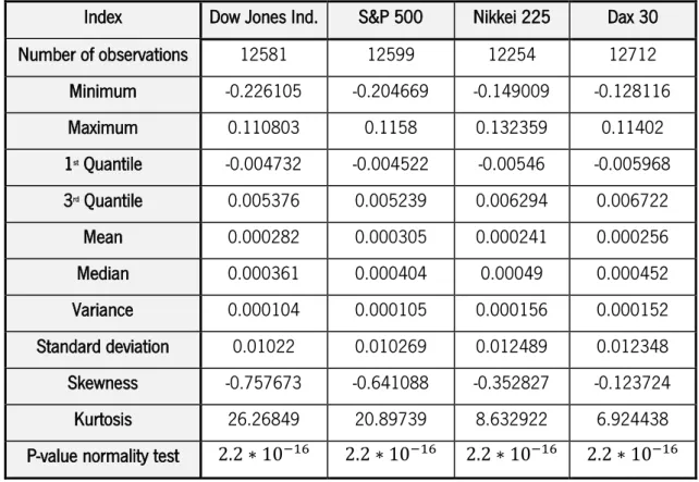
Table 1 provide basic descriptive statistics for the chosen indexes.

Index Dow Jones Ind. S&P 500 Nikkei 225 Dax 30

Number of observations 12581 12599 12254 12712 Minimum -0.226105 -0.204669 -0.149009 -0.128116 Maximum 0.110803 0.1158 0.132359 0.11402 1st Quantile -0.004732 -0.004522 -0.00546 -0.005968 3rd Quantile 0.005376 0.005239 0.006294 0.006722 Mean 0.000282 0.000305 0.000241 0.000256 Median 0.000361 0.000404 0.00049 0.000452 Variance 0.000104 0.000105 0.000156 0.000152 Standard deviation 0.01022 0.010269 0.012489 0.012348 Skewness -0.757673 -0.641088 -0.352827 -0.123724 Kurtosis 26.26849 20.89739 8.632922 6.924438

P-value normality test 2.2 ∗ 10−16 2.2 ∗ 10−16 2.2 ∗ 10−16 2.2 ∗ 10−16

Table 1: Basic stats of the four indexes.

Kurtosis provide a measure of the thickness of the tails of the distribution, the higher the value, the higher the probability of extreme events. The positive kurtosis is according to Lee & Lee & Lee

(36)

25 (2000) called leptokurtic and lower kurtosis meaning a negative excess is called platykurtic. The skewness in all indices is negative, which indicates that the returns are skewed to the left. This means another departure from the assumption of normality.

A formal normality test for each index is presented using the Jarque-Bera test. As we can observe the test rejects the hypothesis of normality for all indices.

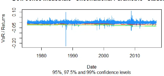
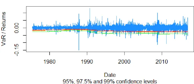
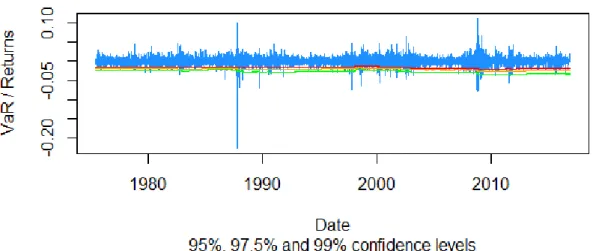
Next we can see the daily returns for each index, and in all indexes it is visible some volatility clusters, and some of the large absolute returns are visible in the graph.

Figure 2: Dow Jones Industrials daily returns from 1/1/1964 till 25/11/2016.

(37)

26

Figure 4: Nikkei 225 daily returns from 1/1/1964 till 25/11/2016.

(38)

27 5. Results

5.1 VaR calculation

With many different models and approaches possible, the choice that VaR users face is the choice of the right one that matches their purpose best. The approaches should make estimates that fit best the future distribution of returns. If an overestimation of the VaR measure is made, then investors end up with an overestimate of risk and therefore restraining their investments opportunities. On the other side, if an underestimation is made, investors may fail to cover incurred losses.

In this dissertation the VaR for the four selected indexes, being them Dow Jones Industrials, S&P 500, Nikkei 225 and Dax 30 is estimated using the Unconditional Parametric approach. The performance of the parametric approaches depends a lot on the distribution assumed for returns, so I will test different distributions as Student t, Generalized Error, Skewed Student t, Pareto and Weibull and with confidence levels of 95%, 97.5% and 99%.

The amount of data used and complexity of the calculations involved goes beyond the capabilities of more common software like Excel, so the tool that will be used to perform the calculations is the R software, through Rstudio interface.

5.1.1 Unconditional Parametric Estimation

The Unconditional Parametric approach using the maximum likelihood estimation was performed through a rolling function procedure also known as rolling window where for the Student t, Generalized Error, and Skewed Student t had a rolling window with a width of 2500 observations consisting of roughly of 10 years, while the Pareto and Weibull have a smaller one, of 1500 because this distribution can only be calculated using the days where the returns were negative. The confidence levels used were some of the most commonly used in literature and some of the recommended by Christoffersen (2012), that are 95%, 97.5% and 99%.

The figures bellow illustrate the different Unconditional Parametric VaR estimates of the different distributions assumed in comparison with the returns of each index for the several confidence levels. It is already possible to see that the Skewed Student t may be doing an underestimation of risk and the Pareto and Weibull probably may be doing an overestimation. Just by the graphs it is not possible to make further analysis neither be certain of the stated before, so in the next sections

(39)

28 empirical backtest studies are presented and will examine the models in detail and show if they can be called adequate or not.

In the next pages, the graphs with the Unconditional Parametric estimation of VaR for each index and the tree levels of confidence.

Figure 6: Dow Jones Industrials returns compared to estimated VaR for the Unconditional Parametric approach under Student t distribution from 26/06/1975 till 25/11/2016.

Figure 7: S&P 500 returns compared to estimated VaR for the Unconditional Parametric approach under Student t distribution from 26/06/1975 till 23/11/2016.

(40)

29

Figure 8: Nikkei 225 returns compared to estimated VaR for the Unconditional Parametric approach under Student t distribution from 28/08/1975 till 23/11/2016.

Figure 9: Dax 30 returns compared to estimated VaR for the Unconditional Parametric approach under Student t distribution from 18/04/1975 till 23/11/2016.

(41)

30

Dow Jones Industrials – Unconditional Parametric Generalized

Error

Figure 10: Dow Jones Industrials returns compared to estimated VaR for the Unconditional Parametric approach under Generalized Error distribution from 26/06/1975 till 23/11/2016.

Figure 11: S&P 500 returns compared to estimated VaR for the Unconditional Parametric approach under Generalized Error distribution from 26/06/1975 till 23/11/2016.

(42)

31

Figure 12: Nikkei 225 returns compared to estimated VaR for the Unconditional Parametric approach under Generalized Error distribution from 28/08/1975 till 23/11/2016.

Figure 13: Dax 30 returns compared to estimated VaR for the Unconditional Parametric approach under Generalized Error distribution from 18/04/1975 till 23/11/2016.

(43)

32

Dow Jones Industrials – Unconditional Parametric – Skewed

Student t

Figure 14: Dow Jones Industrials returns compared to estimated VaR for the Unconditional Parametric approach under Skewed Student t distribution from 26/06/1975 till 23/11/2016.

Figure 15: S&P 500 returns compared to estimated VaR for the Unconditional Parametric approach under Skewed Student t distribution from 26/06/1975 till 23/11/2016.

(44)

33

Figure 16: Nikkei 225 returns compared to estimated VaR for the Unconditional Parametric approach under Skewed Student t distribution from 28/08/1975 till 23/11/2016.

Figure 17: Dax 30 returns compared to estimated VaR for the Unconditional Parametric approach under Skewed Student t distribution from 18/04/1975 till 23/11/2016.

(45)

34

Figure 18: Dow Jones Industrials returns compared to estimated VaR for the Unconditional Parametric approach under Pareto distribution from 26/06/1975 till 23/11/2016.

Figure 19: S&P 500 returns compared to estimated VaR for the Unconditional Parametric approach under Pareto distribution from 26/06/1975 till 23/11/2016.

(46)

35

(47)

36

Figure 22: Dow Jones Industrials returns compared to estimated VaR for the Unconditional Parametric approach under Weibull distribution from 26/06/1975 till 23/11/2016.

Figure 23: S&P 500 returns compared to estimated VaR for the Unconditional Parametric approach under Weibull distribution from 26/06/1975 till 23/11/2016.

(48)

37

Figure 24: Nikkei 225 returns compared to estimated VaR for the Unconditional Parametric approach under Weibull distribution from 28/08/1975 till 23/11/2016.

Figure 25: Dax 30 returns compared to estimated VaR for the Unconditional Parametric approach under Weibull distribution from 18/04/1975 till 23/11/2016.

(49)

38 5.2 Backtests

5.2.1 Unconditional Coverage Test

As explained before the unconditional coverage test of Christoffersen (1998) accounts for the number of exceptions is more or less than the selected confidence level would indicate. In the next two pages, table 3, 4, 5 and 6 present the results of Christoffersen tests of conditional coverage for p=0,05, p=0,025 and p=0,01. The tables show the number of expected exceptions and the actual one, then the Likelihood Ratio statistic (LR) for the unconditional coverage is presented and the decision for H0: Correct number of exceptions.

(50)

39 Dow Jones Industrials

95% 97.5% 99%

Expected Actual LR test P-value Decision Expected Actual LR test P-value Decision Expected Actual LR test P-value Decision

Student t 504 535 1.962796 0.1612146 Fail to Reject H0 252 268 1.017837 0.3130327 Fail to Reject H0 100 105 0.1735459 0.6769795 Fail to Reject H0 Generalized Error 504 475 1.795397 0.18027 Fail to Reject H0 252 233 1.510538 0.219057 Fail to Reject H0 100 113 1.432854 0.2312992 Fail to Reject H0 Skewed

Student t 504 852 211.3461 0 Reject H0 252 585 330.6975 0 Reject H0 100 337 346.6681 0 Reject H0

Pareto 479 191 234.4836 0 Reject H0 239 90 125.5557 0 Reject H0 95 42 38.76329 4.784411e-10 Reject H0

Weibull 479 229 169.4076 0 Reject H0 239 121 73.54595 0 Reject H0 95 60 15.66776 7.550038e-05 Reject H0 Table 2: Unconditional Coverage Test for the Unconditional Parametric estimation of Dow Jones Industrials.

S&P 500

95% 97.5% 99%

Student t 504 588 13.68762 0.0002158732 Reject H0 252 300 8.661897 0.003249328 Reject H0 100 109 0.6255699 0.6255699 Fail to Reject H0 Generalized Error 504 580 1.31845 0.2508704 Fail to Reject H0 252 302 9.384843 0.002187867 Reject H0 100 183 54.22861 1.785239e-13 Reject H0 Skewed

Pareto 480 210 201.236 0 Reject H0 237 134 54.83506 0 Reject H0 96 50 27.07672 1.955385e-07 Reject H0

Weibull 475 252 132.1334 0 Reject H0 224 155 24.86887 1.311173e-13 Reject H0 96 67 9.310428 0.002278533 Reject H0

(51)

40 Nikkei 225

95% 97.5% 99%

Student t 487 615 32.42073 1.241552e-08 Reject H0 243 319 21.68634 3.210692e-06 Reject H0 97 142 17.94534 2.273408e-05 Reject H0 Generalized Error 487 528 3.41751 0.06450824 Fail to Reject H0 243 284 6.444848 0.01112746 Reject H0 97 150 24.47734 7.518908e-07 Reject H0 Skewed Student t 487 930 337.4565 0 Reject H0 243 644 467.6133 1.735855e-10 Reject H0 97 388 499.3622 0 Reject H0 Pareto 449 261 97.3629 0 Reject H0 224 137 40.74344 0 Reject H0 89 69 5.335423 0.02089627 Fail to Reject H0 Weibull 449 283 74.34314 0 Reject H0 242 173 22.89656 6.136537e-07 Reject H0 89 90 0.0001123171 0.9915442 Fail to Reject H0 Table 4: Unconditional Coverage Test for the Unconditional Parametric estimation of Nikkei 225.

Dax 30

95% 97.5% 99%

Student t 510 609 18.85174 1.412824e-05 Reject H0 255 338 24.97886 5.796251e-07 Reject H0 102 162 30.10444 2.273408e-05 Reject H0 Generalized

Error 510 561 5.081087 0.02418821 Reject H0 255 308 10.47827 0.001207866 Reject H0 102 170 37.97773 5.995204e-15 Reject H0

Skewed

Pareto 485 230 174.6743 0 Reject H0 242 134 59.63802 1.14353e-14 Reject H0 97 56 20.78305 5.143627e-06 Reject H0

Weibull 285 267 123.1213 0 Reject H0 242 173 22.89656 1.709574e-06 Reject H0 97 86 1.346912 0 Fail to Reject H0 Table 5: Unconditional Coverage Test for the Unconditional Parametric estimation of Dax 30.

(52)

41 As presented in table 2, the Student t and Generalized Error distribution perform best for Dow Jones Industrials, making, in terms of unconditional coverage, a fairly good estimation for all levels of confidence having a good prediction of exceptions, suggesting that they fit better the Dow Jones returns probability distribution. On the other hand, Skewed Student t made the biggest error, with exceptions being very underestimated and is therefore considered inadequate. The Pareto and Weibull distributions make similar results both with some overestimation of risk and therefore are considered inadequate for all confidence levels.

In table 3 we can see the S&P 500 results for the unconditional coverage test, and here again Student t and Generalized Error distributions performs overall best but the results are not as good as for the Dow Jones Industrials, in fact the Student t Unconditional Parametric Model is only valid for 99% VaR and for the Generalized Error one, only the 95% VaR, making both this models always an underestimation of risk. Again, as in Dow Jones Industrials, it can be seen that Skewed t distribution makes a severe underestimation of risk. Pareto and Weibull again make an overestimation of risk, and although for the p=0,01 in the Weibull distribution the gap between the predicted number of exceptions and the actual is not very big, the model is still considered inadequate.

The table 4 show the results for Nikkei 225 and it is where the Unconditional Parametric model for the Weibull distribution gets the overall result for the 99% VaR, only missing by one the exception, which, considering that this test accounts only for the unconditional coverage which alone is not enough to validate a model, is an excellent result with a Likelihood Ratio test of 0.0001123171. As for Student t, Generalized Error and Skewed Student t distributions, they all underestimate the risk, and here again the last one having the worst results overall. In Generalized Error distribution for a 90% VaR a valid model is obtained as in the previews two indexes. The Pareto and Weibull here again overestimate risk, but obtain aceptable results in the higher confidence levels (99%). For the Dax 30 index (table 5), the Unconditional Parametric approach performed worst with only one model not being rejected. The first tree distributions did as in the other indexes, an underestimation of risk with Generalized Error distribution, that although was rejected the null hypothesis still produced a Likelihood Ratio of 5.081087, in line with the previews results it is one of the best estimations in terms of conditional coverage. The Pareto and Weibull made an overestimation of risk as in all indexes, and as for Nikkei 225, the Unconditional Parametric

(53)

42 approach through the Weibull distribution provided the best result, with a valid model for the p=0,01.

5.2.2 Independence test

Failure test that examine if the number of exceptions is correct is not enough as explained before. It is also important to examine if the exceptions are spread evenly over time, or they occur in clusters. To examine this, I conduct the Christoffersen’s (2004) interval forecast test. The Null Hypothesis states: duration between exceedances have no memory. The estimated Weibull parameter b is presented as well as the result of the Null Hypothesis in the following tables.

(54)

43 Dow Jones Industrials

95% 97,50% 99%

b P-value Decision b P-value Decision b P-value Decision

Student t 0.74313 0 Reject H0 0.6309642 0 Reject H0 0.5296511 0 Reject H0

Generalized

Error 0.7294691 0 Reject H0 0.603897 0 Reject H0 0.5447902 0 Reject H0

Skewed Student

t 0.8192536 0 Reject H0 0.7424613 0 Reject H0 0.6696607 0 Reject H0

Pareto 0.5976097 0 Reject H0 0.5208795 0 Reject H0 0.4173752 0 Reject H0

Weibull 0.6269891 0 Reject H0 0.5564018 0 Reject H0 0.4620558 0 Reject H0

Table 6: Christoffersen’s (2004) Independence Test for the Unconditional Parametric estimation of Dow Jones Industrials.