Inclusion of genetic relationship information in the pedigree selection method using mixed models

Inclusion of genetic relationship information in the pedigree selection method

using mixed models

José Airton Rodrigues Nunes

, Magno Antonio Patto Ramalho

and Daniel Furtado Ferreira

Departamento de Planejamento e Política Agrícola, Centro de Ciências Agrárias,

Universidade Federal do Piauí, Teresina, PI, Brazil.

2

_{Departamento de Biologia, Universidade Federal de Lavras, Lavras, MG, Brazil.}

_{Departamento de Ciências Exatas, Universidade Federal de Lavras, Lavras, MG, Brazil.}

Abstract

We used a mixed model approach and computer simulation to evaluate the inclusion of parentage information as de-termined by the genealogy established in the pedigree method. The simulations were based on a purely additive ge-netic model for one quantitative trait of 20 unlinked segregating loci with equal effects and an allelic frequency of 0.5 for heritability values of 10%, 25%, 50% and 75% for selection based on an F4:5progeny mean. We simulated 1000 experiments for each heritability value, corresponding to the evaluation of 256 F4:5progenies. The phenotypic values of the progenies were analyzed according to two models, one ignoring and one considering the additive genetic par-entage among the progenies. The additive relationship coefficients among F4:5progenies ranged from 0.0 to 1.75. The evaluated selection procedures were the phenotypic progeny mean (M) and the best linear unbiased predictor including parentage (BLUP_A). The inclusion of parentage among progenies using theBLUP_Aprocedure resulted in higher selection gains than when the relationship information was ignored, which possibly recompenses the addi-tional work invested to obtain these records, above all in the case of low - heritability traits.

Key words:autogamous crops,BLUP, computer simulation, plant breeding. Received: February 2, 2007; Accepted: June 11, 2007.

Introduction

The pedigree method, proposed towards the end of the 19th century, is widely applied to improvement pro-grams of self-fertilized plants and is mainly based on re-cording the genealogies among progenies over the selfing generations (Ramalhoet al., 2001). However, not only is does this procedure require time and dedication from the breeder but the usefulness of this method for the selection process is somewhat restricted. One possibility of using this parentage information in support of the selection process would be in progeny evaluations in experiments with repli-cations. Such an approach could be useful since breeders of autogamous species are primarily interested in selecting progenies that, during homozygosis, accumulate a higher quantity of favorable alleles that associate the best additive genetic values (AGV), bearing in mind that the ultimate aim is the establishment of lines (Fehr, 1987). For quantitative traits, however, the phenotype does not always reflect the

associatedAGV. In this case, it would be important to use methodologies that optimize the use of the available infor-mation, in order to classify the progenies as closely as pos-sible to the ranking given by the true AGV (White and Hodge, 1989). Several fixed model and mixed model pro-cedures have been proposed to predict theAGVof proge-nies, including the best linear unbiased estimator (BLUE) method, the best linear predictor (BLP) technique and the best linear unbiased predictor (BLUP) approach (White and Hodge, 1989; Mrode, 1996; Lynch and Walsh, 1998; Re-sende, 2002).

TheBLUPprocedure has been the most widely used in the prediction of the genetic merit in animals (Mrode, 1996) and, more recently, it has been widely applied in plant improvement (Bernardo, 2002; Resende, 2002). Un-der unbalanced conditions this procedure not only has the advantage of making predictions more reliable compared to those obtained by the ordinary least square method but also incorporates information on related plants and thus optimizes the use of the available data in progeny compari-sons (Bernardo, 2002).

Since we found no reports on the use of genealogy es-tablished by the pedigree method in progeny selection in www.sbg.org.br

Send correspondence to José Airton Rodrigues Nunes. Departa-mento de PlanejaDeparta-mento e Política Agrícola, Centro de Ciências Agrárias, Universidade Federal do Piauí, Campus Socopo, Bairro Ininga, 64049-550 Teresina, PI, Brazil. E-mail: [email protected].

self-pollinated crops and field experiments produce unreli-able information (Wanget al., 2003) we evaluated the effi-ciency of selection incorporating this genetic relationship using a mixed model computer simulation.

Methodology

The program was implemented in the Delphi 6.0 en-vironment (Cantú, 2002). A simplified genetic model was assumed for any quantitative trait considering 20 loci of in-dependent segregation, with equal and additive effects and an allelic frequency of 0.5 without dominance. The simula-tions considered heritability values of 10%, 25%, 50% and 75% for selection based on an F4:5progeny mean (hp

2 ). For eachhp

2

heritability we simulated 1000 F2populations with

20 segregating loci consisting of 64 plants each. The plant multiplication rates were assumed to be equal, with each plant generated 40 offspring.

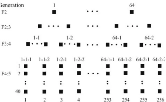
Initially, the generations were advanced by the pedi-gree method with no visual selection. A segregating F2

pop-ulation of 64 simulated plants gave rise to the 64 F2:3

progenies with 40 plants each. Two plants were randomly selected from each F2:3progeny, resulting in 128 F3:4

proge-nies and the process repeated in the following generation to finally obtain 256 F4:5progenies with 40 plants each

(Fig-ure 1).

The phenotypic values for the plants of each F4:5

progeny (yi) were simulated by adding normally distributed

random errors to the genotypic values (GV), by the follow-ing model:

yi = + +µ gi wi,

whereµis a constant (100 in the present case),giis the

genotypic effect of planti(i= 1, 2, ..., 40) andwiis the

envi-ronmental deviation associated toyi.

Thegieffect result from the cumulative effect of the

20 loci as already described in the genetic model. The addi-tive effect (al) of the lthlocus was assumed equal to 1.0,

wherel= 1, 2, ..., 20. The value ofgitaking locusBwith

two alleles (B1andB2) as reference is given by:

g a a

B B B B B B

i l l

l = = ⎧ ⎨ ⎪ ⎩⎪ =

∑

Thewieffects were randomly attributed based on a

normal distribution with constant variance,i.e.,N( ,0_σw2 ) . The variance componentσ_w2

is the environmental variance among plants, which can be obtained by:

σw σ

F F G h h 2 2 2 2 1 2 2 =⎡ − ⎣ ⎢ ⎤ ⎦ ⎥ ,

whereσG 2

is the genetic variance among the F2plants (i.e.,

σG σA σD

2 ₌ 2₊ 2

),σA 2

is the F2additive variance with, in this

case, an allelic frequency of 0.5σA l l a 2 2 1 20 2 = =

∑

was assumed equal to 1.0 for all loci, thenσA L 2

2

= / ,σD

2 is the F2variance dominance and since dominance was

as-sumed to be absent, thenσD 2

0 = , andhF2

2

is the F2generation

individual heritability.

The 40 simulated genotypes or plants per F4:5progeny

were divided into two virtual plots of 20 plants (n= 20) to produce two replications (r= 2) for each progeny. In the following equations, random errors were considered to be normally distributed among plots, withe~N( ,0 e)

2

σ in rela-tion to the mean phenotypic values of the plots. Theσe

2 vari-ance component is the environmental varivari-ance among plots.

In the simulation the relationσ / σ_w2 _e2

was considered fixed at eight (c= 8). The error terms varied according to values assumed forh_p2

heritability: h r nr p p p r d 2 2 2 2 2 = + + σ

σ σ σ

,

whereσp 2

is the genetic variance among F4:5 progenies

(σp / σA)

2 2

7 4

= ,σd

2

is the phenotypic variance within a plot (σD σGd σw

2 ₌ 2 ₊ 2

, whereσGd 2

is the genetic variance within F4:5progenies given byσGd σA

2 2

1 8

= / ). Thus the individual

F2 heritability (hF2 2

) was determined as a function of the pre-fixedhp

2

heritability values as:

h n c nr h h n c F Gd p p p Gd Gd 2 2 2 2 2 2 2 2 1 1 1 = + ⎛ ⎝ ⎜ ⎞ ⎠ ⎟ − − + ⎛_⎝ + σ σ σ σ ( ) ⎜ ⎞ ⎠ ⎟ .

We analyzed 1000 experiments corresponding to the evaluation of 256 simulated F4:5 progenies, derived from

the pedigree method. The analysis was based on the mean phenotypic data of the plots, using a completely random-ized experimental design with two replications.

According to the description of the conduction by pedigree method, each F2plant generated four F4:5

proge-nies (Figure 1). Based on this detailed pedigree, the matrix

of the additive genetic parentages among the related proge-nies was determined, considering the F2population as

non-inbred. The phenotypic progeny data were then analyzed according to two models:

ModelGI

The genetic relationship among progenies was ig-nored. The mean phenotypic data of the plots of the 256 F4:5

progenies were analyzed using a linear mixed model (Hen-dersonet al., 1959)y=Xβ+Za e+ , wherey is a 512 x 1 vector of the mean phenotypic data of the plots,Xis a 512 x 1 fixed effect design matrix,βis a scalar fixed effect of the constant,Zis a 512 x 256 random effects of progenies de-sign matrix,ais a 256 x 1 progeny random effects vector witha~N( , )0G andG= σA _a2

, whileeis a 512 x 1 vector of errors withe~N( , )0R andR= σI _e2

. TheGmatrix was des-ignated byIσ_p2

(i.e.,A= I), indicating that the progenies were assumed to be unrelated. In this case, theσ_a2

compo-nent is equal to the genetic variance among F4:5progenies

(σp 2 ).

ModelGA

In this model the genetic relationship among proge-nies was considered by the inclusion of parentage among progenies. The mixed model for analysis was identical to modelGI,except that theGmatrix was designated byAσA

2 , with A containing the additive relationship coefficients among F4:5progenies, corresponding to twice the Malecot’s

coancestry coefficient (Bernardo, 2002: section 2.3.5.2), andσ_a2

refers directly to the F2additive variance among

plants (σ_A2

). In animal breeding theAmatrix is referred to as thenumerator relationship matrix (Mrode, 1996) and, in this case, it was given by:

A=I₆₄⊗

1 75 1 50 1 00 1 00 1 50 1 75 1 00 1 00 1 00 1 00 1 75

, , , ,

, , , ,

, , , 1 50

1 00 1 00 1 50 1 75 ,

, , , ,

⎡

⎣ ⎢ ⎢ ⎢

⎤

⎦ ⎥ ⎥ ⎥,

where⊗ is the Kronecker product.

The solutions for the random (a) and fixed effects ($ β$) for both models were obtained by solving the following equation (Hendersonet al., 1959):

X X X Z

Z X Z Z A

X Z e a

′ ′

′ ′ +

⎡ ⎣⎢

⎤ ⎦⎥ ⎡ ⎣⎢

⎤ ⎦⎥=

′ ′ ⎡ ⎣

−1_$2 2 /$

$

$

σ σ β a

y

y ⎢ ⎤_⎦⎥.

To obtain the previous solutions, the components of genetic and non-genetic variances were assumed to be un-known. These variance components were estimated using the restricted maximum likelihood (REML) method (Pat-terson and Thompson, 1971). Since the REML method em-ploys an iterative process, the expectation-maximization (EM) numeric algorithm was applied (Dempster et al., 1977).

The predictions of the progeny random effects (a)$ based on the overall adjusted mixed model areBLUP pre-dictions (Henderson, 1975). After an adjustment of theGI

model the predictions were denoted asBLUPI, while for the

GA model the predictions were designatedBLUPA.

Addi-tionally, the phenotypic progeny means (M) for each simu-lated experiment were also obtained.

It should be noted that due to the balancing conditions under which the simulation were conducted and the use of an orthogonal experimental design with no missing data the

BLUPIpredictions do not have selective advantage in

rela-tion to the phenotypic means of the progenies(M) (Ken-nedy and Sorensen, 1988). Thus, only the results using the meanMwill be shown, and these should be understood as being equal toBLUPI.

For each pre-fixedhp 2

heritability, corresponding to 1000 simulated experiments, we obtained the mean esti-mates of the genetic variance among the F4:5progenies (σ$p

2 ) and heritability on an F4:5progeny mean basis (h$p

2

) for both

models (GIandGA). The selection procedures of the F4:5

progenies (meanMandBLUPA) were evaluated and

com-pared based on the true genotypic values (GV) so for both procedures we estimated the Spearman correlations (rS),

proportions of coincidence in the 5%, 10% and 25% selec-tion fracselec-tions for lower and upper extremes on the ranking of progenies, and the meanGV for different percentages (0.4% (best progeny), 5%, 10% and 25%) of the superior selected progenies.

The relative efficiency (RE) ofBLUPAin relation to

the mean M was determined by RE = {[rS(BLUPA, GV)

-rS(M, GV)]/ rS(M, GV)} x 100, whererS(BLUPA, GV)is the Spearman

correlation betweenBLUPAandGVof the selected

proge-nies, andrS(M, GV)is the Spearman correlation between the

meanMandGVof the selected progenies. The relative effi-ciency was obtained also using proportions of coincidence. We also calculated the relative gain (RG) ofBLUPAin

rela-tion to the meanM usingRG ={[MGVBLUPA - MGVM]/

MGVM} x 100, whereMGVBLUPAis the mean genotypic

val-ues of the selected progenies calculated byBLUPAwhile

MGVMis the mean genotypic values of the selected

proge-nies calculated by the meanMmethod.

Results

For both models, the mean estimates of the genetic parameters associated with the F4:5progenies were close to

the pre-fixed parametric values for all thehp 2

heritabilities studied (Table 1). Nevertheless in all the evaluations the ge-netic parameter estimates by theGAmodel, which includes

parentage among progenies, were more accurate than those produced by theGImodel. For instance, for 25%hp

2 herita-bility the standard error associated with theσ$p

2

estimate in theGAmodel was 33.5% but was 44.4% for the GImodel.

However, when 50% hp

2

model and 22.4% for the GImodel (Table 1). This

demon-strates that it is advantageous to take into account geneal-ogy (as normally occurs when using the pedigree method), although this advantage decreases as the character heritability increases (hp

2 50

≥ %).

The selection units (meanMandBLUPA) were

evalu-ated regarding the correct ranking of F4:5 progenies using

the true associated genotypic values (GV) as reference. As expected, the mean correlation estimatesrSof the evaluated

procedures were directly proportional to thehp 2

heritability values (Table 2). Thehp

2

heritability represents a determi-nation coefficient between theMandGVmeans, so that the mean values of the correlation estimates (rS(M, GV)) can be

used to verify the quality of the simulations, since they are approximate estimators of h_p2

(Falconer and Mackay,

1996). TherS(M, GV)correlation values were near the

expec-ted ( hp ) 2

values for all the hp 2

heritabilities studied

(Table 2),e.g.for 25%hp 2

heritability the meanrS(M, GV)

cor-relation estimate was 0.48 and therefore close to the popu-lation value of 0.5.

TherS(BLUPA, GV)mean correlations betweenBLUPA

andGVwere superior to therS(M,GV)mean correlation

val-ues for all the h_p2

heritability values studied (Table 2), demonstrating that the incorporation of genetic relation-ships results in greater efficiency regarding the correct classification of progenies, particularly in situations whereh_p2

heritability was less than 50%. For example, for 10%h_p2

heritability the relative efficiency (RE) ofBLUPA

to meanMwas 43.33% while for 50%h_p2

heritability the

REdropped to only 14.5%, this being confirmed by the high rS(M, BLUPA) correlation (0.87) between BLUPA and

meanM(Table 2).

The identification of the progenies in the extremes on their ranking is of greater relevance for breeders than the classification of all the progenies evaluated. For this we es-timated the coincidence proportions (C(BLUPA, GV)) of

se-lected progenies using theBLUPAand meanM methods

and compared the results with selected progenies based on the realGV(Table 3) and found that for a fixed selection fraction (s) value the corresponding proportions of

esti-mated coincidences in the lower and upper selected extremes were identical.

For allhp 2

heritability and selection fractionssvalues theC(BLUPA, GV)betweenBLUPAandGVwere higher than

theC(M, GV)between the meanMandGV, (Table 3),

support-ing ourrSestimates (Table 2). As mentioned above, theRE

of theBLUPAin relation to mean M in the coincidences

withGVwas proportionally greater for lowerhp 2

heritability values and selected fractions (s). For example, for 10%hp

2

heritability ands= 5%C(BLUPA, GV)was 0.21 andC(M, GV)

0.15 (anREof 40%), while at the samehp 2

heritability but withs= 25%REand was only 15.4%. Whenhp

2

heritability was 50%REdropped to 26.3% fors =5% and 13.3% for

s= 25% (Table 3). This indicates that the efficiency of

BLUPAcould possibly be higher when breeders work with a

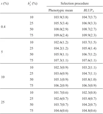
trait of low heritability and apply high selection intensity. Breeders want the selected progenies to have the highest possible genetic values, which ultimately reflect the gain achieved with selection, disregarding the progeny by environment interaction. In the selected fractions (s) com-paring theGVmeans of theBLUPA-selected progenies with

the meanMfor the pedigree method it can be seen verify

Table 1- Mean estimates of the genetic variance among F4:5progenies

(_σ$2_{p) and heritability on a F}

4:5progeny mean basis (h$p

2_{) and standard errors}

(values in brackets) according to modelGI(ignoring the pedigree

informa-tion) and modelGA(considering the pedigree information) for different

values of heritabilityhp

2 .

hp

2

(%) ModelGI ModelGA

$

σp

2 _$

hp

2

(%) σ$p

2 _$

hp

2 (%)

10 20.48(17.90) 11.12(9.22) 18.04(12.55) 10.02(6.58)

25 17.31(7.68) 24.23(9.43) 17.59(5.90) 24.78(6.85)

50 17.35(3.88) 49.25(6.96) 17.45(3.71) 49.46(6.30)

75 17.48(2.80) 74.65(3.75) 17.45(2.63) 74.72(3.60)

Table 2- Mean estimates of the Spearman correlation (rS) and standard

er-rors (in parentheses) between genotypic values (GV), phenotypic means

(M) andBLUPpredictions considering the additive parentage (BLUPA)

among F4:5progenies, conducted by the pedigree method for different

val-ues of heritability on a F4:5progeny mean basis (hp

2_).

hp

2

(%) rS(M , GV) rS(BLUPA , GV) rS(BLUPA , M)

10 0.30(0.06) 0.43(0.09) 0.69(0.04)

25 0.48(0.05) 0.62(0.06) 0.76(0.04)

50 0.69(0.04) 0.79(0.04) 0.87(0.03)

75 0.85(0.02) 0.89(0.02) 0.95(0.01)

Table 3- Mean values of the proportions of coincidences (C) and standard

errors (values in brackets) in the selection proportions (s) of 5%, 10% and

25% of the superior or inferior F4:5progenies, conducted by the pedigree

method, ranked by the parametric genotypic values (GV), phenotypic

means (M) andBLUPconsidering the additive parentage (BLUPA) for

dif-ferent values of heritability on a F4:5progeny mean basis (hp

2 ).

s(%) hp

2

(%) C(M , GV) C(BLUPA, GV) C(BLUPA, M)

5

10 0.15(0.09) 0.21(0.13) 0.40(0.11)

25 0.24(0.11) 0.33(0.14) 0.48(0.11)

50 0.38(0.12) 0.48(0.14) 0.60(0.10)

75 0.57(0.12) 0.63(0.13) 0.75(0.09)

10

10 0.22(0.07) 0.29(0.11) 0.47(0.08)

25 0.33(0.08) 0.42(0.11) 0.54(0.07)

50 0.46(0.09) 0.56(0.10) 0.66(0.07)

75 0.63(0.08) 0.69(0.08) 0.79(0.06)

25

10 0.39(0.05) 0.45(0.07) 0.60(0.05)

25 0.48(0.05) 0.56(0.06) 0.66(0.04)

50 0.60(0.05) 0.68(0.06) 0.75(0.04)

that theBLUPAprocedure offers an advantage at all thehp 2

heritabilities studied, although with lower relative gains (RG). TheRGincreased continuously ashp

2

heritability and

s decreased (Table 4), e.g., for 10% hp 2

heritability and

s= 0.4% theRGforBLUPAwas 0.77%, while fors= 25% it

was 0.59%. With higher hp

2

heritabilities RG and at

hp 2

= 50%RG= 0.65% fors= 0.4% and 0.48% fors= 25%.

Discussion

The fact that the dominance effect is not included in our genetic model does not constitute a severe restriction because the simulation involved F4:5progenies that

repre-sent only 7/64 of the dominance variance (Ramalhoet al., 2001). Furthermore, most of the characters of self-fertilized plants, including grain yield, usually show a non-expres-sive dominance effect (Souza and Ramalho, 1995; Novo-selovicet al., 2004). Van Oeveren and Stam (1992) have also verified that the dominance has little importance in computer simulations of autogamous crops.

A restriction of the simulation was the lack of visual selection, normally occurring in the pedigree method, dur-ing the conduction stages (Fehr, 1987). However, there are many literature reports on the inefficiency of visual selec-tion for characters with low (< 50%) heritability, which is the case for most characters of economic importance (Silva

et al., 1994; Cutrimet al., 1997). Thus, taking two random

plants to generate subsequent progenies probably causes no expressive effect on the results, especially forhp

2 herita-bilities lower than 50%.

It is worth mentioning that theBLUPAand meanM

estimators are phenotypic data functions that both predict additive genetic values (AGV) associated with progenies. The best estimator is therefore the one that results in the

AGVranked closest to the ranking by the trueAGV(White and Hodge, 1989). It should be noted that, with the adop-tion of theGAmodel, the predictions of the random effect of

progenies (a) or$ BLUPAcorrespond to the predictions of the

additive genetic value (AGV) of the progenies (Lynch and Walsh, 1998), indicating the theoretical superiority of the

BLUPAprocedure in relation to meanM.

An important aspect must be mentioned concerning the meaning of unbiasedness forBLUP, more specifically for BLUPA. As mentioned above, in the present context

BLUPAis a predictor of theAGVof progenies (a) derived

from the same breeding population, whose expectation, by definition, is zero [ ( )E a =0 (Falconer and Mackay, 1996).] In this context, BLUPA is unbiased in the sense that

E(a$)=E( )a (Robinson, 1991), where a$ denotes theAGV

predictors. The conclusion that can be drawn is, differently from the concept of unbiasedness for estimators of fixed ef-fects, that the unbiasedness property forBLUPdoes not re-fer to predictions of individual random effects [ (E a$)=a] but to the expected value of these effects. Summing up, whenhp

2 100

→ %,a$=E( / )a y →a, while withhp 2

0

→ we

havea$=E( / )a y →0, demonstrating that the shrinkage ef-fect in BLUPA predictions is more marked when the hp

2

values are low, resulting in lowerrS(M, BLUPA)correlation

es-timates. Thus the results of simulation showed in a concor-dant way that whenhp

2

heritability diminishes information on parentage becomes more important, so that with higher heritabilityhp

2

(> 50%) the genotypic values are already well-determined by the mean phenotypic values (M) (Duar-te and Vencovsky, 2001).

In general, our simulation showed that the inclusion of parentage among the progenies of the pedigree method using theBLUPAprocedure resulted in slightly higher

se-lections gains and more accurate estimates of genetic para-meters than when this relationship information was ignored. This possibly compensates for the additional work invested in obtaining these records, especially when inves-tigating low-heritability traits. Our results are supported by other published research showing that higher selection gains can be reached when using theG-Amodel orBLUPA

procedure (Durel et al., 1998; Bromley et al., 2000). A

study by Panter and Allen (1995) comparing twoBLUP

models (with and without the inclusion of information about genetic parentage between lines) for prediction of soybean crossings showed no marked differences between theBLUPmodels, yet the model which takes parentage into consideration performed better.

Table 4- Mean genotypic values and standard errors (values in brackets)

in the selection proportions (s) of 0.4% (best progeny), 5%, 10% and 25%

of the superior F4:5progenies, conducted by the pedigree method, ranked

by the phenotypic means (M) andBLUPconsidering the additive

parent-age (BLUPA) for different values of heritability on a F4:5progeny mean

ba-sis (hp) 2

.

s(%) hp

2

(%) Selection procedure

Phenotypic mean BLUPA

0.4

10 103.9(3.8) 104.7(3.7)

25 105.5(3.4) 106.9(3.3)

50 108.0(2.9) 108.7(2.7)

75 109.6(2.4) 109.9(2.3)

5

10 102.6(1.2) 103.7(1.5)

25 104.2(1.2) 105.4(1.4)

50 105.9(1.1) 106.7(1.2)

75 107.3(1.1) 107.6(1.1)

10

10 102.3(0.9) 103.2(1.1)

25 103.6(0.9) 104.7(1.1)

50 105.1(0.9) 105.8(1.0)

75 106.2(0.9) 106.5(0.9)

25

10 101.7(0.6) 102.3(0.8)

25 102.6(0.7) 103.4(0.7)

50 103.7(0.7) 104.2(0.7)

Acknowledgments

This research was financially supported by the Brazil-ian Agencies CAPES and CNPq. The authors gratefully acknowledge Dr. Eduardo Bearzoti for his excellent com-ments and suggestions.

References

Bernardo R (2002) Breeding for Quantitative Traits in Plants. Stemma Press, Woodbury, 359 pp.

Bromley CM, Van Vleck LD, Johnson BE and Smith OS (2000) Estimation of genetic variance in corn from F1performance with and without pedigree relationship among inbred lines. Crop Sci 40:651-655.

Cantú M (2002) Dominando o Delphi 6: A Bíblia. MAKRON Books, São Paulo, 1104 pp.

Cutrim VA, Ramalho MAP and Carvalho AM (1997) Eficiência da seleção visual na produtividade de grãos de arroz (Oryza sativaL.) irrigado. Pesq Agropeq Bras 32:601-606. Dempster A, Laird N and Rubin D (1977) Maximum likelihood

from incomplete data via the EM Algorithm. JR Stat Soc Ser B 39:1-38.

Duarte JB and Vencovsky R (2001) Estimação e predição por modelo linear misto com ênfase na ordenação de médias de tratamentos genéticos. Sci Agric 58:109-117.

Durel CE, Laurens F, Fouillet A and Lespinasse Y (1998) Utiliza-tion of pedigree informaUtiliza-tion to estimate genetic parameters from large unbalanced data sets in apple. Theor Appl Genet 96:1077-1085.

Falconer DS and Mackay TFC (1996) Introduction to Quantita-tive Genetics. 4th ed. Longman, London, 464 pp.

Fehr WR (1987) Principles of Cultivar Development: Theory and Technique. MacMillan Publishing Company, New York, 527 pp.

Henderson CR (1975) Best linear unbiased estimation and predic-tion under a selecpredic-tion model. Biometrics 31:423-447. Henderson CR, Kempthorne O, Searle SR and Von Krosigk CM

(1959) The estimation of environmental and genetic trends from records subject to culling. Biometrics 13:192-218. Kennedy BW and Sorensen DA (1988) Properties of

mixed-model methods for prediction of genetic merit under differ-ent genetic models in selected and unselected populations. In: Weir B, Goodman MM and Namkoong G (eds) Second

International Conference Quantitative Genetics. North Carolina State University, Raleigh, pp 91-103.

Lynch M and Walsh B (1998) Genetics and Analysis of Quantita-tive Traits. Sinauer Associates, Inc., Sunderland, 948 pp. Mrode RA (1996) Linear Models for the Prediction of Animal

Breeding Values. Biddles, Guildford, 184 pp.

Novoselovic D, Baric M, Drezner G, Gunjaca J and Lalic A (2004) Quantitative inheritance of some wheat plant traits. Genet Mol Biol 27:92-98.

Panter DM and Allen FL (1995) Using best linear unbiased pre-dictions to enhance breeding for yield in soybean: II Selec-tion of superior crosses from a limited number of yield trials. Crop Sci 35:405-410.

Patterson HD and Thompson R (1971) Recovery of inter-block in-formation when block sizes are unequal. Biometrika 58:545-554.

Ramalho MAP, Abreu AFB and Santos JB (2001) Melhoramento de espécies autógamas. In: Nass LL, Valois ACC, Melo IS and Inglis MCV (eds) Recursos Genéticos e Melhoramento de Plantas. Fundação MT, Rondonópolis, pp 201-230. Resende MDV (2002) Genética Biométrica e Estatística no

Me-lhoramento de Plantas Perenes. Embrapa Informação Tec-nológica, Brasília, 975 pp.

Robinson GK (1991) ThatBLUPis a good thing: The estimation of random effects. Stat Sci 6:15-51.

Silva HD, Ramalho MAP, Abreu AFB and Martins LA (1994) Efeito da seleção visual para produtividade de grãos em populações segregantes do feijoeiro. II. Seleção entre famí-lias. Cienc Prat 18:181-185.

Souza GA and Ramalho MAP (1995) Estimates of genetic and phenotypic variance of some traits of dry bean using a segre-gating population from the cross Jalo x Small White. Rev Bras Genet 18:87-91.

Van Oeveren AJ and Stam P (1992) Comparative simulation stud-ies on the effects of selection for quantitative traits in auto-gamous crop: Early selection versus single seed descent. He-redity 69:342-351.

Wang J, van Ginkel M, Podlich D, YE G, Trethowan R, Pfeiffer W, Delacy IH, Cooper M and Rajaram S (2003) Comparison of two breeding strategies by computer simulation. Crop Sci 43:1764-1773.

White TL and Hodge GR (1989) Predicting Breeding Values with Applications in Forest Tree Improvement. Kluwer Aca-demic Publishers, Dordrecht, 363 pp.