Flag algebras and tournaments
Leonardo Nagami Coregliano
Dissertation presented
to
Instituto de Matem´
atica e Estat´
ıstica
of
Universidade of S˜
ao Paulo
for
obtainment of the title
of
Master of Sciences
Program: Computer Science
Adviser: Prof. Dr. Yoshiharu Kohayakawa
During the development of this work the author received funding from Funda¸c˜ao de Amparo `a Pesquisa do Estado de S˜ao Paulo (FAPESP), grants no. 2013/23720-9 and 2014/15134-5,
and Coordena¸c˜ao de Aperfei¸coamento de Pessoal de N´ıvel Superior (CAPES). This research was partially done while the author was visiting The University of Chicago.
The author acknowledges the support of CEPID/FAPESP NeuroMat Project, Proc. 2013/07699-0 and of the FAPESP/Thematic Project Proc. 2013/03447-6.
Flag algebras and tournaments
This version of the dissertation contains the corrections and changes suggested by the Examination Committee during the defense of the original version of the work, done on 05/08/2015. A copy of the original version is
available in Instituto de Matem´atica e Estat´ıstica of Universidade of S˜ao Paulo.
Examination Committee:
• Prof. Dr. Yoshiharu Kohayakawa (president) – IME-USP
• Prof. Dr. Jie Han – IME-USP
Acknowledgements
I am grateful
to Prof. Yoshiharu Kohayakawa
for introducing me to the field of asymptotic combinatorics; and
for advising me very wisely;
to Prof. Alexander Razborov
for the hospitality while I was visiting The University of Chicago;
to Irroko Nagami
for all the love and support;
to Valdemir Aparecido Coregliano
for all the love and support;
to Stephany Mayumi Araki
for making my life even happier.
Abstract
COREGLIANO, Leonardo N. Flag algebras and tournaments. Dissertation – Insti-tuto de Matem´atica e Estat´ıstica, Universidade of S˜ao Paulo, S˜ao Paulo, 2015. Alexander A. Razborov (2007) developed the theory of flag algebras to compute the minimum asymptotic density of triangles in a graph as a function of its edge density. The theory of flag algebras, however, can be used to study the asymptotic density of several combinatorial objects.
In this dissertation, we present two original results obtained in the theory of tournaments through application of flag algebra proof techniques.
The first result concerns minimization of the asymptotic density of transitive tournaments in a sequence of tournaments, which we prove to occur if and only if the sequence is quasi-random. As a byproduct, we also obtain new quasi-random characterizations and several other flag algebra elements whose density is minimized if and only if the sequence is quasi-random.
The second result concerns a class of equivalent properties of a sequence of tournaments that we call quasi-carousel properties and that, in a similar fashion as quasi-random properties, force the sequence to converge to a specific limit homomorphism. Several quasi-carousel properties, when compared to quasi-random properties, suggest that quasi-random sequences and quasi-carousel sequences are the furthest possible from each other within the class of almost balanced sequences.
Keywords: Asymptotic combinatorics, flag algebra, tournaments, quasi-random, extremal problems.
Resumo
COREGLIANO, Leonardo N. Algebras de flags e torneios´ . Disserta¸c˜ao – Instituto de Matem´atica e Estat´ıstica, Universidade de S˜ao Paulo, S˜ao Paulo, 2015. Alexander A. Razborov (2007) desenvolveu a teoria de ´algebras de flags para calcular a densidade assint´otica m´ınima de triˆangulos em um grafo em fun¸c˜ao de sua densidade de arestas. A teoria das ´algebras de flags, contudo, pode ser usada para estudar densidades assint´oticas de diversos objetos combinat´orios.
Nesta disserta¸c˜ao, apresentamos dois resultados originais obtidos na teoria de torneios atrav´es de t´ecnicas de demonstra¸c˜ao de ´algebras de flags.
O primeiro resultado compreende a minimiza¸c˜ao da densidade assint´otica de torneios transitivos em uma sequˆencia de torneios, a qual provamos ocorrer se e somente se a sequˆencia ´e quase aleat´oria. Como subprodutos, obtemos tamb´em novas caracteriza¸c˜oes de quase aleatoriedade e diversos outros elementos da ´algebra de flags cuja densidade ´e minimizada se e somente se a sequˆencia ´e quase aleat´oria.
O segundo resultado compreende uma classe de propriedades equivalentes sobre uma sequˆencia de torneios que chamamos de propriedades quase carrossel e que, de uma forma simi-lar `as propriedades quase aleat´orias, for¸cam que a sequˆencia convirja para um homomorfismo limite espec´ıfico. V´arias propriedades quase carrossel, quando comparadas `as propriedades quase aleat´orias, sugerem que sequˆencias quase aleat´orias e sequˆencias quase carrossel est˜ao o mais distantes poss´ıvel umas das outras na classe de sequˆencias quase balanceadas.
Palavras-chave: Combinat´oria assint´otica, ´algebras de flags, torneios, quase ale-at´orio, problemas extremais.
Contents
List of symbols ix
List of figures xv
List of tables xvii
Introduction 1
1 Flag algebras 5
1.1 Scope . . . 5
1.2 Basic definitions. . . 8
1.3 Homomorphism extensions . . . 15
1.4 Interpretation homomorphisms . . . 19
1.4.1 Algebras of constants: upward operator . . . 20
1.4.2 Inductive arguments . . . 22
1.4.3 “Genuine” interpretations. . . 23
2 Minimization of transitive tournaments and quasi-randomness 25 2.1 An introduction to tournament quasi-randomness . . . 25
2.2 Minimization of transitive tournaments . . . 28
2.3 Other quasi-random properties. . . 30
2.4 Further extremal quasi-randomness properties . . . 33
3 Carousel tournaments and quasi-carouselness 41 3.1 Locally transitive tournaments . . . 41
3.2 The carousel homomorphism and the quasi-carousel properties . . . 42
3.3 Quasi-carouselness proofs. . . 45
4 Final remarks 51 A First-order logic 57 B Other topics in flag algebra 61 B.1 Semidefinite method . . . 61
viii CONTENTS
B.2 Differential method . . . 64
Bibliography 67
List of symbols
(U, I) :T1 T2 Open interpretation (U, I) of T1 inT2,19, 24, 59
(n)k =n(n−1)· · ·(n−k+ 1) Decreasing factorial, 17
<τ Order induced by the permutation τ, 7, 8
J·Kσ,η Downward operator relative toσ and η, 16–18,20, 21, 23, 28–31, 35–37,62–64, 66
[k] ={1,2, . . . , k} Set of positive integers smaller or equal tok, 7–9, 14, 16, 17,19–22, 25, 42,46, 47, 53, 58
α 1-flag onTTournament where the labelled vertex beats the unlabelled vertex, 28,31,34–38,
55, 63,64
β 1-flag on TTournament where the labelled vertex is beaten by the unlabelled vertex, 28,
34–36, 38, 55,63, 64
∼
= Isomorphic, 9, 15, 19,20, 22, 65
|F| Size of the flag F,6, 7,9, 13–17,19–21, 31, 45,48, 49, 62
δ(A) Boundary of the set A, 18
µ1 Operatorµ1, 65
∇f Gradient of function f, 65
∂1 Vertex deletion differential operator, 65, 66
φGraph,qr Quasi-random homomorphism in TGraph, 51
φPerm,qr Quasi-random homomorphism in TPerm, 51, 52
φR Carousel homomorphism, 41–46, 48, 53
φTr Transitive homomorphism, 29, 32, 33
φσ,η Extension of homomorphismφ to typeσ through η, 15,16, 18, 20, 21,23, 27–33,
36–38, 42–46,48, 55, 63, 64,66
φqr Quasi-random homomorphism,25,26, 28–34,36–38, 41, 43,44, 52, 55
x List of symbols
π(U,I) Interpretation homomorphism relative to the open interpretation (U, I),19, 20, 22,
24, 62
πF,η Interpretation homomorphism relative to the flag F through η, 22, 23,28, 29, 35–37
πF,η Interpretation homomorphism relative to the family of flags F ⊂ Fσ2
|σ2|+1 through η, 22, 23
πσ,η Upward operator relative to type extension (σ, η),20–23, 65
σ|η Type induced by η on σ, 16
τF Operation τF (see Definition 2.4.3),34–39
1σ = (σ,Id) Flag algebra unity, 9,14–18, 20–23, 27–33, 37,38, 62–64
0 Type of size 0, 9, 16,18,20, 22–39,42, 43, 45, 48,49,51, 52, 54,55,62–66
1 Type of size 1, 10, 11, 16,17, 22–24, 28,31, 35–37,55,63–66
A Type onTTournament of size 2 where the vertex labelled 1 beats the vertex labelled 2, 3, 4,
26–33, 35–38,42–48, 64
Aσ σ-flag algebra, 14–26, 28–37,42, 43, 45–48,51, 52, 54,55,61–66
Aσ
u Localization of flag algebra Aσ with respect to the multiplicative system {uℓ :ℓ ∈N},
19, 20
Aut(M) Group of automorphisms of a model M, 25,26, 35–37, 51
B(X) Set of Borel sets of the topological space X, 18
C(Fσ) Ordinary cone relative to Fσ,61–63
~
C3 3-cycle, 26–28, 31–33,48, 54, 63
~ CA
3 A-flag of size 3 whose underlying model isC~3A, 3, 4, 26–28, 30–33, 42–48, 63, 64
Csem(Fσ) Semantic cone relative to Fσ,61–63
E Type of size 2 on TGraph corresponding to an edge, 10,17, 22, 23
E Type of size 2 onTGraph corresponding to a non-edge,10, 17, 22
E Expected value,18, 23,25, 26, 28–33,36–38, 42,45,48, 55, 64
Ext(σ, η) Set of all types σ2 such that (σ2, η) is a type extension of σ, 21
F|η Restriction of flag F through η, 16, 18,20, 26, 65
List of symbols xi
Fσ,U Family of all (finite) σ-flags that are U-models up to isomorphism, 19
Fℓσ,U Family of allσ-flags up to isomorphism that are U-models and have sizeℓ, 19, 22
Fσ
ℓ Family of all σ-flags of size ℓ up to isomorphism, 9, 13–15, 17,19,22, 26, 29, 36–39,43,
46,47, 62, 63
F↓η Flag removing restriction of flag F through η, 20
G Complement of the graph G, 10, 11, 16,17, 22, 23, 51
G(~k) Blow-up of the graph G relative to vector~k, 53
Gτ Graph of inversions of permutatin τ, 8, 24
Gn,p Erd˝os–R´enyi random graph of size n and edge densityp, 1, 51
GradM ,a~ (f) Model gradient of function f relative to M~ and point a, 65, 66
Hom(Aσ,R) Set of homomorphisms from Aσ toR, 15
Hom+(Aσ,R) Set of positive homomorphisms from Aσ toR, 15–18, 20–23, 25,26, 28–37,
42,43, 45, 48, 51,52, 54, 55, 61–66
I′(F) Flag interpretation of flag F by translation I,19, 20, 22
I(M) Model interpretation of model M by translation I,19, 24, 59
IA A-flag of size 3 where the unlabelled vertex beats both labelled vertices, 3,4, 26–28,30,
32, 34–38, 43,44, 46–48
IAP Anti-parallel arc interpretation, 24
Id Identity function, 9, 14
Idk Identity permutation of sizek, 52
IInv Inversion interpretation,24
Ilink Link interpretation, 24
im Image, 9, 16,17
IOE Orientation-erasing interpretation, 24
ISOE Strict orientation-erasing interpretation, 24
Kσ Kernel of the type σ, 14, 16,20, 34, 66
Kn Complete graph on n vertices, 10, 11,15–17, 22, 23,51, 53, 58
xii List of symbols
27, 31, 32, 41,43, 45, 53–55
6σ Preorder relative to typeσ, 61–64
M Family of all finite models up to isomorphism, 66
M|W Restriction of the model M to the set W, 6, 7, 9, 14,19, 20, 66
Mσ Unique σ-flag over M,9–11, 16,17, 22, 23
Mk Family of all models of size k up to isomorphism, 6, 9,10, 51, 65
N={0,1,2, . . .} Set of natural numbers, 1–4, 6–10, 13, 15, 18,19, 25, 26, 29,31, 33, 38, 41,42, 45, 46, 48,49, 51–53, 61,62
OA A-flag of size 3 where the unlabelled vertex is beaten by both labelled vertices,3, 4,
26–30, 32, 34,35, 37, 38, 43,44, 46–48
P Probability, 9, 15, 16, 21,22, 25, 46
p(·; ·) Joint density,1–3, 6,8–10,13–15, 17, 25,26, 41, 46, 47,62, 63, 66 Pσ,η
F Probability measure extending F to σ through η,17, 18, 46,47
Pn Path on n vertices, 10, 11, 16,17, 22, 23
Pqr Set of minimization quasi-random characterizers,33,34, 37, 38
qσ,η(F) Normalizing factor of σ flag F through η,16–18
Qqr Set of quasi-randomly minimized elements, 33,34,36–38
R Field of real numbers, 14–18, 20–23,25, 26, 28–37, 42, 43, 45,48,51, 52, 54,55,61–66
R2n+1 Carousel tournament of order 2n+ 1, 4, 42,45–49, 53
R4 Tournament on 4 vertices that has a 4-cycle, 3,4,26, 27,31–33,38,42–45,48,53,55,64
Revk Reverse permutation of size k, 52
Rn,1/2 Random tournament of size n, 2,25, 26, 53
RX Set of formal R linear combinations of elements of X, 13,14, 16, 19, 34,36, 37, 66
S Family of all permutations over [k] for some k∈N, 7
S[X] Family of all permutations over the set X, 7
Sk Family of all permutations over [k], 7, 8, 10, 52
List of symbols xiii
TDigraph Theory of Digraphs,6, 24, 64
TGraph Theory of Graphs, 5, 6,10, 23, 24, 51,58, 64, 66
TGraphofinversions Theory of Graphs of Inversions, 8, 24
Tk-hypergraph Theory ofk-uniform hypergraphs, 8, 24
TPerm Theory of Permutations, 8, 10,24,51, 52, 64
TrA3 A-flag of size 3 where the unlabelled vertex is beaten by the vertex labelled 1 and
beats the vertex labelled 2, 3, 4, 26–28,30,32–39, 43,44,46–48, 64
TrW3 1-flag obtained from Tr3 by labelling the vertex with maximum outdegree, 28
TrA4 A-flag obtained from Tr4 by labelling the vertex with maximum outdegree with 1 and
the vertex with minimum outdegree with 2, 30
Trk Transitive tournament of size k,2, 3,26–34, 37,38,43–45, 48,53, 55, 63, 64
TrW2k A-flag obtained from Trk by labelling the vertex with maximum outdegree with 1 and
the vertex with second largest outdegree with 2, 28
TTournaments Theory of Tournaments, 6, 10, 24,25, 41, 45, 64
V(M) Set of vertices of the model M, 1–3,5–9, 14,16, 17, 19–21,24, 25, 35,38, 41, 42,53,
57–59,66
Var Variance, 3, 32, 33, 44
W4 Tournament on 4 vertices that has exactly one 3-cycle and one vertex with outdegree 3,
List of figures
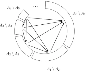
1.1 Models, types and flags in the Theory of graphs. . . 10
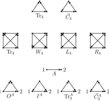
2.1 Tournaments of sizes 3 and 4, type A and A-flags of size 3. . . 27
2.2 Type 1 and flags of size 2 over the type 1. . . 28
3.1 Neighbourhoods of θ(1) andθ(2). . . 47
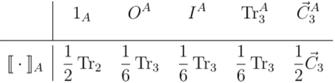
4.1 Typical structure of the random tournament SN,t. . . 54
List of tables
1.1 Joint densities in the Theory of graphs. . . 11
1.2 Joint densities in the Theory of permutations (type 0). . . 11
1.3 Joint densities in the Theory of permutations (type 1). . . 12
1.4 Downward operator in the Theory of graphs (type 1). . . 16
1.5 Downward operator in the Theory of graphs (type E). . . 17
1.6 Downward operator in the Theory of graphs (type E). . . 17
2.1 Joint densities in the Theory of tournaments (type 0).. . . 27
2.2 Downward operator in the Theory of tournaments. . . 28
3.1 Comparison of quasi-random properties and quasi-carousel properties. . . 44
Introduction
One of the most interesting measurements one can make of a large combinatorial objectN
is to compute the density of a small fixed template object M with the same signature in N (denoted by p(M;N)). Although a precise calculation of this measure requires test-ing ||VV((MN)|)| = Ω(|V(N)||V(M)|) sets, a good approximation of p(M;N) can be made by repeatedly (and independently) picking a subset of V(N) with cardinality|V(M)| uniformly at random and computing the empirical probability that this set induces an object isomorphic to M. Another good property of this measurement is its stability with respect to small changes in the large objectN, that is, ifLis obtained fromN by making changes (e.g. vertex addition or removal, predicate1 editing) that are small compared to the size2,3 |V(N)| of N,
then the density of M in L is close to the density ofM inN.
This suggests a comparison framework for large objects, or rather for sequences of objects whose sizes tend to infinity, through the density of fixed templates. More precisely, we expect that if two sequences of combinatorial objects (Nn)n∈N and (Ln)n∈N are such that
∀n∈N,|V(Nn)|=|V(Ln)|<|V(Nn+1)| lim
n→∞p(M;Nn)−p(M;Ln) = 0; for every fixed object M; then they should be very similar.
This notion of similarity of sequences of objects can be traced back to the theory of graph quasi-randomness, whose main object of study is the Erd˝os–R´enyi random graph Gn,p of
size n, in which each edge is present with probability p independently of all other edges. This theory was originated in the seminal papers by Thomason [Tho87] and Chung, Graham and Wilson [CGW89] (see also [KS06] for a survey) and its main thrust is that several a priori different properties that a sequence of graphs (Gn)n∈N of increasing sizes may have are
actually equivalent and equivalent to (Gn)n∈N being similar to the sequence of Erd˝os–R´enyi
random graphs, that is, equivalent to
lim
n→∞p(H;Gn)−p(H;G|V(Gn)|,p) = 0,
for every fixed graph H. The theory of quasi-randomness has developed into a vast field with branches in several other theories, such as uniform hypergraphs [BR13, Chu12, CG90], graph orientations [Gri13], permutations [Coo04, KP13], and tournaments [CG91,KS13].
From this notion of similarity of sequences we can also define a very useful notion of convergence, namely, we say that a sequence of combinatorial objects (Nn)n∈N of increasing
sizes is convergent if (p(M;Nn))n∈N is convergent for every fixed object M. With this notion
of convergence, one can define limit objects that codify the limits of these sequences of densities.
1
For instance, in the Theory of Graphs, edges are binary predicates.
2
In classical combinatorics, we usually call |V(N)| the order of N, but here we choose to use size in conformity with flag algebra nomenclature.
3
Or rather, in the case ofk-ary predicate editing, compared to|V(N)|k
.
2 Introduction
One approach is to define the limit objects to be semantically close to the underlying combinatorial objects, that is, to find a limit object that resembles some representation of the combinatorial objects (such approach was first taken by Lov´asz and Szegedy by defining graphons [LS06] and has also been taken in the definitions of hypergraphons [ES12], permutons [HKM+13], and digraphons [DJ08, Section 9]). The clear advantage of this approach is that operations and proofs involving these limit objects have intuitive analogous versions in the finite world.
Another approach is to study the convergent sequences syntactically, that is, to study what kind of properties the sequence of numbers (φ(M))M must satisfy if we have φ(M) =
limn→∞p(M;Nn). This latter approach is precisely the thrust of the theory of flag
alge-bras [Raz07], whose main advantages are its generality — in the sense that it constructs the limit object of any universal theory T — and the simplicity of the arguments in its proofs4.
A first and trivial observation about this sequence (φ(M))M = (limn→∞p(M;Nn))M is
that each of its coordinates is a number in the interval [0,1]. Taking this one step ahead, we see that actually some coordinates are limited to an even smaller set; for instance, in the Theory of Tournaments, if T is a sufficiently large tournament, then it cannot be that no triple of vertices induces a transitive tournament5. A natural problem that arises is then the
following.
Problem. Given a fixed object L, what is the minimum and the maximum value of φ(L) subject to (φ(M))M = (limn→∞p(M;Nn))M for a sequence of objects (Nn)n∈N of increasing
sizes?
Furthermore, if (Nn)n∈N is a sequence of objects of increasing sizes that attains this
minimum (or maximum), then what does this sequence look like?
This translates into the following classical extremal combinatorics problem.
Problem. Given a fixed object M, compute the following extremal values.
inf {lim inf
n→∞ p(M;Nn) : (Nn)n∈N is a sequence of objects with nlim→∞|V(Nn)|=∞}; sup{lim sup
n→∞
p(M;Nn) : (Nn)n∈N is a sequence of objects with lim
n→∞|V(Nn)|=∞}. Furthermore, if (Nn)n∈N is an extremal sequence, that is, if limn→∞p(M;Nn) equals the
infimum (or supremum) above, then what does Nn look like?
Going back to our tournament example, since the transitive tournament Trk of size k has
a very organized structure, a natural guess for an extremal sequence for the minimization problem would be the sequence of random tournaments (Rn,1/2)n∈N, where Rn,1/2 is the
random tournament of sizen in which each arc orientation has probability 1/2 independently of other pairs of vertices.
The first original result of this dissertation (Theorem 2.2.2), obtained in joint work with Alexander A. Razborov, says that not only does the sequence (Rn,1/2)n∈N minimize the
density of the transitive tournament of size k, but also it is the only minimizer fork >4 in the following sense: if (Tn)n∈N is a sequence of tournaments of increasing sizes minimizing
the density of Trk, then (Tn)n∈N is quasi-random, that is, we have
lim
n→∞p(T;Tn)−p(T;R|V(Tn)|,1/2) = 0, for every fixed tournamentT.
4
Perhaps only once you get used to its notation.
5
Introduction 3
With the same proof techniques, we also generalize this result to several formal linear combinations of tournaments (Theorem 2.4.9), that is, we obtain several otherPiciLi such
that (Tn)n∈N minimizes
lim
n→∞p
X
i
ciLi;Tn
!
= lim
n→∞
X
i
cip(Li;Tn)
if and only if (Tn)n∈N is quasi-random.
Perhaps two of the most interesting quasi-random properties concern what we call in the language of flag algebras A-flag density concentration. Given an arc uv ∈ A(T) of a tournament T, all other vertices w∈V(T) can be classified into four classes (“A-flags”):
• uw, vw∈A(T);
• wu, wv ∈A(T);
• uw, wv ∈A(T);
• wu, vw∈A(T). Let OA(u, v), IA(u, v), TrA
3(u, v) and C~3A(u, v) denote the number of vertices in these four classes divided by |V(T)| −2 respectively. One keystone quasi-random property (P4, to be
exact) says that a sequence of tournaments (Tn)n∈N is quasi-random if and only if
lim
n→∞O
A(u
n,vn) = 1/4 a.s.,
where unvn is an arc ofTn chosen uniformly at random. By flipping all arcs, it is easy to see
that an analogous property with IA is also a quasi-random property.
As a byproduct of the first result we are able to prove (Theorem 2.3.1) that the two other analogous properties (concerning TrA3 and C~A
3 ) are also quasi-random properties. In fact, we can even get rid of the 1/4 in the first three classes, that is, we prove (Theorem2.3.6) that if F ∈ {OA, IA,TrA
3}, then the property lim
n→∞Var[F(un,vn)] = 0
is a quasi-random property. For the final class, we prove (Theorem2.3.7) that if
lim
n→∞Var[
~
C3A(un,vn)] = 0,
then the sequence (Tn)n∈N either is quasi-random or is similar to the sequence of transitive
tournaments6 (Tr
n)n∈N.
Noting that the result on minimization of transitive tournaments closes the non-trivial cases of minimization of a single tournament (Corollary 2.2.5), we shift our attention to the maximization problem in the Theory of Tournaments.
The second original result of this dissertation concerns maximization of the tournamentR4 (which is the only tournament on 4 vertices containing a 4-cycle) and what we call
quasi-carousel properties.
As one may imagine, the quasi-carousel properties are a set of a priori different prop-erties that a sequence of tournaments (Tn)n∈N of increasing sizes may have and that are
6
4 Introduction
actually equivalent and equivalent to (Tn)n∈N being similar to a certain sequence of
tourna-ments (R2n+1)n∈N (we call the tournaments of this sequence carousel tournaments).
One of the quasi-carousel properties is the maximization of the density of R4 and we also present several quasi-carousel properties that have nice analogies in quasi-randomness. For instance, the quasi-carousel properties analogous to the A-flag concentration in quasi-randomness are the following: if F is one of OA, IA, TrA
3 or C~3A, then quasi-carousel Property S5(F,1/2) of a sequence of tournaments (Tn)n∈N says that if unvn is an arc of Tn
chosen uniformly at random, then F(un,vn) converges in distribution to a uniform random
variable on [0,1/2].
Chapter 1
Flag algebras
The aim of this chapter is to introduce the reader to the theory of flag algebras developed by Razborov [Raz07] and in doing so we choose to take an intuitive approach rather than a more formal one. Throughout this text we will follow the notation of [Raz07] so the accustomed reader is free to skip this chapter. We remark that we do not follow the order of [Raz07] when presenting the concepts and properties of flag algebras1. This chapter also
assumes the reader to be familiar with basic notions of first-order logic (we provide, however, some definitions and properties on the matter in Appendix A and every first appearance of these terms on the text will methodically be in an emphasized font).
Finally, we refer the reader to [Raz13b] for a shorter and (even more) intuitive introduction to the theory of flag algebras and to [Raz13a] for a survey of results using this theory.
1.1
Scope
The theory of flag algebras can be applied to any combinatorial structure that can be described by a universal theory in a finite first-order language with equality and without
constant or function symbols. Its main goal is to study densities of a combinatorial object in another (much larger) combinatorial object. In this section, we define the notion of density in an arbitrary universal theory and present some typical combinatorial structures that can be formulated as universal theories. We also present some basic properties regarding first-order formulations.
We start with three classic examples of combinatorial structures and their first-order formulations.
Example 1.1.1. TheTheory of GraphsTGraph can be formulated in alanguagewith a binary
predicate symbol e that codifies adjacency between two vertices, i.e., if v and w are two vertices of a graph G (that is, two elements of the set of vertices V(G) of the model G
of TGraph), then vw is an edge of G if and only ifG|=e(v, w). The axiomsof TGraph are the following.
i. ∀x,¬e(x, x);
ii. ∀x∀y,(e(x, y) =⇒e(y, x)).
If G is a model of TGraph, that is, ifG is a graph, then the set of edges of G is E(G) =
{{v, w} ⊂V(G) :G|=e(v, w)}.
1
But we attempt to provide references specific to the level of sections and theorems so the interested reader can easily find them in [Raz07].
6 Flag algebras
Note that axiom (i)enforces that the graphs do not have loops and axiom(ii)enforces the symmetry of the adjacency relation. By removing the symmetry axiom, we obtain the Theory of Digraphs below.
Example 1.1.2. The Theory of Digraphs TDigraph can be formulated in a language with a binary predicate symbol a where, if v andw are two vertices of the digraph D, then vw is an arc of D if and only ifD |=a(v, w). The theoryTDigraph has only the following axiom.
i. ∀x,¬a(x, x).
If D is a model ofTDigraph, that is, if D is a digraph, then the set of arcs of Dis A(D) =
{(v, w)∈V(D)2 :D|=a(v, w)}.
The Theory of Digraphs can be further restricted to obtain the Theory of Tournaments, i.e., the theory of digraphsDsuch that for every pair of distinct verticesv, w∈V(D), exactly one arcvw or wv is in A(D).
Example 1.1.3. The Theory of Tournaments TTournaments can be formulated in a language with a binary predicate symbola with the following axioms.
i. ∀x,¬a(x, x);
ii. ∀x∀y,(x6=y=⇒a(x, y)⊻a(y, x)).
Let us fix until the end of this chapter a universal theory T in a finite first-order language {=} ∪L with equality = and without constant or function symbols. Let us also assume that T has at least one infinite model. In fact, from here onward, unless explicitly said otherwise, all universal theories will be in a finite first-order language with equality and without constant or function symbols. Whenever we work with more than one theory, we shall append [T] to the notation accordingly to avoid ambiguity.
Note that the fact that T is universal without constant or function symbols implies that if M |= T and W ⊂ V(M), then the model restriction M|W of M to W is a model of T,
called model induced byW inM (see PropositionA.4).
This along with the existence of an infinite model of T implies that T has at least one model of each finitesize. Let us denote the size of a model M by |M|= |V(M)|, denote the family of all models of size k up to isomorphism by Mk and denote the family of all finite
models up to isomorphism by M=Sk∈NMk.
With the notion of model restriction, we can easily define the notions of submodel and submodel density below.
Definition 1.1.4. LetM and N be models of T.
An occurrence of M in N is a setW ⊂V(N) with |W|=|M| such thatN|W ∼=M.
If |M| 6|N| <∞, then we define the submodel density (or density) ofM in N as the number of occurrences of M in N divided by ||MN||, and we denote it by p(M;N).
If there exists an occurrence of M in N, then we say thatM is a submodel of N.
Remark 1.1.5. The quantity p(M;N) can be seen as the probability that a random subset of V(N)of size |M| is an occurrence of M inN.
We also remark that the notion of submodel corresponds to the notions of induced subgraph, induced subdigraph and (induced) subtournament in the theories TGraph, TDigraph and TTournaments respectively.
Note that the fact that every model restriction of a model is also a model implies that
X
M∈Mk
Scope 7
for every k 6|N|.
Another typical example of universal theory is obtained by forbidding a family of finite submodels from another universal theory.
Example 1.1.6. Let F be a family of finite models ofT. The theory of the models M of T
such that no member of F is a submodel of M can be formulated as a universal theory by appending toT the axiom
∀x1∀x2· · · ∀xk¬φN,
for each N ∈ F, whereφN is an open diagram of N overx1, x2, . . . , xk (and k =|N|).
The next proposition gives us an easier characterization of combinatorial structures that can be formulated as universal theories.
Proposition 1.1.7. Suppose T′ is a theory in a finite first-order language L and suppose that for every model M of T′ and every W ⊂V(M), the model restriction M|
W is a model
of T′. Then T′ can be reformulated as a universal theory, that is, there exists a universal theory T over Lsuch that for every model M overL, we have M |=T ⇐⇒M |=T′.
Proof. Let F be the family of all finite models overL that are not models ofT′ and consider the theory T overL whose axioms are of the form
∀x1∀x2· · · ∀xk¬φM,
for M ∈ F and where φM is an open diagram of M overx1, x2, . . . , xk.
Trivially T is universal and every model of T is a model of T′.
On the other hand, if M is a model of T′, then every model restriction of M is also a model of T′, hence not an element of F. Therefore M must also be a model of T. Remark 1.1.8. Informally, Proposition 1.1.7 says that a theoryT is universal if and only if every model restriction of T is a model of T.
Note, however, that the formulation of T given in Proposition 1.1.7 is not necessarily effective (in the sense that its axioms can be recursively enumerated), but this is not important for us here.
Perhaps the first non-trivial example of combinatorial structure that can be formulated as a universal theory is the Theory of Permutations below.
Example 1.1.9. A permutation over a setX is a bijective function τ: X →X. We denote the set of all permutations over X byS[X].
We are particularly interested in the case whenX = [k] ={1,2, . . . , k}, so we defineSk = S[[k]]. We also define S=S
k∈NSk.
Every permutation τ ∈ Sk induces an order <τ over [k] called order induced by the
permutation τ and defined by
i <τ j ⇐⇒τ(i)< τ(j),
for every i, j ∈[k].
If τ ∈Sk and η ∈ Sm, then an occurrence of τ in η is a set S = {s1, s2, . . . , sk} ⊂ [m] with s1 < s2 <· · ·< sk such that for every i, j ∈[k], we have
i <τ j ⇐⇒si <η sj.
8 Flag algebras
The Theory of Permutations (over [k] for some k ∈ N) TPerm can be formulated in a language with two binary predicate symbols a and b both with the axioms of total order, that is, we have the following axioms.
i. ∀x∀y, a(x, y)∨a(y, x);
ii. ∀x∀y,(a(x, y)∧a(y, x) =⇒x=y); iii. ∀x∀y∀z,(a(x, y)∧a(y, z) =⇒a(x, z)); iv. ∀x∀y, b(x, y)∨b(y, x);
v. ∀x∀y,(b(x, y)∧b(y, x) =⇒x=y); vi. ∀x∀y∀z,(b(x, y)∧b(y, z) =⇒b(x, z)).
Every permutationτ ∈Skcorresponds to the model over[k]whereaandbare respectively interpreted as the natural order <over [k] and the order<τ. The notions of occurrence and
density of Definition 1.1.4coincide with the ones defined in this example.
Now we present a non-trivial example of a theory which can be easily seen to be universal in light of Proposition 1.1.7.
Example 1.1.10. Thegraph of inversionsof a permutationτ ∈Sk, denoted byGτ, is given by
V(Gτ) = [k];
E(Gτ) ={{i, j} ⊂[k] :i < j∧j <τ i}.
The Theory of Graphs of Inversions is denoted by TGraphofinversions.
Clearly any induced subgraph of a graph of inversions (of some permutation) is a graph of inversions (of some permutation), henceTGraphofinversions can be formulated as a universal theory.
Finally, let us present a theory with a predicate of higher arity.
Example 1.1.11. The Theory of k-uniform hypergraphs Tk-hypergraph can be formulated in a language with a k-ary predicate symbol e where, if v1, v2, . . . , vk are vertices of the
hypergraph H, then v1v2· · ·vk is a hyperedge of H if and only if H |=e(v1, v2, . . . , vk). The
axioms of Tk-hypergraph are the following.
i. ∀x1∀x2· · · ∀xk−1,¬e(x1, x1, x2, x3, . . . , xk−1); ii. ∀x1∀x2· · · ∀xk, Vσ∈Ske(xσ(1), xσ(2), . . . , xσ(k))
⊻ Vσ∈S
k¬e(xσ(1), xσ(2), . . . , xσ(k))
.
If H is a model ofTk-hypergraph, that is, if H is a k-uniform hypergraph, then the set of hyperedges of H is
E(H) = {W ={w1, w2, . . . , wk} ⊂V(H) :H |=e(w1, w2, . . . , wk)}.
1.2
Basic definitions
Basic definitions 9
about these quantities, we often need to analyse a more general notion of density in which some vertices of M must be mapped to some prescribed values inV(N). To make this notion more precise, we first need some definitions.
Definition 1.2.1([Raz07, Section 2.1]).A type in the universal theory T is a model σ of T
such that V(σ) = [k], for some k∈N (k =|σ|).
Let σ be a type of size k. We extend the language L to L(c1, c2, . . . , ck) by appending
new constant symbols c1, c2, . . . , ck and define the extension of the theory T by the type σ as
the universal theory Tσ over the languageL(c
1, c2, . . . , ck)obtained by appending the open
diagram of σ over c1, c2, . . . , ck to the axioms of T.
We also define a σ-flag as a finite model M ofT partially labelled with [k]in a way that the labelling is a model embedding of σ in M. Formally, aσ-flag is a pair(M, θ)such thatM
is a finite model of T and θ: [k]→V(M)is a model embedding of σ inM. The size of the σ-flag F = (M, θ)is defined as |F|=|M|.
Note that there exists a unique type of size 0 and it will be denoted by 0 for convenience. Note also that a σ-flag can be alternatively seen as a finite model of the theoryTσ and
as such we borrow some notation and nomenclature from this theory.
Definition 1.2.2 ([Raz07, Section 2.1]). If σ is a type of size k, we will often denote aσ-flag F = (M, θ)by explicitly listing the values of θ in the form (M, θ(1), θ(2), . . . , θ(k)). If F = (M, θ) and F′ = (M′, θ′) are σ-flags, we define a flag embedding of F in F′ as a model embedding α of Tσ, that is, the function α: V(M)→V(M′) is a model embedding of T such that α◦θ = θ′ (i.e., it preserves labelling). Furthermore, we say that F and F′ are isomorphic(denoted by F ∼=F′) if they are isomorphic as models ofTσ, that is, if there
exists a bijective flag embedding ofF inF′.
Note that if F = (M, θ) is a σ-flag and W ⊂V(M) is such that the image im(θ) ofθ is contained in W, then F|W = (M|W, θ) is also a model of Tσ, i.e., a σ-flag.
Let us denote the family of all σ-flags of size ℓ up to isomorphism by Fσ
ℓ and denote the
family of all (finite) σ-flags up to isomorphism byFσ.
Note that Mℓ can be naturally identified with Fℓ0. Furthermore, note that F|σσ| has exactly one element, which will be denoted by 1σ and is given by 1σ = (σ,Id), where Id is
the identity automorphism of σ.
When there exists a model embedding of a type σ in a model M and all σ-flags resulting from such model embeddings are isomorphic, we will denote such σ-flag by Mσ.
We are now in condition of defining the more general notion of density calledjoint density.
Definition 1.2.3 ([Raz07, Definition 1]). Let σ be a type of size k, let ℓ, ℓ1, ℓ2, . . . , ℓt > k
be integers such that
t
X
i=1
ℓi
!
−(t−1)k 6ℓ, (1.1)
and letF = (M, θ), F1, F2, . . . , Ft∈ Fσ be σ-flags of sizes ℓ, ℓ1, ℓ2, . . . , ℓt respectively.
Thejoint densityofF1, F2, . . . , Ftin the flag F (denoted byp(F1, F2, . . . , Ft;F)) is defined
through the following random experiment. We pick uniformly at random pairwise disjoint subsets W1,W2, . . . ,Wt of V(F)\im(θ) subject to |Wi|= ℓi −k for every i∈ [t] (whose
existence is guaranteed by inequality (1.1)) and set
10 Flag algebras
Furthermore, if F1, F2 ∈ Fσ are σ-flags such that p(F1;F2)>0, then we say that F1 is a subflag of F2.
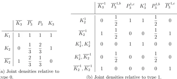
Throughout this chapter, we will mainly use as examples the theories TGraph and TPerm. A third example with TTournaments can be found in Chapter 2(see Definitions 2.1.3 and 2.2.1). Example 1.2.4. In the Theory of GraphsTGraph(see Figure1.1), for everyℓ∈N, letKℓ, Pℓ ∈
Mℓ denote respectively the complete graph on ℓ vertices and the path on ℓ vertices (i.e., of
lengthℓ−1). Furthermore, for every graph G, let G denote the complement ofG.
1 1 2 1 2 1 1
K1 1 K2 K2 E E K21 K21
K3 P3 P3 K3
1 1 1 1 1 1
K3 1
P3
1,b P1,c
3 K
1
3 P31,b P31,c
1 2 1 2 1 2 1 2
P3
E
P3E,c KE
3 P3E,b
1 2 1 2 1 2 1 2
K3
E
P3
E,b
P3
E,c PE
3
Figure 1.1: Models, types and flags in the Theory of graphs.
Let 1 denote the unique type of size 1 and let E and E denote the types of size 2 corresponding respectively to the edge and the non-edge.
With our previously defined notation ofMσ for a modelM and a typeσ, we have already
defined the1-flags K1
ℓ and Kℓ
1
, the E-flag KE
ℓ ; and the E-flag Kℓ E
. Note, however, that the notation Mσ cannot be used for P
3 and E neither forP3 andE. For these cases, we will append b or c to the superscript to distinguish between the non-isomorphic flags.
Figure 1.1 includes definitions of more flags in TGraph and Table 1.1 includes several examples of joint densities in this theory.
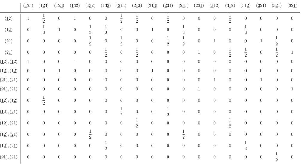
Example 1.2.5. In the Theory of Permutations TPerm, we denote a permutation τ ∈Sn by listing its image as (τ(1)τ(2)· · ·τ(n)). We also denote the unique type of size 1 in TPerm by 1. Finally, we denote a 1-flag in this theory by underlining the labelled vertex of the permutation, e.g., we denote by (312) the 1-flag over the model τ = (312) with label on vertex τ(3) = 2.
Basic definitions 11
K3 P3 P3 K3
K1 1 1 1 1
K2 0 1 3
2
3 1
K2 1 2 3
1
3 0
(a) Joint densities relative to type 0.
K3 1
P3 1,b
P31,c K31 P31,b P3 1,c
K21 0 1
2 1 1
1
2 0
K2 1
1 1
2 0 0
1
2 1
K21, K21 0 0 1 1 0 0
K21, K2 1
0 1
2 0 0
1
2 0
K2 1
, K2 1
1 0 0 0 0 1
(b) Joint densities relative to type 1.
Table 1.1: Joint densities in the Theory of graphs p(A;B), where A is given by the leftmost entry of the line and B by the topmost entry of the column.
(123) (132) (213) (231) (312) (321)
(1) 1 1 1 1 1 1
(12) 1 2
3 2 3 1 3 1 3 0
(21) 0 1
3 1 3 2 3 2 3 1
12 F lag al ge b ras
(123) (123) (123) (132) (132) (132) (213) (213) (213) (231) (231) (231) (312) (312) (312) (321) (321) (321)
(12) 1 1
2 0 1 0 0
1 2
1
2 0
1
2 0 0 0
1
2 0 0 0 0
(12) 0 1
2 1 0
1 2
1
2 0 0 1 0
1
2 0 0 0
1
2 0 0 0
(21) 0 0 0 0 1
2 0
1
2 0 0
1 2
1
2 0 1 0 0 1
1
2 0
(21) 0 0 0 0 0 1
2 0
1
2 0 0 0 1 0
1 2 1 2 0 1 2 1
(12),(12) 1 0 0 1 0 0 0 0 0 0 0 0 0 0 0 0 0 0
(12),(12) 0 0 1 0 0 0 0 0 1 0 0 0 0 0 0 0 0 0
(21),(21) 0 0 0 0 0 0 0 0 0 0 0 0 1 0 0 1 0 0
(21),(21) 0 0 0 0 0 0 0 0 0 0 0 1 0 0 0 0 0 1
(12),(12) 0 1
2 0 0 0 0 0 0 0 0 0 0 0 0 0 0 0 0
(12),(21) 0 0 0 0 0 0 1
2 0 0
1
2 0 0 0 0 0 0 0 0
(12),(21) 0 0 0 0 0 0 0 1
2 0 0 0 0 0
1
2 0 0 0 0
(12),(21) 0 0 0 0 1
2 0 0 0 0 0
1
2 0 0 0 0 0 0 0
(12),(21) 0 0 0 0 0 1
2 0 0 0 0 0 0 0 0
1
2 0 0 0
(21),(21) 0 0 0 0 0 0 0 0 0 0 0 0 0 0 0 0 1
2 0
Basic definitions 13
The following two basic properties of joint density provide motivation for the flag algebra definitions to come.
Lemma 1.2.6 ([Raz07, Lemma 2.2]).Let σ be a type of size k, let ℓ,ℓ, ℓe 1, ℓ2, . . . , ℓt>k be
integers such that
t
X
i=1
ℓi
!
−(t−1)k6ℓe6ℓ.
and letF, F1, F2, . . . , Ft ∈ Fσ beσ-flags of sizes ℓ, ℓ1, ℓ2, . . . , ℓt respectively.
Under these circumstances, we have
p(F1, F2, . . . , Ft;F) =
X
e
F∈Fσ
e
ℓ
p(F1, F2, . . . , Ft;Fe)p(Fe;F).
Lemma 1.2.7 ([Raz07, Lemma 2.3]). Under the same circumstances of Lemma 1.2.6, we have
p(F1, F2, . . . , Ft;F)−
t
Y
i=1
p(Fi;F)
6 C ℓ ,
for some constant C that depends only on ℓ1, ℓ2, . . . , ℓt, but not onℓ.
Recall that we are interested in studying densities of small objects in large objects. This provides a motivation for the following definitions.
Definition 1.2.8([Raz07, Definition 7]).A sequence ofσ-flags(Fn)n∈Nisincreasingif|Fn|<
|Fn+1| for every n∈N.
A sequence of σ-flags (Fn)n∈N isconvergent if it is increasing and (p(F;Fn))n∈N is
conver-gent for everyσ-flag F ∈ Fσ.
Note that if F ∈ Fσ is a σ-flag then we can think of the functional p(· ;F) as an
elementv of the compact metric space [0,1]Fσ
, where the coordinateF′ of v is p(F′;F), for every F′ ∈ Fσ. The next lemma follows by compactness of [0,1]Fσ
.
Lemma 1.2.9([Raz07, Theorem 3.2]). Every increasing sequence ofσ-flags has a convergent subsequence.
Let us now provide some intuition of the definitions that will come. Suppose that (Fn)n∈N
is a convergent sequence ofσ-flags and letφ: Fσ →Rbe defined byφ(F) = lim
n→∞p(F;Fn).
Note that Lemma1.2.6with t= 1 implies that, for everyF ∈ Fσ
ℓ of sizeℓ and everyℓe>ℓ,
we have
φ(F) = X e
F∈Fσ
e
ℓ
p(F;Fe)φ(Fe).
This suggests that we should think of φ not as a function with domain Fσ, but rather with
domain being a quotient of the set RFσ of formal linear combinations of σ-flags by relations given by Lemma 1.2.6.
Furthermore, if F1 andF2 areσ-flags of sizes ℓ1 andℓ2 respectively and eℓ>ℓ1+ℓ2− |σ|, then Lemma 1.2.6with t = 2 together with Lemma 1.2.7 says that
φ(F1)φ(F2) =
X
e
F∈Fσ
e
ℓ
14 Flag algebras
This provides intuition to define a product in the domain of the function φ that should be preserved by such functions obtained as limits of convergent sequences.
But before doing so, let us define the notion of a non-degenerate type.
Definition 1.2.10 ([Raz07, Definition 2]).A type σ is non-degenerate if for every ℓ> |σ|, we have Fσ
ℓ 6=∅. Alternatively, the type is non-degenerate if Tσ has an infinite model.
For completeness, we call a type σ degenerateif it is not non-degenerate.
Proposition 1.2.11 ([Raz07, Lemma 2.4]).Let σ be a non-degenerate type of size k and let Aσ =RFσ/Kσ denote the quotient of the set RFσ of formal R-linear combinations of
elements ofFσ by the linear subspace Kσ generated by elements of the form
F − X e
F∈Fσ
e
ℓ
p(F;Fe)F ,e
whereℓe>|F|.
Under these conditions, the product · : Fσ × Fσ → Aσ defined by
F1·F2 =
X
F∈Fσ ℓ
p(F1, F2;F)F,
for all flags F1, F2 ∈ Fσ and everyℓ >|F1|+|F2| −k is well-defined.
Furthermore, the (bi)linear extension of this product to RFσ×RFσ induces a product inAσ, that is, for every f ∈ Aσ and everyg ∈ Kσ, we have f ·g, g·f ∈ Kσ.
Moreover, equipping Aσ with this product (and with the usual addition) makes it a
commutative associative R-algebra with unity 1σ = (σ,Id) calledσ-flag algebra.
In usual theories, all types are non-degenerate. We provide, however, the following straightforward lemma to remove non-degenerate types from any universal theory.
Lemma 1.2.12.If T is a universal theory, then the theory of all models of T that are not isomorphic to any degenerate type ofT can be formulated as a universal theory.
Proof. TakeF as the family of all degenerate types and do as in Example 1.1.6. One could think that by removing all non-degenerate types, we could end up with a theory without any model, but the following lemma says that this is not the case since T has at least one infinite model.
Lemma 1.2.13. IfT has one infinite model M, thenM is a model of the theoryT′ obtained through Lemma 1.2.12.
Proof. It is enough to prove that there does not exist a degenerate typeσ that is a submodel of M. But this is trivially true, because if W ⊂V(M) is such that there exists an isomor-phismθ betweenσ andM|W, then for every ℓ>|σ|, taking a set X ⊂V(M) with |X|=ℓ
and W ⊂X yields (X, θ)∈ Fσ
ℓ, hence σ is non-degenerate, a contradiction.
Let us finally provide a standard example of a degenerate type.
Example 1.2.14. Let σ be a type of a theory T of size k and φ be the open diagram of σ. Let also n > k be an integer and consider the theoryT′ obtained from T by appending the axiom
∀x1∀x2· · · ∀xn,
^
i1,i2,...,ik∈[n]
Homomorphism extensions 15
Since n > k, the type σ is also a type of T′. However, it is a degenerate type of T′ since Fσ
m =∅for every m >n.
Furthermore, if M is an infinite model ofT that has no occurrence of σ, thenM is also an infinite model of T.
For instance, in the theory of graphs such that every four distinct vertices are triangle-free, the type corresponding to the triangle K3 is degenerate.
Now that we have an R-algebra, one of the most natural sets to study is the set of homomorphisms from it to the field R.
Definition 1.2.15 ([Raz07, Definition 5]).Let σ be a non-degenerate type. We denote the set of R-algebra homomorphismsfrom Aσ to R byHom(Aσ,R).
Furthermore, we define the set of positive homomorphisms fromAσ toR as the set
Hom+(Aσ,R) = {φ ∈Hom(Aσ,R) :∀F ∈ Fσ, φ(F)>0}.
Finally, let (Fn)n∈N be a convergent sequence of flags and φ ∈ Hom+(Aσ,R). We say
that (Fn)n∈N converges to φ or thatφ is the limit of the sequence(Fn)n∈N if
lim
n→∞p(F;Fn) =φ(F), for every fixedσ-flag F ∈ Fσ.
Remark 1.2.16. Since there will be no use for non-positive homomorphisms in this text, we will abuse terminology by calling a positive homomorphism just a homomorphism.
Remark 1.2.17.Note that if φ ∈ Hom+(Aσ,R), then we actually have φ(F) ∈ [0,1] for
every F ∈ Fσ.
This follows from φ(1σ) = 1 and the fact that PF∈Fσ
ℓ F = 1σ for every ℓ>|σ|.
From the observations we made previously, we know that any φ defined through φ(F) = limn→∞p(F;Fn) for a convergent sequence (Fn)n∈N must be an element of Hom+(Aσ,R).
The theorem below says that this set captures precisely the limits of convergent sequences.
Theorem 1.2.18 (Lov´asz–Szegedy [LS06], Razborov [Raz07, Theorem 3.3]).If σ is a non-degenerate type, then every convergent sequence of σ-flags converges to a positive homomor-phism and every positive homomorhomomor-phism is the limit of a convergent sequence ofσ-flags.
It will be useful to know a way of obtaining a sequence of flags that converges to a specific homomorphism φ. Note first that since φ(1σ) = 1, we have PF∈Fσ
ℓ φ(F) = 1 for
every ℓ >|σ|.
Corollary 1.2.19 ([Raz07, Proof of Theorem 3.3]). Let φ∈Hom+(Aσ,R) be a
homomor-phism and, for every n∈N, let Fn be a random element of Fσ
n such that
P[Fn ∼=F] =φ(F), for every F ∈ Fσ
n. Suppose furthermore that Fn is independent of Fm forn 6=m.
Under these circumstances, if f: N→N is a function such that f(n) = Ω(n2), then the sequence (Ff(n))n∈N converges to φ almost surely.
1.3
Homomorphism extensions
In this section, we will present homomorphism extensions, which is a natural way of obtaining a random homomorphism φσ2,η ∈Hom+(Aσ2,R) of the type σ
homomor-16 Flag algebras
phism φ∈Hom+(Aσ1,R) of the type σ
1, whenσ1 is “contained” in σ2.
Before providing an intuition of what a homomorphism extension is, we must first define some notation.
Definition 1.3.1 ([Raz07, Section 2.2]).Let σ be a type of size k, k′ 6 k be a natural number and η: [k′]→[k] be an injective function.
Thetype induced by η in σ is the unique type σ|η such thatη is a model embedding ofσ|η
inσ.
If F = (M, θ)∈ Fσ is aσ-flag, then we define theflag restrictionF|
η as the flag(M, θ◦η).
The intuition of a homomorphism extension is the following. Suppose that we have typesσ1 andσ2 of sizes k1 andk2 respectively andη: [k1]→[k2] is an injective function such thatσ2|η = σ1and suppose thatφ ∈Hom+(Aσ1,R) is a homomorphism such thatφ((σ2, η))> 0. Theorem 1.2.18 says (intuitively) thatφ represents an arbitrarily large σ1-flag with (σ2, η) as a subflag. A natural and simple way of obtaining a large σ2-flag (i.e., an element of Hom+(Aσ2,R)) fromφ would be to complete an embedding of σ
1 in φ to an embeddingσ2 uniformly at random, this is precisely the intuition behind the homomorphism extensionφσ2,η. Before formalizing this, we must present some other definitions.
Definition 1.3.2 ([Raz07, Section 2.2]).A pair (σ2, η) is a type extension of a type σ1 of sizek1 ifσ2 is a type andη: [k1]→[|σ2|]is such thatσ2|η =σ1 (note that we require equality instead of isomorphism).
If (σ2, η) is a type extension of σ1 and F = (M, θ) ∈ Fσ2 is a σ2-flag, we define the
normalizing factorqσ2,η through the following random experiment. Pick uniformly at random an injective function α: [k2]→V(M) subject to the restriction that αis consistent with θ
on im(η), that is, subject to α◦η=θ◦η, and define
qσ2,η(F) = P[α is a model embedding of σ2 inM].
Lemma 1.3.3 ([Raz07, Theorem 2.5]). If (σ2, η) is a type extension of a non-degenerate type σ1, then the downward operatorJ·Kσ2,η defined by letting
JFKσ2,η =qσ2,η(F)F|η,
for every σ2-flag F ∈ Fσ2 and extending it linearly to RFσ2 induces a well-defined linear operator from Aσ2 toAσ1, that is, we have JKσ2K
σ2,η ⊂ K
σ1.
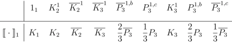
Example 1.3.4. In the Theory of Graphs, our notation makes computing the downward operator easy when the smaller type is0. See Tables 1.4, 1.5 and1.6for some examples in this theory.
11 K21 K2 1
K3 1
P3 1,b
P31,c K31 P31,b P3 1,c
J·K1 K1 K2 K2 K3 2 3P3
1
3P3 K3 2 3P3
1 3P3
Table 1.4: Downward operator in the Theory of graphs from type 1 to type 0 (the function η
is omitted from the notation).
Homomorphism extensions 17
1E P3
E
P3E,c K3E P3E,b
J·KE,η1 K 1 2
1 2P3
1,b
P31,c K31 1 2P
1,b
3
J·KE,η2 K 1 2
1 2P3
1,b 1
2P 1,b
3 K31 P 1,c
3
J·KE K2 1 3P3
1
3P3 K3 1 3P3
Table 1.5: Downward operator in the Theory of graphs from type E to types 1 and 0. The function ηi: [1]→[2] is such that η(1) = iand the function η is omitted from the notation
for type 0.
1E K3
E
P3
E,b
P3
E,c
P3E
J·KE,η1 K2 1
K3 1 2P3
1,b
P3
1,c 1
2P 1,b
3
J·KE,η2 K2 1
K3 P3
1,c 1
2P3 1,b 1
2P 1,b
3
J·KE K2 K3 1 3P3
1 3P3
1 3P3
Table 1.6: Downward operator in the Theory of graphs from type E to types 1 and 0. The function ηi: [1]→[2] is such that η(1) = iand the function η is omitted from the notation
for type 0.
extension ofσ1, with |σi|=ki fori= 1,2, and if F ∈ Fℓσ2 is a σ2-flag of size ℓ, then
qσ2,η(F) = 1 (ℓ)k2−k1
= 1
ℓ(ℓ−1)· · ·(ℓ−k2+k1+ 1)
.
The next step is to define the finite world analogous of the homomorphism extension, which will be useful in obtaining the extension itself.
Before doing so, recall that if F ∈ Fσ is a σ-flag, we can think of the functional p(·;F)
as an element of the compact metric space [0,1]Fσ
. On the other hand, we can also think of a homomorphismφ ∈Hom+(Aσ,R) as an element w of [0,1]Fσ
, where the coordinate F′ of w is φ(F′), for everyF′ ∈ Fσ.
Definition 1.3.6 ([Raz07, Definition 9]).Let (σ2, η) be a type extension of σ1 and F = (M, θ) ∈ Fσ1-flag such that p((σ
2, η);F) > 0. We define the probability measure PσF2,η
extending F to σ2 through η through the following random experiment. Pick uniformly at random a model embeddingα: [|σ2|]→V(M)ofσ2 in M subject to the restriction thatαis consistent with θ on im(η), that is, subject toα◦η=θ◦η, and definePσ2,η
F as the (discrete)
Borel probability measure over [0,1]Fσ2
of the functional p(·; (M,α)).
18 Flag algebras
Definition 1.3.7. LetXbe a topological space and(Pn)n∈Nbe a sequence of Borel probability
measures onX.
We say that (Pn)n∈N weakly converges to a Borel probability measure P on X if
lim
n→∞
Z
X
f(x)dPn(x) =
Z
X
f(x)dP(x),
for every continuous bounded function f: X→R.
Remark 1.3.8. In the case when X is a metric space, the definition of weak convergence coincides with the definition of convergence in distribution.
We recall now one of the most useful equivalences concerning weak convergence.
Lemma 1.3.9 (Portmanteau).If X is a topological space, (Pn)n∈N is a sequence of Borel
probability measures onX, and Pis a Borel probability measure on X, then the following are equivalent.
• The sequence (Pn)n∈N weakly converges to P;
• For every Borel set A ∈ B(X) of X with P(δ(A)) = 0 (where δ(A) is the boundary of A), we have
lim
n→∞
Pn(A) = P(A);
• For every open setU ⊂X, we have
lim inf
n→∞
Pn(U)>P(U);
• For every closed set C ⊂X, we have
lim sup
n→∞
Pn(C)6P(C).
We present (finally) the homomorphism extensions in the theorem below.
Theorem 1.3.10 ([Raz07, Theorems 3.5 and 3.12]). Let(σ2, η)be a type extension of a non-degenerate type σ1 and let φ∈Hom+(Aσ1,R) be a homomorphism such that φ((σ2, η))>0. Under these circumstances, there exists a random element φσ2,η of Hom+(Aσ2,R), called
homomorphism extension of φ to type σ2 through η, satisfying
E[φσ2,η(f)] = φ(JfKσ2,η)
φ(J1σ2Kσ2,η)
, (1.2)
for every f ∈ Aσ2.
Furthermore, the distribution of φσ2,η is unique, that is, if Pσ2,η is the probability measure ofφσ2,η
, and P′ is another probability measure on the Borel sets of Hom+(Aσ2,R) satisfying (1.2), thenPσ2,η =P′.
Moreover, if (Fn)n∈N is a sequence ofσ1-flags converging toφ, then the sequence of
proba-bility measures(Pσ2,η
Fn )n∈Nweakly converges to the probability measure of the extensionφ
σ2,η
(as a random element of [0,1]Fσ2 ).
Interpretation homomorphisms 19
1.4
Interpretation homomorphisms
In this section, we will present the interpretation homomorphisms, which are algebra homomorphisms between flag algebras of different types (and even in different theories) that will codify classical combinatorial arguments of many sorts. We choose to first present the definitions and properties of the interpretation homomorphisms leaving the intuition and examples to the end of the section2.
We start with the definition of flag interpretation, which corresponds to a model interpre-tation followed by the removal of constants that have are not translations of other constants (see Appendix A for the concepts of open interpretation and model interpretation).
Definition 1.4.1.Let T1 andT2 be two universal theories in languages with equality, but no constant or function symbols. Letσ1andσ2 be non-degenerate types inT1 andT2 respectively, and of sizes k1 and k2 respectively.
Recall the definitions of Tσi
i and of Fσi[Ti] and suppose (U, I) : T1σ1 T2σ2 is an open interpretation, let c1, c2, . . . , ck1 be the constant symbols of T
σ1
1 and c′1, c′2, . . . , c′k2 be the constant symbols of Tσ2
2 and define the functionη: [k1]→[k2]to be such that I(ci) =c′η(i) for every i∈[k1].
Note that I applied to the formula Vk1
i,j=1(i=j ⇐⇒ci =cj)implies that η is injective.
Let Fσ2,U[T2] denote the set of allσ
2-flags that areU-models of T2σ2 and for every ℓ∈N, let Fσ2,U
ℓ [T2] =Fσ2,U[T2]∩ F σ2
ℓ [T2].
Suppose F = (M, θ)∈ Fσ2,U[T
2] is a U-model. Then the model interpretation of F is a flag I(F) = (N, θ◦η) of T1 with V(N) =V(M).
We define then the flag interpretation of F as the σ1-flag
I′(F) = I(F)−θ([k2]\η([k1])) =I(F)|V(I(F))\θ([k2]\η([k1])).
Remark 1.4.2. The only case when a flag interpretation coincides with the model interpre-tation is when both types are of the same size.
Theorem 1.4.3 ([Raz07, Theorem 2.6]).With the same definitions and notation of Defini-tion 1.4.1, let
u= X
F∈Fσ2,U k2+1[T2]
F
be the sum of all U-models of size k2 + 1 (that is, the U-models that have exactly one unlabelled vertex) and suppose that u is not a zero divisor in Aσ2[T2].
LetAσ2
u [T2]denote the localization of the algebraAσ2[T1]with respect to the multiplicative system {uℓ : ℓ ∈ N} (that is, every element of Aσ2
u [T2] is of the form u−ℓf for ℓ ∈ N and f ∈ Aσ2[T2]).
For every σ1-flag F1 ∈ Fℓσ11[T1]of size ℓ1, define
π(U,I)(F1) = 1
uℓ1−k1
X
F2∈Fσ2,U[T2]:
I′(F2)∼=F
1
F2 ∈ Aσu2[T2],
and extend the operator π(U,I) linearly to RFσ1[T
1] (note that I′(F2) ∼= F1 implies |F2| =
ℓ1−k1+k2).
2
![Table 1.5: Downward operator in the Theory of graphs from type E to types 1 and 0. The function η i : [1] → [2] is such that η(1) = i and the function η is omitted from the notation for type 0](https://thumb-eu.123doks.com/thumbv2/123dok_br/18477313.366513/39.892.268.603.107.282/table-downward-operator-theory-function-function-omitted-notation.webp)