Effects of Measurement Errors on Population Estimates from Samples Generated from a Stratified Population through Systematic Sampling Technique

(1)

EJ

E c o n o m i c s . E x p e r t J o u r n a l s . c o m

Effects of Measurement Errors on Population Estimates from Samples

Generated from a Stratified Population through

Systematic Sampling Technique

Abel OUKO

1*

_,

_{Cheruiyot W. KIPKOECH}

2

_,

_{Emily KIRIMI}

3

1_{The East African University, Kenya} 2_{Maasai Mara University, Kenya}

3_{Technical University of Kenya}

In various surveys, presence of measurement errors has led to misleading results in estimation of various population parameters. This study indicates the effects of measurement errors on estimates of population total and population variance when samples are drawn using systematic sampling technique from a stratified population. A finite population was generated through simulation. The population was then stratified into four strata followed by generation of ten samples in each of them using systematic sampling technique. In each stratum a sample was picked at random. The findings of this work indicated that systematic errors affected the accuracy of the estimates by overestimating both the population total and the population variance. Random errors only added variability to the data but their effect on the estimates of the population total and population variance was not that profound.

Keywords: Measurement errors, Systematic Errors, Stratified population, Population Total and Population Variance

JEL Classification: P42, R23

1. Introduction

The ultimate goal of each survey is to obtain information about the population under study. The theory of sample survey as developed during the past several decades provides us with various kinds of scientific tools for drawing samples and making valid inference about the population parameters of interest. According to Koninj (1973), in measurement of physical quantities the personnel and devices that we have to use may not give as precise measurements as the best available. Measurement errors cannot be completely eliminated but minimized to an extent which their effects on survey results are not that profound. Basic contributions to the methodology of measurement error models were given by Mahalanobis (1946), Hansen (1946) and Sukhatme and Seth (1952) have examined the question of non sampling errors in census and survey work and they have furnished mathematical models for such errors. The objective of this study was to investigate the effects of measurement errors on the estimates of population total and population variance when samples are drawn from a stratified population using systematic sampling technique. The contribution of this study is to establish more weight as to why systematic errors should be minimized if at all valid results are to be obtained.

*_{Corresponding Author:}

Abel Ouko, Department of Mathematics, The East African University, Kenya Article History:

Received 24 October 2014 | Accepted 4 November 2014 | Available Online 25 November 2014

Cite Reference:

(2)

2. Systematic sampling

This is a sample selection technique in which sample members are selected from a given population according to a random starting point and a fixed periodic interval. Systematic sampling is still thought of as being random, as long as the periodic interval is determined beforehand and the starting point is random. A common way of selecting members into the sample using systematic sampling is simply by dividing the total number of units in the population by the desired number of units for the sample. The result of the division serves as the marker for selecting sample units from within the given population. Systematic sampling is to be applied only when the given population is logically homogeneous because systematic sample units are uniformly distributed over the population. In some cases systematic sampling is preferred since it spreads the sample more evenly over the population and easier to conduct.

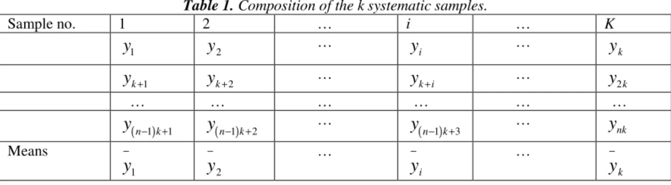
Table 1. Composition of the k systematic samples.

Sample no. 1 2 … i … K

1

y y2 … yi … yk

1

k

y ₊ y_k₊₂ … y_{k i}₊ … y₂_k

… … … … … …

( )n 1k 1

y

₋ ₊

y

_{( )}_n₋₁_k₊₂ …

( )n 1k 3

y

₋ ₊ … ynk

Means

1

y

−

2

y

− …

i

y

− …

y

−_k

2.1.Stratified Systematic sampling.

This is whereby the finite population under study is divided into relatively homogeneous groups referred to as strata and then systematic sampling is carried out in each stratum to generate samples.

Notations: h

N - Total number of units in stratum h where {h =1, 2, ..., H}

h

n - Number of units in a sample drawn from stratum h

hk

µ

- The true value of the

k

th unit in stratum h.

hk

y - is the observed value of the

k

th in stratum h. Note that N =N₁+N₂+...+N_H

3. Sampling design

In the theory of finite population sampling, a sampling design specifies for every possible sample its probability of being drawn. It is convenient to have special notation for this probability which in this case will be P(s).

In other words we assume there is a function P (.) such that P(s) gives the probability of selecting specified samples under the scheme in use. The function P (.) will be referred to as sampling design.

4. The Simple Measurement Model

In this case we would like to formulate a statistical model for measurements made on elements of a sample from a finite population. Consider a finite population, U = {1…, k,…, N}.It is assumed that for each element

k U

∈

, there exists a true value

µ

_k and that the objective is to estimate the population total of these true values,

k U

(3)

A sample s of size n_s is selected from U by a given probability sampling design

p

( )

.

. The idea is to obtain the true value

µ

_k for each element

k

∈

s

, but what we actually obtain through the measurement procedure are the observed values y_k for

k

∈

s

.The observed y_k is composed of the true value

µ

_k and a random error or both random error and systematic error y_k −

µ

_k. For lack of better values, y_k is used in the estimation. For a given sample s, the random variables

y

k

(

k

∈

s

)

are assumed to have a certain joint

probability distribution (conditional on s), called a measurement model denoted by m. In this case we consider our survey as a two stage process whereby the first stage involves the sample selection, which results in a selected sample s and the second stage involves the measurement procedure, which generates an observed value y_k for each

k

∈

s

. When evaluating expectations and variances with respect to the two stages jointly, the conditional argument is useful. As for the expected values,

( )

.

( )

. /

pm p m

E

=

E



_

E

s



_

Where

E

_m

( )

. /

s

denotes conditional expectation with respect to the measurement model m, for a given sample s,

E

_p

( )

.

denotes expectation with respect to the sample design

p

( )

.

and

E

_pm

( )

.

denotes expectation with respect to sampling design and measurement model jointly.

Similarly, for the joint variance, called the pm-variance or the total variance, we have

( )

.

( )

. /

( )

. /

pm p m p m

V

=

E V



_

s



_

+

V



_

E

s



_

Where

V

m

( )

. /

s

denotes conditional variance with respect to the model m, given s,

V

p

( )

.

denotes

variance with respect to

P

( )

.

and

V

_pm

( )

.

denotes variance with respect to

P

( )

.

and m jointly.

We specify further the model m. For element k and l belonging to the same sample s, the first and second moments are

(

/

)

k

E

m

y

k

s

µ

=

(

)

2

/

k

V

m

y

k

s

σ

=

And

σ

_kl

=

C

_m

(

y y

_k

,

_l

/

s

)

5. Measurement errors.

Measurement is the basis of any scientific study. All measurements are, however, approximate values (not true values) within the limitation of measuring device, measuring environment, process of measurement and human error. Several measurements of the same quality on the same subject will not in general be the same.

Measurement errors refer to errors in survey responses arising from the method of data collection, the respondent or the questionnaire. They include the errors in a survey response as a result of respondents confusion, ignorance, carelessness, or dishonesty; the errors attributable to the interviewer, perhaps as a consequence of the poor or inadequate training, prior expectations regarding respondents’ response etc. These measurement errors end up causing a considerable effect on survey estimates. These errors are broadly classified in two categories which are systematic errors and random errors

Systematic errors are biases in measurement which lead to the situation where the mean of many separate measurements differs significantly from the actual value of the measured attribute. All measurements are prone to systematic errors, often of several different types. The errors of this category are characterized by deviation in one direction from the true value. Systematic errors may result from; Usage of faulty instrument, Usage of faulty measuring process and Personal bias. Clearly this type of error cannot be minimized by repeated measurements. Systematic errors can therefore lead to either overestimation or underestimation of the desired population parameters.

(4)

action in exactly the same manner. Hence it is likely that the same person reports different values with the same instrument, which measures quality correctly. This error is caused by any factor that randomly affects the sample. Random errors add variability to the data but do not affect the average performance for the group. This is why at times it is regarded as ‘noise’.

5.1.Mathematical model for measurement errors.

According to Cochran (1977), we assume a large number of independent repetitions of the measurement on the ith unit are possible. Let y_i_α be the value obtained in the

α

th repetition.

Then

y

_i_α

= +

µ

_i

e

_i_α

Where

µ

_i= true value

i

e

_α= measurement error

Where the expectation ofe_ijis zero and variance is

σ

_i2.

[ ]

2

0

i

i i

E e

Var e

α

α σ =

=

Therefore,

[

]

[

]

2

/

i i

E y i

V y i

α

µ

σ

=

6. Inclusion probability in a stratified population

Suppose we have a stratified population containing H number of strata. If we take one stratum denoted by h, our indicator variable becomes,

1

0

( )

th

if the k unit is included in the sample from stratum h

hk

otherwise

I

s

=







Our first order inclusion probability is denoted by

π

_hk which denotes the probability that element k

from stratum h is included into the sample. In the case of systematic sampling, because each element k belongs to one of the 'ah' equally probable systematic samples in stratum ‘h’, (where ah is the sampling interval in

stratum h.)

1

hk h

a

π

=

The second order inclusion probability is denoted by

π

_hkl which refers to the probability that both elements ‘k’ and ‘l’ from stratum h are included into the sample. Under systematic sampling in stratum h

1

0

h

if k and l from stratum h are in same systematic sample

a hkl

otherwise

π





=







(5)

[

( )]

[

( )]

(1

)

hk hk

hk hk hk

E I

s

V I

s

π

=

−

Covariance

cov[

I I

_{hk hl}

]

=

π

_hkl

−

π π

_hk _hl

Since in stratum h our sampling interval is a_h we will have a_h systematic samples in the stratum indicated by s_rwhere r=1, 2,...,ah

7. Horvitz Thompson estimator in a Stratified Population

According to Horvitz and Thompson (1952), the estimator of the population total is given by

1 1

h

n H

hk HT

h k hk

y

t

π

∧

= =

=

∑∑

Its variance is given by,

(

)

(

)

2

1 1 1 1

1

h h h

N N N

H H

hk hk hl

HT hk hkl hk hl

h k hk h k k l hk hl

y

y y

V t

π

π π

π

π π

∧

= = = = ≠





₌

₋

₊

₋









∑∑

∑∑∑

According to Sarndal(1992) there is no unbiased estimator of the variance of estimated population total when a sample is generated using systematic sampling technique. A precise estimator below was then chosen

1

2 2

1

2

1

1 1

r

r r r

H

HT h hHT h

H

h HT _h _hs

h h

hs _hs hk hs h

V t V t

f

V t N S

n

where S y y

n

∧ ∧ ∧ ∧

= ∧ ∧

=

−

 ₌  

   

   

−

 

=

 

 

 

=  − 

−  

∑

Where h h

h

n f

N

= represents the sampling fraction

8. The Mean Square Error (MSE)

The mean square error (MSE) of an estimator is one of the many ways to quantify the difference between values implied by an estimator and the true values of the quantity being estimated. The difference occurs because of randomness or because the estimator does not account for information that could produce a more accurate estimate. In order to compare a biased estimate with unbiased estimate or two estimates that have different amounts of bias, a useful criterion is the ‘mean square error’ of the estimate measured from the population value that is being estimated. Formally,

(

)

(

)

(

)

(

)

2 2

2

MSE E E m m

E m m E m m

Variance of bias

µ µ µ µ µ

µ µ µ µ

µ

∧ ∧ ∧

∧ ∧

∧

 

     

= − = − + −

  _ _ _  _

      

   

=  −  + −  − + −

   

 

= +

(6)

The cross product term varnishes since_E__µ∧₋_m_ ₌₀

  . The use of the MSE as a criterion of the

accuracy of an estimate amounts to regarding two estimates that have the same MSE as equivalent. This is not strictly correct because the frequency distribution of errors __{µ µ}∧₋ _

  of different sizes will not be the same for

the two estimates if they have different amounts of bias.

9. Total variance of the estimator of the population total in absence of systematic errors

The total variance in the absence of systematic errors is obtained as follows. Since our population is stratified our measurement model is y_hk =

µ

_hk+e_hk

Where

(

)

(

)

(

)

2

/

,

m hk hk m hk hk

m hk hl hkl

E

y

s

k

s

V

y

s

k

s

Cov

y y

s

k l

s

µ

σ

=

∈

=

∈

=

∈

The total variance is given by

/

HT HT HT

pm p m p m

V

t

V E

t

s

E V

t

s

∧

_

∧

_

_

∧

_













=

+





_





_

_





_





















Where 1 1 1 1 2 2

1 1 1 , 1

2

1 1 1 , 1

h

a

h h h h

r a

h h h h

r

n H

hk HT

p m p m

h k hk

s

n n n

H H

hk hkl

p

h k hk h k l s k k l hk hl

s

N N N

H H

hk hkl hkl

y

E V

t

E V

E

π

σ

π

π π

σ

σ π

π

π π

= = ∧ = = = = = ∈ = ≠ = = = ∈ = ≠

















=















_

_







_

_

_

_





=



_

+



_





=

+

∑∑

∑ ∑ ∑∑

∑∑

∑ ∑ ∑∑

(

)

(

)

1 1 1 1 1 2

1 1 1 , 1

1

h

a

h h h h

r

n H

hk HT

p m p m

h k hk

n H

hk p

h k hk

s

N N N

H H

hkl hk hl hk

hk hk hl

y

V E

t

V E

V

π

µ

π

π π

µ

_π

_{µ µ}

π

₌

π π

∧ = = = = = = = ∈ = ≠

















=















_

_



















=









−

=

−

+

∑∑

∑ ∑ ∑∑

Therefore the total variance in absence of systematic errors is given by

(

)

(

)

1 1

2 2

1 1 1 , 1 1 1 1 , 1

1

a a

h h h h h h h h

r r

s s

N N N N N N

H H H H

hkl hk hl

hk hkl hkl hk

HT

pm hk hk hl

h k hk h k l s k k l hk hl h k hk h k l s k k l hk hl

V

t

σ

σ π

µ

π

π π π

µ µ

π

=

π π

π

=

π π

(7)

By replacing both first and second order inclusion probabilities with 1

h

a the variance becomes

( )

1 1

2 2

1 1 1 , 1 1 1 1 , 1

1

a a

h h h h h h h h

r r

s s

N N N N N N

H H H H

HT

pm h hk h hkl h hk h hk hl

h k h k l s h k l h k h k l s k k l

V

t

a

σ

a

σ

a

µ

a

µ µ

= =

∧

= = = ∈ = ≠ = = = ∈ = ≠





=

+

−

+

−









∑∑

∑∑∑∑

∑∑

∑∑∑∑

10. The mathematical model for measurement of errors in stratified population

Since our population is stratified, the model becomes

hk hk hk

y =

µ

+e

hk

µ

- represents the true value of unit k in stratum h

hk

e - represents the measurement error term of unit k in stratum h

(

/

)

m hk hk hk

E

y

s

b

µ

k

s

∴

=

+

∈

Where b_hk refers to the bias term

(

)

2

/

m hk hk

V

y

s

=

σ

k

∈

s

The covariance between

k

th and

l

th unit is

(

/ ,

)

( )

m hk hl hk hk hk hk

Cov

y y

k l

∈ =

s

E y



_

−

E Y

 

_{ }

y

−

E y



_

(

)(

)

(

)

(

/ ,

)

hk hk hl hl hk hl

m hk hl hkl

E e

b

e

b

Cov e e

Cov

y y

k l

s

σ

=

−

=

∴

∈ =

11. Decomposition of the mean square error.

In this case we will consider the Horvitz Thompson estimator and the effect of measurement errors on its accuracy. We will decompose the mean square error into components, assuming that the measurements

obey the simple measurement model ‘m’ as stated before. The mean square error of

t

HT ∧

can be written as the sum of the total variance and squared bias.

2

HT HT HT

pm pm pm

MSE

t

V

t

B

t

∧ ∧

_

∧

_













=

+









_





_

















The total variance is given by

2

HT HT HT

pm pm pm

V

_



t

∧

_



=

E

_



t

∧

−

E

_



∧

t



_



_













The bias is given by

B

pm

t

HT

E

pm

t

HT

t

µ

∧ ∧









=

−

















This is called the measurement bias, which arises when expected measurement values on elements do not agree with true values. Variance term can be decomposed as follows

1 2

/

HT HT HT

pm p m p m

V

_



∧

t

_



=

V



_

E

_



t

∧

s



_

_



+

E V



_



_

∧

t

s

_





_

= +

V

(8)

The first component

V

₁ is referred to as the sampling variance which is zero in the case of complete enumeration whereas the second component

V

₂ is referred to as the measurement variance. The Horvitz Thompson estimator for the population total in this case will be

1 1 h n H hk HT

h k hk

y

t

π

∧ = =

=

∑∑

But,

[ ]

1 1 1 1 1 1 1 1

1 1 1 1

sin

h h h h h h n H hk HT

pm p m

h k hk

n H

hk

p hk hk hk

h k hk

N H

hk

p hk

h k hk

N H

hk p hk hk

h k

N N

H H

hk hk

h k h k

y

E

t

E

g

E

where

g

b

g

E

I

g

ce

E

I

b

π

µ

π

µ

∧ = = = = = = = = = = = =













=

















_

_

_

_





=





=

+





=

+

∑ ∑

From the decomposition of the variance term, we have

V

₁

&

V

₂where

[ ]

(

)

1 1 2 1 1 1 1 1 2 2

1 1 , 1

c o v

h h a

h h h h

r

H T H T

p m p m

n H

h k H T

p m p m

h k h k n

H

h k p

h k h k s

N N N

H

h k h k h l

h k h k k l s k k l h k h l

V

E

t

V

E

V

t

y

V

E

t

V

E

g

V

g

V

I

π

₌

π

∧ ∧ ∧ = = = = = = ∈ = ≠

















=

_





_

=

_





_

































∴

=

_





_

=

















_

_

_

_





=









=

+

∑ ∑

∑ ∑ ∑

1 H h=

∑

[ ]

(

)

(

) (

)

(

)

(

)

(

)

(

)

1 1 2 1 2

1 1 1 , 1

2

1 1 1 , 1

1 cov

1

a

h h h h

r a

h h h h

r

hk hk hk hk hl hkl hk hl

s

N N N

H H

hk hk hl

hk hk hkl hk hl

s

N N N

H H

hkl hk hl hk

hk hk h

But

V I

and

I I

g

V

g

g g

π

π π

π

π π

π

π π

π

π π

π

π π

= = = = = ∈ = ≠ = = = ∈ = ≠

=

−

=

−

∴ =

−

+

−

=

−

+

∑∑

∑ ∑ ∑∑

∑∑

∑ ∑ ∑∑

l

hk hk hk hl hl hl

(9)

(

₎₍

₎

(

₎₍

₎

(

)

₍

₎

(

)

1 1 2 1

1 1 1 , 1

2 2

1 1 1 , 1

1

2

a

h h h h

r

a

h h h h

r s

N N N

H H

hk hkl hk hl

hk hk hk hk hl hl h k hk h k l s k k l hk hl

s

N N N

H H

hk hkl hk hl

hk hk hk hk hk hl hk hl hl hk hk h k hk h k l s k k l hk hl

V

b

b b

π

π π

µ

π

π π

π

π π

µ

µ µ µ

µ

π

π π

= = = = = ∈ = ≠ = = = ∈ = ≠

−

=

+

−

=

+

∑∑

∑ ∑ ∑∑

∑∑

∑ ∑ ∑∑

(

hl

)

(

)

(

)

(

)

(

)

(

)

(

)

1 1 2 1

1 1 1 , 1

2

1 1 1 , 1

1 1

1

2

a

h h h h

r a

h h h h

r h

s

N N N

H H

h k h k l h k h l

h k h k h l

h k h k h k l s k k l h k h l s

N N N

H H

h k h k l h k h l

h k h k h l

h k h k h k l s k k l h k h l N

H

h k h k l h k h l h k h l

h k h k h k h

V

b

b b

b

π

_µ

π

π π

_{µ µ}

π

π π

π

π π

π

π π

π

_µ

π

π π

π

π π

= = = = = ∈ = ≠ = = = ∈ = ≠ = =

−

=

+

−

+

−

+

∑ ∑

∑ ∑ ∑ ∑

∑ ∑

∑ ∑ ∑ ∑

∑ ∑

1

1 , 1

a h h h

r

s N N H

h k h l h k l s k k l l

b

µ

= = ∈ = ≠















∑ ∑ ∑ ∑



1 2 1 1 2

1 1 1 , 1

h

a

h h h h

r H T p m n H h k p m

h k h k

s

N N N

H H

h k h k l h k l

h k h k h k l s k k l h k h l

V

E

V

t

y

E

V

π

σ

σ π

π

₌

π π

∧ = = = = = ∈ = ≠









=

_





_

















=

















=

+

∑ ∑

∑ ∑ ∑ ∑

Thus the total variance in presence of measurement errors is

/

HT HT HT pm p m p m

V





∧

t





=

V



_

E





∧

t

s







_

+

E



_

V





t

∧

s







_





















=

V

₁

+

V

₂

(

)

1

2

1 1 1 , 1 1

2

1 1 1 , 1

1

a

h h h h

r a

h h h h

hl

r hk

s

N N N

H H

hk hkl hkl

h k hk h k l s k k hk hl

s

N N N

H H

hkl hk hk

hk hk hl

h k h k l s k k l hk hl

σ

σ π

π

π π

π π π

π

µ

µ µ

π

π π

(10)

(

)

(

)

1

2

1 1 1 , 1

1

2

a

h h h h

r

a

h h h h

r s

N N N

H H

hk hkl hk hl

hk hk hl

s

N N N

H H

hk hkl hk hl

hk hk hk hl

b

b b

b

π

π π

π

π π

π

_µ

π

π π

_µ

π

π π

=

= = = ∈ = ≠

−

+



₋



+



_

+



_





∑∑

∑ ∑ ∑∑

∑∑

∑ ∑ ∑∑

Under systematic sampling in populations with stratification as previously obtained the inclusion probabilities are:

1

hk h

a

π

=

1

0

h

if k and l from stratum h are in same systematic sample

a hkl

if k and l from stratum h are in different systematic samples

π





=







We then substitute these probabilities in

/

HT HT HT

pm p m p m

V

t

V

E

t

s

E V

t

s

∧

_

∧

_

_

∧

_













=

+





_





_

_





_





















(

)

(

)

1

2

1 1 1 , 1 1

2

1 1 1 , 1

2

1 1 1

1

a

h h h h

r

a

h h h h

hl r

hk

h h h

s

N N N

H H

hk hkl hkl h k hk h k l s k k hk hl

s

N N N

H H

hkl hk hk

hk hk hl

h k h k l s k k l hk hl

N N N

H

hk hkl hk hl

hk hk hl

h k hk k k l hk hl

b

b b

σ

σ π

π

π π

π

π π

π

_µ

_{µ µ}

π

π π

π

π π

π

π π

=

= = = ∈ = ≠

= = = ≠

=

+

−

+

−

+

∑ ∑

∑ ∑ ∑ ∑

∑ ∑

∑ ∑ ∑ ∑

∑ ∑

(

)

1

1 ,

1 1 1 , 1

1

2

ah r

a

h h h h

r s

H h k l s

s

N N N

H H

hk hkl hk hl hk hk hk hl h k hk h k l s k k l hk hl

b

π

_µ

π

π π

_µ

π

π π

= =

= ∈

= = = ∈ = ≠



₋



+



_

+



_





∑ ∑

∑ ∑ ∑ ∑

We then replace both the first and second order inclusion probabilities with 1

h

(11)

1 2

1 1 1 , 1

2

1 1 1

1

1 1 1

1 1

1 1 1

a

h h h h

r

h h h

hkl s

N N N

H H

h hk

pm HT

h k h k l s k k l

h h h

N N N

H

h h h

h hk

h k k k l

h h h

a

V t

a a a

a

a a a

σ

µ

= ∧ = = = ∈ = ≠ = = = ≠      ₌ ₊     _ _ _ _{ } _                       − −                   + +                  

∑∑

∑ ∑ ∑∑

∑∑

1 1 , ah r s H hk hl h k l s

µ µ

= = ∈

∑ ∑

1 1 2

1 1 1 , 1

, 1

1

1 1 1

1

2

1 1 1

a

h h h h

r

ah h h r s

N N N

H H

h h h h

hk hk hl

h h h

s N N

h h h h

hk hk hk hk h k l s k k l

h h h

a

b

b b

a

a a

b

a

a a

µ

= = = = = ∈ = ≠ ∈ = ≠



     







−



     







     









+

 

   

 

   

 

   









−

















+

∑∑

∑ ∑ ∑∑

∑ ∑∑

1 1 1

h N

H H

h= k= =





























∑∑

∑

This then simplifies to

(

)

(

)

(

)

(

)

(

)

1 1 1 2

1 1 1 , 1

2

1 1 1 , 1

2

1 1 1 , 1

1

2

1

a

h h h h

r a

h h h h

r a

h h h h

r

s

N N N

H H

HT

pm h hk h hkl

s

N N N

H H

h hk h hk hl

s

N N N

H H

h hk h hk hl

h hk hk

V

t

a

b

a

b b

a

b

σ

µ

µ µ

µ

= = = ∧ = = = ∈ = ≠ = = = ∈ = ≠ = = = ∈ = ≠





=

+









+

−

+

−

+

−

+

−

+

−

+

∑∑

∑ ∑ ∑∑

∑∑

∑ ∑ ∑∑

∑∑

∑ ∑ ∑∑

(

)

1

1 1 1 , 1

1

a

h h h h

r

s

N N N

H H

h hk hl

a

µ

b

= = = = ∈ = ≠





−











∑∑

∑ ∑ ∑∑



12. Simulation of a finite population

Visual basic programming language along with Microsoft access were used to generate a finite population of size N=1000. A population was simulated containing true values ranging from 20 to 90 inclusive. The true values had a normal distribution with a mean of 55 and a variance of 100. The population was then subdivided into four strata. This was done by first arranging all the population units in ascending order. The first 300 units were selected to constitute the first stratum and the following 250 units were selected to constitute the second stratum. The third and fourth strata were also selected to contain 250 and 200 units respectively. A sampling interval of 10 was used in each stratum resulting to 10 systematic samples in each stratum. In each stratum a sample was selected at random. In this case an assumption was made that systematic error

b

_hkis proportional to the true value

b

_hk

=

d

µ

_hk

(12)

13. Results

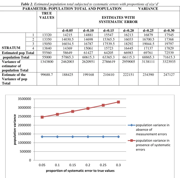
Table 2. Estimated population total subjected to systematic errors with proportions of size‘d’ PARAMETER: POPULATION TOTAL AND POPULATION VARIANCE

TRUE

VALUES ESTIMATES WITH

SYSTEMATIC ERROR

d=0.05 d=0.10 d=0.15 d=0.20 d=0.25 d=0.30

STRATUM

1 13320 14215 14881 15547 16213 16879 17545

2 13350 14030.5 14698 15365.5 16033 16700.5 17368

3 15050 16034.5 16787 17539.5 18292 19044.5 19797

4 13840 14369 15061 15723 16445 17137 17829

Estimated pop Total 55560 58649 61427 64205 66983 69761 72539

population Total 55000 57865.3 60615.3 63365.3 66115.3 68865.3 71615.3 Variance of

estimator of population Total

1343800 2462003 2620951 2786619 2959005 3138111 3323935

Estimate of the Variance of pop Total

99688.7 188425 199168 210410 222151 234390 247127

Figure 1. Effects of systematic errors on variance of estimated population total

14. Conclusion

The table 2 and figure 1 indicated that there was an increase in population total and population variance with increase in systematic error. The findings of the study indicated that systematic errors had a significant impact on the accuracy of the estimates of both population total and population variance.

15. References

Cochran, W.G., 1977. Sampling techniques. 3rd_{Edition, John Willey and Sons, New York.}

Hansen, M. H., and Hurwitz, W. N., 1946. The problem of non-response in sample surveys. Journal of the American Statistical Association, 41, pp.517-529

Horvitz D. G. and Thompson D. J, 1952. A Generalization of sampling without replacement from a finite universe. Journal of the American Statistical Association, 47(260), pp.663-685

0 500000 1000000 1500000 2000000 2500000 3000000 3500000

0.05 0.1 0.15 0.2 0.25 0.3

p

o

p

u

lat

io

n

v

ar

ian

ce

proportion of systematic error to true values

population variance in absence of

(13)

Koninj H.S., 1973. Statistical theory of sample survey design and analysis. North Holland Publishing Company, Amsterdam.

Mahalanobis, P.C., 1946. Recent experiments in statistical sampling in the Indian statistical institute.Journal of the Royal Statistical Society, 325-370.

Sarndal, C.E., Swensson, B., and Wretman, J., 1992. Model assisted survey sampling. New York, Springer Verlag.

Suhkatme, P.V., and Seth, G.R., 1952. Non-sampling errors in surveys. Journal of Indian Society of Agricultural Statistics, 5-41.