Towards space based verification of CO<sub>2</sub> emissions from strong localized sources: fossil fuel power plant emissions as seen by a CarbonSat constellation

(1)

AMTD

4, 5147–5182, 2011

Towards space based verification of CO₂

emissions

V. A. Velazco et al.

Title Page

Abstract Introduction

Conclusions References

Tables Figures

◭ ◮

Back Close

Full Screen / Esc

Printer-friendly Version

Interactive Discussion

Discussion

P

a

per

|

Dis

cussion

P

a

per

|

Discussion

P

a

per

|

Discussio

n

P

a

per

|

Atmos. Meas. Tech. Discuss., 4, 5147–5182, 2011 www.atmos-meas-tech-discuss.net/4/5147/2011/ doi:10.5194/amtd-4-5147-2011

Atmospheric Measurement Techniques Discussions

This discussion paper is/has been under review for the journal Atmospheric Measure-ment Techniques (AMT). Please refer to the corresponding final paper in AMT

if available.

Towards space based verification of CO

₂

emissions from strong localized sources:

fossil fuel power plant emissions as seen

by a CarbonSat constellation

V. A. Velazco, M. Buchwitz, H. Bovensmann , M. Reuter, O. Schneising, J. Heymann , T. Krings , K. Gerilowski, and J. P. Burrows

Institute of Environmental Physics (IUP), University of Bremen, Germany

Received: 13 July 2011 – Accepted: 9 August 2011 – Published: 12 August 2011 Correspondence to: V. A. Velazco ([email protected])

(2)

AMTD

4, 5147–5182, 2011

emissions

Title Page

Tables Figures

◭ ◮

Back Close

Full Screen / Esc

Discussion

P

a

per

|

Dis

cussion

P

a

per

|

Discussion

P

a

per

|

Discussio

n

P

a

per

Abstract

Carbon dioxide (CO₂) is the most important man-made greenhouse gas (GHG) that cause global warming. With electricity generation through fossil-fuel power plants now as the economic sector with the largest source of CO₂, power plant emissions mon-itoring has become more important than ever in the fight against global warming. In 5

a previous study done by Bovensmann et al. (2010), random and systematic errors of power plant CO₂emissions have been quantified using a single overpass from a pro-posed CarbonSat instrument. In this study, we quantify errors of power plant annual emission estimates from a hypothetical CarbonSat and constellations of several Car-bonSats while taking into account that power plant CO₂emissions are time-dependent. 10

Our focus is on estimating systematic errors arising from the sparse temporal sampling as well as random errors that are primarily dependent on wind speeds. We used hourly emissions data from the US Environmental Protection Agency (EPA) combined with assimilated and re-analyzed meteorological fields from the National Centers of Envi-ronmental Prediction (NCEP). CarbonSat orbits were simulated as a sun-synchronous 15

low-earth orbiting satellite (LEO) with an 828-km orbit height, local time ascending node (LTAN) of 13:30 (01:30 p.m.) and achieves global coverage after 5 days. We show, that despite the variability of the power plant emissions and the limited satellite overpasses, one CarbonSat can verify reported US annual CO₂emissions from large power plants (≥5 Mt CO₂yr−1) with a systematic error of less than ∼4.9 % for 50 % of all the power 20

plants. For 90 % of all the power plants, the systematic error was less than∼12.4 %. We additionally investigated two diﬀ_{erent satellite configurations using a combination}

of 5 CarbonSats. One achieves global coverage everyday but only samples the targets at fixed local times. The other configuration samples the targets five times at two-hour intervals approximately every 6th day but only achieves global coverage after 5 days. 25

(3)

AMTD

4, 5147–5182, 2011

emissions

Title Page

Tables Figures

◭ ◮

Back Close

Full Screen / Esc

Discussion

P

a

per

|

Dis

cussion

P

a

per

|

Discussion

P

a

per

|

Discussio

n

P

a

per

|

somewhat smaller for the CarbonSat constellation configuration achieving global cov-erage everyday. Finally, we recommend the CarbonSat constellation configuration that achieves daily global coverage.

1 Introduction

Carbon dioxide (CO₂), a major greenhouse gas that contributes to global warming 5

had been at values between 270 and 290 ppm for the past thousand years before industrialization (Forster et al., 2007, FAQ 2.1 Fig. 1). Since the industrial revolution (around 1750 AD), CO₂has increased by 36 % (Forster et al., 2007). Global warming is now recognized as an impending threat to mankind and the ecosystem, driven mainly by the increase of man-made greenhouse gases (GHG). In order to curb the increase 10

of greenhouse gases, legally binding agreements to cut greenhouse gas emissions have been established under the Kyoto protocol. However, compliance, monitoring and verification of emissions is and will still remain a challenge.

Up to three quarters of the atmosperic CO₂ increase have been attributed to fossil fuel combustion (e.g. in power plants, steel plants), gas flaring (at refineries, oil plat-15

forms, etc.) and cement production (Forster et al., 2007). However, despite their impor-tance, these CO₂sources have not been well quantified. For example, the uncertainty in world’s annual fossil fuel emissions is±6 to±10 % (or 0.6 to 1.0 PgC yr−1) (Marland and Rotty, 1984, Marland, 2008). This uncertainty is 1.5 to 3.3 times larger than the uncertainty in the atmospheric CO₂ accumulation (±0.3 to ±0.4 PgC yr−1) (Marland, 20

2008). The uncertainty in fossil fuel emissions is also an important limitation in inver-sion calculations of global carbon mass balance because, as pointed out by Oda and Maksyutov (2011), most common inversion frameworks assume fossil fuel emissions as well known quantities, only biospheric and oceanic fluxes are corrected via opti-mization (e.g. Gurney et al., 2002). As a result, even small uncertainties in the budget 25

(4)

AMTD

4, 5147–5182, 2011

emissions

Title Page

Tables Figures

◭ ◮

Back Close

Full Screen / Esc

Discussion

P

a

per

|

Dis

cussion

P

a

per

|

Discussion

P

a

per

|

Discussio

n

P

a

per

from continental scales to regional, national or urban carbon budgets. As an example to highlight this, Gurney et al. (2005) did a sensitivity study of atmospheric inversions. They illustrated that the lack of seasonality on fossil fuel emissions produced biases of up to 50 % of the seasonal flux estimates during certain times of the year in the US. In another study, Corbin et al. (2010) used a high resolution fossil fuel inventory for the US 5

and showed that regional near-surface CO₂ concentrations are altered by more than 15 ppm when seasonal variablility of fossil fuel emissions was included in their model.

Power plants play a big role in the magnitude of fossil fuel emissions. For instance, in 2009, fossil-fuel power plants supplied about 69 % of the US electricity demand and is responsible for 41 % of the total anthropogenic CO₂emissions in the US (US EPA: 10

www.epa.gov/climatechange/emissions/co2 human.html), making it the economic sec-tor with the largest source of CO₂ (Petron et al., 2008). Although the US has strict emissions reporting laws under the 1990 Clean Air Act, the uncertainties in hourly reported power plant CO₂ emissions using Continuous Emission Monitoring Systems (CEMS) are still up to around 14 % (Peischl et al., 2010). In Europe, under the Eu-15

ropean Union Emissions Trading Scheme (EU ETS) (Ellerman and Buchner, 2007), large CO₂emitters (>500 ktCO₂yr−1, accounting for∼40 % of EU CO₂emissions) are required to report annual emissions and are entitled to emission allowances. Since 1 January 2005, CO₂emission allowances can be bought or sold by more than 11 500 installations accross Europe (Ellerman and Buchner, 2007). The value of the al-20

lowances distributed under the EU ETS (2005–2007) is about $41 billion (at about

€_15/tCO

2, with €1.00=$1.25) (Ellerman and Buchner, 2007). The amount of money

involved makes accurate CO₂reporting valuable. However, Evans et al. (2009) exam-ined the CO₂ calculation approach implemented in the EU ETS and mentioned that it contains a bias that can be up to 20 % against direct measurement. Power plant emis-25

(5)

AMTD

4, 5147–5182, 2011

emissions

Title Page

Tables Figures

◭ ◮

Back Close

Full Screen / Esc

Discussion

P

a

per

|

Dis

cussion

P

a

per

|

Discussion

P

a

per

|

Discussio

n

P

a

per

|

infringe upon sovereignty of countries are required, such as satellites.

SCIAMACHY on ENVISAT (Burrows et al., 1995; Bovensmann et al., 1999) is the first satellite to perform Planetary Boundary Layer (PBL)-sensitive measurements of column-averaged CO₂ and CH₄ mixing ratios (i.e.XCO₂ andXCH₄) using the short-wave infrared and near infrared spectra (Buchwitz et al., 2007, Frankenberg et al., 5

2011, Schneising et al., 2011). There are also a number of satellite instruments that measure tropospheric CO₂ in nadir mode such as HIRS/TOVS (Ch ´edin et al., 2002, 2003), AIRS (Engelen et al., 2004, Engelen and Stephens, 2004, Engelen and Mc-Nally, 2005), IASI (Crevoisier et al., 2009), and TES (Kulawik et al., 2010). These in-struments measure in the thermal infrared (TIR) part of the electromagnetic spectrum, 10

yielding high sensitivity in the middle and upper troposphere but have low sensitiv-ity in the lower atmospheric layers, where the regional GHG source and sink signals are largest. This low sensitivity limits the information content with respect to regional CO₂ and CH₄ sources and sinks. And so, dedicated greenhouse gas satellite instru-ments have been built recently as a response to the urgency of quantifying CO₂ from 15

space; the Orbiting Carbon Observatory (OCO) from the USA’s side (Kuang et al., 2002; Crisp et al., 2004; Miller et al., 2007) and Japan’s Greenhouse Gases Observing Satellite (GOSAT) (Hamazaki et al., 2004; Kuze et al., 2009). These instruments were designed to perform highly accurate and precise global CO₂ (and CH₄ for GOSAT) measurements from space down to the PBL. GOSAT was successfully launched in 20

2009, unfortunately, OCO failed to reach orbit and was lost shortly after its launch on 24 February 2009 (Palmer and Rayner, 2009). However, because of the importance of remote verification of CO₂ emissions from space, the US government under the Obama administration has decided to build OCO-2 (Boesch et al., 2011), an exact copy of OCO, expected to be launch-ready by 2013. Active remote sensing of CO₂ using 25

(6)

AMTD

4, 5147–5182, 2011

emissions

Title Page

Tables Figures

◭ ◮

Back Close

Full Screen / Esc

Discussion

P

a

per

|

Dis

cussion

P

a

per

|

Discussion

P

a

per

|

Discussio

n

P

a

per

possible now and in the near future. To achieve this, and to continue the time series of PBL-sensitive CO₂ and CH₄ observations from space, which started with SCIA-MACHY on Envisat, CarbonSat (Bovensmann et al., 2010) was proposed. And just recently, the potential of remote sensing to determine power plant emission was suc-cessfully demonstrated using an airborne instrument applying the same methodology 5

as proposed for CarbonSat (Krings et al., 2011).

CarbonSat has been selected by the European Space Agency (ESA) to be one of two candidates for the 8th Earth Explorer Opportunity Mission (EE-8) to be launched in 2018 earliest. CarbonSat’s goal is to globally measure atmospheric CO₂ and CH₄ with the precision, accuracy, spatial resolution and coverage needed to provide crucial 10

information on the sources and sinks of these greenhouse gases. Due to the wide coverage (500 km swath width) and high spatial resolution (2 km×2 km) of CarbonSat, its measurements can be used for several applications. One of them is monitoring of greenhouse gas “hot spot” emission sources, such as power plants.

In this paper, we extend the work done by Bovensmann et al. (2010) by utilizing ac-15

tual power plant emissions in the USA combined with high-resolution re-analyzed data of local meteorological conditions (winds and cloud cover). We present a characteri-zation of systematic and random errors that would arise from power plant monitoring using hypothetical CarbonSat constellations. For the systematic errors, we focus on er-rors of annual emission estimates arising from sparse temporal coverage. The random 20

error is due to instrument (detector) noise. The orbits and sampling characteristics were simulated for this purpose. We are able to quantify this type of systematic error because the power plant emissions are known in this study. In reality only the random error is known and the sampling error component has to be estimated e.g. from the results of the study at hand.

25

(7)

AMTD

4, 5147–5182, 2011

emissions

Title Page

Tables Figures

◭ ◮

Back Close

Full Screen / Esc

Discussion

P

a

per

|

Dis

cussion

P

a

per

|

Discussion

P

a

per

|

Discussio

n

P

a

per

|

show the results from the statistical analyses and provide discussions explaining the errors and the diﬀ_{erences between the selected constellation configurations. We also}

attempt to investigate the year-to-year variablity in emissions of some power plants. Conclusions for this study and arguments for a preferred constellation are presented in Sect. 4.

5

2 Data and methods

This section describes the data we used for the statistical analyses, most of which are originally available online from United States government agencies. For this work we focus on power plants in the conterminous United States due to the exemplary strictness of the reporting requirements imposed on electric generation utility power 10

plants in this country.

2.1 Environmental Protection Agency Clean Air Markets-Data and Maps (EPA

CAMD) Emissions Database

Electric Generation Utility (EGU) power plants in the US are required by law to re-port hourly averaged emissions of nitrogen oxides (NO_x), sulfur dioxide (SO₂) and 15

carbon dioxide (CO₂) as indicated under Title 42 of the US code section 7561 k (Peischl et al., 2010). The latest emission data from major power plants are deliv-ered by Continuous Emission Monitoring Systems (CEMS), which determine mixing ratios of NO_x, SO₂ and CO₂ from the stack exhaust of each plant. Hourly emis-sion fluxes are calculated by combining the information on the mixing ratios with 20

stack flow rate measurements. These data are subject to quality control proce-dures and reported to the US Environmental Protection Agency (EPA) every quar-ter. The data are then posted and made available for download at the EPA web-site (http://camddataandmaps.epa.gov/gdm/index.cfm). Diﬀ_{erent contractors perform}

(8)

AMTD

4, 5147–5182, 2011

emissions

Title Page

Tables Figures

◭ ◮

Back Close

Full Screen / Esc

Discussion

P

a

per

|

Dis

cussion

P

a

per

|

Discussion

P

a

per

|

Discussio

n

P

a

per

the stack gases and flow rates. In order for CEMS to be compliant with the US Code of Federal Regulations (C.F.R.), tests must agree to within±10 % for NO_x, SO₂and CO₂ concentrations (with CEMS showing no low bias compared to the tests) and within ±10 % for stack flow rates, as mentioned in Peischl et al. (2010). Assuming random errors are normally distributed, mass emission rates from EGUs equipped with CEMS 5

should be accurate to better than ±14 % (after summing the concentration and flow uncertainties in quadrature) and enhancement ratios (e.g. NO_x/CO₂) should also be accurate to better than ±14 %, assuming the stack flow rate uncertainties are the same for each trace gas measurement (Peischl et al., 2010). Thus, the EPA CAMD data provide a unique, objective and detailed estimation of the CO₂ emissions from power 10

plants (Petron et al., 2008). Petron et al. (2008) further established the robust nature of the CAMD data set by presenting cases of regional-scale emissions anomalies that are apparent in the data set and explaining these anomalies by known events in regional power generation and distribution.

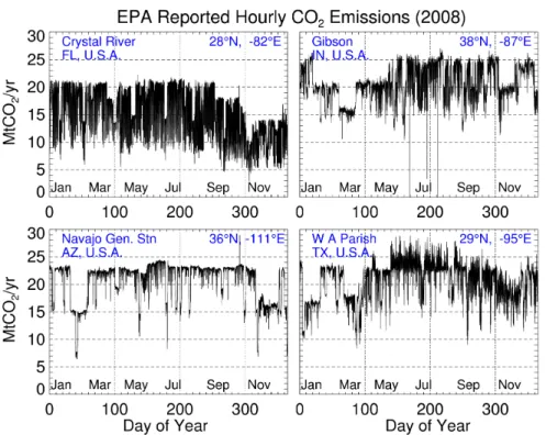
Figure 1 shows the hourly CO₂ emissions from four selected power plants in the 15

US. By making use of the CAMD data, the strong daily, weekly and seasonal cycles of CO₂emissions from power plants can be taken into account in studying the associ-ated errors arising from the sampling characteristics of CarbonSat. For our purpose, we only selected power plants with more than or equal to 1 MtCO₂yr−1_emissions

be-cause (1) CarbonSat error limitations dictate that only power plants emitting above 20

0.8 MtCO₂yr−1

could be measured (Bovensmann et al., 2010) and (2) Power plants emitting more than 1 MtCO₂yr−1 _{are more likely to supply the electricity grid}

continu-ously.

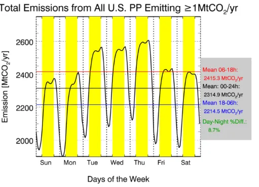
Electrical consumption is not constant throughout the day, so power plants have to adjust their power output according to this demand. This is reflected on the power plant 25

(9)

AMTD

4, 5147–5182, 2011

emissions

Title Page

Tables Figures

◭ ◮

Back Close

Full Screen / Esc

Discussion

P

a

per

|

Dis

cussion

P

a

per

|

Discussion

P

a

per

|

Discussio

n

P

a

per

|

are around 9 % from all power plants. During the day, power demand varies strongly. The peak demand usually happens around mid-morning and around late afternoon. However, since power plants may also supply a city thousands of kilometers away (e.g. Navajo Generating Station supplying Los Angeles∼900 km away), the times of the peak demands may vary. There are also day-to-day variations in the emissions 5

(i.e. weekends have usually lower emissions), making it even more important for an instrument to have short revisit times in order to monitor power plant emissions and capture its variablity from space.

2.2 NCEP-NARR wind vectors and cloud cover

National Centers for Environmental Prediction-North American Regional Reanalysis 10

(NCEP-NARR) is an extension of the NCEP global reanalysis. It is run over the North American region. The NCEP-NARR model uses very high resolution NCEP Eta Model (32 km/45-layer) together with the Regional Data Assimilation System (RDAS). This system assimilates precipitation along with other variables. The improvements in the model/assimilation have resulted in a dataset with substantial improvements in the ac-15

curacy of temperature, winds and precipitation compared to the NCEP-DOE Global Re-analysis 2 (http://www.esrl.noaa.gov/psd/data/gridded/data.narr.monolevel.html). Out-puts of surface (10 m above ground) wind vectors (uandv) and cloud cover are given in 3 h bins, which are then interpolated to the reported hourly emissions of each power plant. NCEP NARR wind and cloud cover data are given in a 32 km×32 km grid. For 20

our purpose, we selected the data points closest to the power plant targets.

2.3 CarbonSat constellation configurations

Studies have been performed on diﬀ_{erent satellite orbit configurations, while taking}

into account the reported CO₂ emissions and the NCEP meteorology. Our first ap-proach was to simulate overpasses from a single CarbonSat satellite with the following 25

(10)

AMTD

4, 5147–5182, 2011

emissions

Title Page

Tables Figures

◭ ◮

Back Close

Full Screen / Esc

Discussion

P

a

per

|

Dis

cussion

P

a

per

|

Discussion

P

a

per

|

Discussio

n

P

a

per

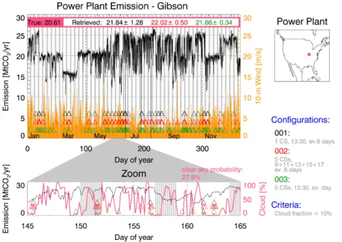
Local Time Ascending Node (LTAN) of 13:30 (01:30 p.m.). This orbit was simulated us-ing Satellite Tool Kit (STK, http://www.agi.com/products/by-product-type/applications/ stk/). We define this as configuration 001, where global coverage is achieved approx-imately every 5 days (see Fig. 3, top panel). Configuration 002 is an extension of configuration 001. It has 5 CarbonSat satellites that also have the same orbit charac-5

teristics but with LTANs that are two hours apart. Global coverage is also achieved in approximately 5 days (see Fig. 3, middle panel). Lastly, configuration 003 has also 5 CarbonSat satellites all having an LTAN of 13:30 and are one day apart, which means that global coverage will be achieved every day (Fig. 3, lowest panel). Table 1 sum-marizes the characteristics of the diﬀ_{erent CarbonSat configurations. For visual clarity,}

10

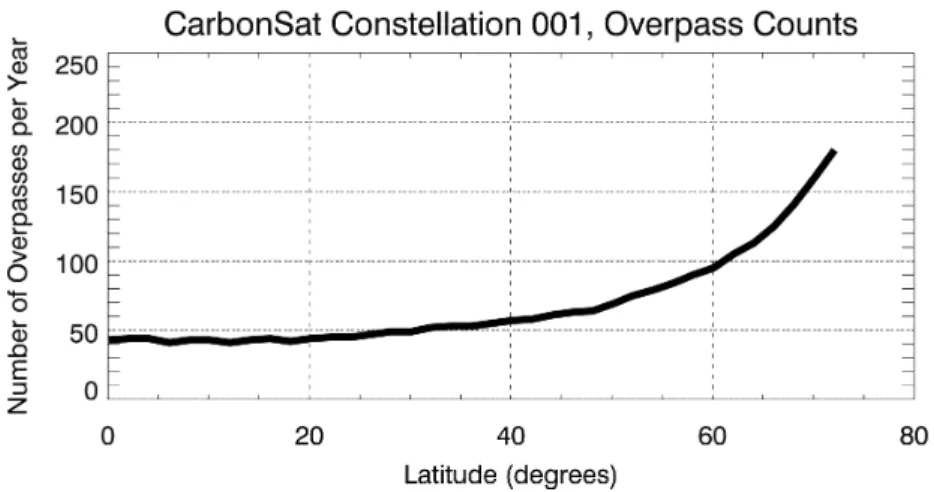
we also plotted the expected number of CarbonSat overpasses per year as a function of latitude in Fig. 4. Power plants in the mid-latitudes, where most industrialized na-tions are located, will have about 50 overpasses per year. The clear-sky probabilities obtained from MODIS can help provide an approximation of the cloud-free measure-ments over a target (Fig. 5), so that from the number of theoretical overpasses (Fig. 4), 15

one can deduce the expected cloud free measurements just by looking at the MODIS dataset. However, care must be taken in doing the interpretation because very thin cirrus clouds are sometimes hard to detect with MODIS (Reuter et al., 2009).

2.4 Estimation of errors

Bovensmann et al. (2010) analyzed and quantified several error sources arising from 20

the retrieval of power plant CO₂ emissions. From a single CarbonSat overpass, they studied errors due to aerosols, instrument noise, advection and mixing. They found that the random error arising from instrument noise primarily depends on near-surface wind speed (∼1 MtCO₂ per 1 m s−1) because with increasing wind speed, the ampli-tude of the CO₂emission plume gets smaller so that instrument noise becomes more 25

important. They also found that neglecting enhanced aerosol concentrations in the power plant plume may result in errors in the range of 0.2–2.5 MtCO₂yr−1

(11)

AMTD

4, 5147–5182, 2011

emissions

Title Page

Tables Figures

◭ ◮

Back Close

Full Screen / Esc

Discussion

P

a

per

|

Dis

cussion

P

a

per

|

Discussion

P

a

per

|

Discussio

n

P

a

per

|

on power plant aerosol emission.

In this study, we focus on systematic errors of inferred annual emissions arising from sparse sampling and on the wind speed dependent statistical (random) error, which can be interpreted as the CO₂ emission detection limit for power plants and other strong CO₂point sources as mentioned in Bovensmann et al. (2010).

5

The total error of the derived annual power plant emissions is a combination of sam-pling error (systematic error) and random error (due to wind speed). Within this study, we are able to quantify both error components because the power plant emissions are assumed to be known. Whereas in reality, only the random error is known and the sam-pling error component would have to be estimated e.g. from the results of the study at 10

hand.

First, we determine the systematic errors due to sparse sampling. We simulated satellite overpasses for each power plant location. For each overpass, we took the power plant’s reported CO₂emission (at 13:00 local time) and assume that CarbonSat would measure the same amount of CO₂ without errors. Since the power plant load 15

and the corresponding CO₂ emissions vary with time, this sparse sampling at fixed time intervals is expected to yield a bias in the CO₂ annual emission estimate. The sparse sampling will be further reduced depending on the cloud cover at the power plant location because we assume that CarbonSat will not be able to measure during scenarios with a cloud fraction of more than 10 % in a 32×32 km2area (i.e. we require 20

an essentially cloud-free scene around the power plant in order to observe most of the CO₂emission plume. So simulated overpasses with cloud contamination of>10 % are flagged and considered as “no measurement”. The estimated annual CO₂emission measured by CarbonSat ( ˆE) over a certain power plant is then calculated as:

ˆ E=1

n

X

j=0

E_jtN (1)

(12)

AMTD

4, 5147–5182, 2011

emissions

Title Page

Tables Figures

◭ ◮

Back Close

Full Screen / Esc

Discussion

P

a

per

|

Dis

cussion

P

a

per

|

Discussion

P

a

per

|

Discussio

n

P

a

per

E_jtis the “true” CO₂emitted by a power plant at the overpass hourj(reported values in tons CO₂/hr),Nis the number of hours in a year andnthe actual number of overpass hours. The “true” power plant annual emission (ET) is the sum of all the hourly-reported CO₂for the whole year:

ET= N

X

i=₀

E_it (2)

5

The bias is simply the diﬀ_{erence between ˆ}_E _{(the annual emission as retrieved from}

CarbonSat) andET(the true annual CO₂ emission) (see results shown in Fig 6-9 for diﬀ_{erent CarbonSat scenarios applied to selected power plants, as discussed in detail}

below).

As mentioned before, we assume that the error of each simulated measurement is 10

only dependent on the wind speed at the time of the satellite pass over the power plant location, neglecting other possible error sources. In line with the findings of Bovensmann et al., 2010, we also assume that the measurement random errors are linear, i.e. we conservatively assigned a 1.0-MtCO₂yr−1 error for every 1-m/s wind speed (Bovensmann et al., 2010 showed that the error is to a good approximation 15

0.8 MtCO₂yr−1_{per 1 m s}−1_{wind speed) .}

To calculate the random errors of ˆE, we use a general method already shown by Reuter et al. (2010) to estimate the total error of an averaged quantity as a combina-tion of the measurement error and the sampling error without knowledge on the true average value of the distribution. We write the Jacobians of ˆE as:

20

KEˆ=

1 n,...,

1 n

(13)

AMTD

4, 5147–5182, 2011

emissions

Title Page

Tables Figures

◭ ◮

Back Close

Full Screen / Esc

Discussion

P

a

per

|

Dis

cussion

P

a

per

|

Discussion

P

a

per

|

Discussio

n

P

a

per

|

wherenis the dimension of ˆE (equal to the number of overpasses). The error covari-ance matrixS_Eis given by

SE=



 

Var(E₁) ··· Cov(E₁,E_n) ..

. . .. ... Cov(E_n,E₁) ··· Var(E_n)





 (4)

The diagonal terms ofS_Erepresent the errors (squared) derived from the wind speed at the time of the overpass at the power plant location. We assume that the data are 5

independent so that the oﬀ_{diagonals of}_S_E_{are zero. The variance of the estimate ˆ}_E_is

then calculated as:

V ar( ˆE)=_K_ˆ

ESEKT_E_ˆ (5)

3 Results and discussion

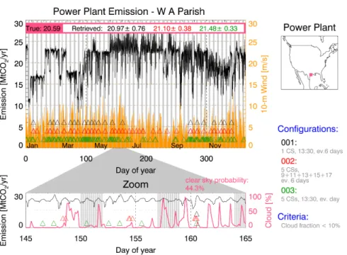
Figure 6 shows typical hourly emissions of a power plant in Arizona, USA (Navajo 10

Generating Station) for 2008. The top panel of Fig. 6 shows the systematic error cal-culations obtained from the diﬀ_{erent configurations. For each overpass, a}

measure-ment consists of two values, the estimated emission (assumed to be free of systematic errors) and its wind speed-dependent statistical uncertainty (random error). The es-timated annual emission as inferred from the CarbonSat observations is the mean of 15

the measured emissions of all overpasses, i.e. ˆE. The variance of ˆE follows from Eq. (5). As can be seen for this example (see bar on top), the true emission is 20.43 MtCO₂yr−1_{. For configuration 001 the estimated emission is 21.28}

±0.65 MtCO₂yr−1. For configuration 002, the retrieved value would be 21.10±0.28 MtCO₂yr−1 and for configuration 003: 21.23±0.23 MtCO₂yr−1. As expected, systematic errors occur due 20

(14)

AMTD

4, 5147–5182, 2011

emissions

Title Page

Tables Figures

◭ ◮

Back Close

Full Screen / Esc

Discussion

P

a

per

|

Dis

cussion

P

a

per

|

Discussion

P

a

per

|

Discussio

n

P

a

per

marginally. The reason for this is that, in this example, the CO₂ emissions during day do not vary so much (therefore one sample per day is suﬃ_{cient). Also, the day to day}

variations are small, even when comparing weekdays with weekends (grey shaded ar-eas). The Navajo generating station partially supplies the city of Los Angeles (∼900 km away) as well as the city of Las Vegas (www.srpnet.com/about/stations/navajo.aspx). 5

These are two cities that have a huge electricity demand for air-conditioning, leading to a large day-night diﬀ_{erence in power demand, especially in the summer months.}

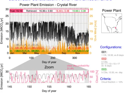
Fig-ures 7–9 show similar plots for three other power plants. These plants are only some of the highest CO₂-emitting power plants in the US. As can be seen, the characteris-tics of the hourly emissions are diﬀ_{erent for each power plant. For example, for the}

10

power plant Crystal River (Fig. 9), the day/night contrast is substantial. Since power consumption at night is usually lower than during the day, this leads to systematically higher retrieved values for all configurations. We have also compared the diﬀ_erences

in emissions during cloudy and clear skies. Although there is a link between temper-ature and electrical consumption (Petron et al., 2008), we found that the diﬀ_{erence in}

15

emissions during cloudy and clear days is very small (∼3 %) when averaged over all the power plants we investigated.

The statistics for all power plants are shown in Fig. 10. It shows the results for power plants emitting more than or equal to 5 MtCO₂yr−1_{in the US (157 power plants).}

The results can be summarized as follows: The systematic error of the annual CO₂ 20

emissions of all power plants in the US emitting more than or equal to 5 MtCO₂yr−1 as obtained from one CarbonSat due to sparse time sampling is less than 4.9 % for 50 % of the power plants and less than 12.4 % for 90 % of all power plants. Using a combination of 5 CarbonSats essentially does not result in a large reduction of this error. However, the smallest systematic error is obtained with configuration 003. This 25

is because the day-to-day variability is larger (e.g. diﬀ_{erences between weekdays and}

(15)

AMTD

4, 5147–5182, 2011

emissions

Title Page

Tables Figures

◭ ◮

Back Close

Full Screen / Esc

Discussion

P

a

per

|

Dis

cussion

P

a

per

|

Discussion

P

a

per

|

Discussio

n

P

a

per

|

The statistical (or random) error of the estimated emissions using one CarbonSat is less than 6.7 % for 50 % of the power plants (≥5 MtCO₂yr−1) and less than 13.0 % for 90 % of all power plants (≥5 MtCO₂yr−1) . This improves by approximately a factor of two if 5 CarbonSats are used (configuration 002 & 003). Qualitatively, the same conclusions can be drawn if all power plants emitting more than 1 MtCO₂yr−1are used 5

(see Table 2) or all those emitting more than 10 MtCO₂yr−1.

By contrast, mass emission rates reported by Electric Generation Utilitiy (EGU) power plants in the US equipped with CEMS are reported to have an accuracy of±14 % or better (Peischl et al., 2010). In another study, Ackerman and Sundquist (2008) re-ported that the absolute diﬀ_{erences between estimates of emissions from individual}

10

power plants can be of up to 25 % (EPA eGRID vs EIA datasets). Moreover, the CO₂ calculation approach used in the European Trading Scheme was reported to have a bias of up to 20 % (Evans et al., 2009).

Regarding changes in annual CO₂ emissions, it is also important to know up to what extent CarbonSat would be able to detect reductions or increases in emissions 15

of power plants. Therefore, we extend our method to 14 yr of emissions data reported by three selected power plants. Figure 11 shows the annual variability of CO₂ emis-sions from the Springerville generating station as well as the estimated annual CO₂ emissions from three diﬀ_{erent CarbonSat constellation configurations (color-coded). It}

can be seen that CarbonSat captures the changes in emissions, for example, the huge 20

increase in 2006 after the company has installed a third unit (418 MW). The decrease in emissions from 2008–2009, probably as a consequence of a fire at the station, is also detected. In December 2009, Unit 4 (400 MW) became operational, this explains the increased emissions in the following year, which is also captured by CarbonSat. For information on the power plant and its history, see also: www.tucsonelectric.com/ 25

(16)

AMTD

4, 5147–5182, 2011

emissions

Title Page

Tables Figures

◭ ◮

Back Close

Full Screen / Esc

Discussion

P

a

per

|

Dis

cussion

P

a

per

|

Discussion

P

a

per

|

Discussio

n

P

a

per

is the implementation of the renewable energy policy by the Los Angeles Department of Water and Power (LADWP). In 2010, LADWP has achieved its goal of reducing CO₂emissions (∼2.5 MtCO₂yr−1) by sourcing up to 20 % of its power from green and renewable energy (www.ladwp.com/ladwp/cms/ladwp04197.jsp). Figure 13 shows an example of a somewhat steady annual CO₂ emission from a power plant (Coronado 5

generating station in Arizona). The agreement between the reported CO₂ emissions and the simulated CarbonSat measurements are quite good, especially in the years after 1998. Figures 11–13 indicate that CarbonSat has the potential to be an important tool for monitoring power plant annual emission changes.

4 Summary and conclusions

10

From the orbit, swath and measurement characteristics of the proposed CarbonSat satellite instrument, we have characterized errors arising from power plant CO₂ sions monitoring. We quantified two types of errors: (i) systematic error of annual emis-sions arising from sparse sampling of the power plant’s emission and (ii) wind speed-dependent random errors caused by instrument detector noise (Bovensmann et al., 15

2010). We used a database containing hourly CO₂ emissions from US power plants and combined this with reanalyzed meteorological conditions (wind, cloud cover). Two CarbonSat constellations, both comprising of 5 CarbonSat satellites, were also stud-ied. We have shown that, despite the variability of the power plant emissions and the limited satellite overpasses, one CarbonSat can verify reported annual CO₂emissions 20

from large power plants (≥5 MtCO₂yr−1) with a systematic (sampling) error of∼4.9 % or better for 50 % of all the power plants and ∼12.4 % or better for 90 % of all the power plants. Using a combination of 5 CarbonSats improves the random errors by approximately a factor of two, but essentially does not result in a large reduction of the systematic error. The reason is that the systematic error caused by sparse time 25

(17)

AMTD

4, 5147–5182, 2011

emissions

Title Page

Tables Figures

◭ ◮

Back Close

Full Screen / Esc

Discussion

P

a

per

|

Dis

cussion

P

a

per

|

Discussion

P

a

per

|

Discussio

n

P

a

per

|

Two configurations of 5-CarbonSat constellations have been investigated. One achieves global coverage every day but only at fixed local times (configuration 003). The other performs measurements every two hours but only achieved global coverage after 5 days (configuration 002). For the purpose of power plant emissions monitoring, both configurations are similar but configuration 003 achieves somewhat smaller sys-5

tematic errors. Configuration 002 might be advantageous for observing the daily cycle of CO₂, but for other reasons, fast global coverage is important, such as for monitoring important events that only last a few days. Examples of these events are: biomass burning, (mud) volcanic eruptions and sudden release of CH₄ below ice/snow after melting in spring or ice break up (Siberia, Alaska). A constellation of exactly identical 10

CarbonSats in essentially identical orbits has also the advantage of higher accuracy due to better (easier) inter-calibration between the various satellites. For these rea-sons, we therefore conclude that the preferred configuration is configuration 003, i.e. the one which achieved global coverage within the shortest time period (even if only one measurement per day can be taken). Furthermore, if the strict reporting rules im-15

posed on US power plants are implemented in other countries, CarbonSat can serve as an independent verification system by checking the reported emissions at the hours of the overpasses. By comparing the routinely reported power plant emissions and the coincident CarbonSat measurements for that hour, the systematic errors from the sparse sampling will not be a significant error source. Instead, other error sources such 20

as aerosols, wind speeds, albedo, etc. will be more important. These can be improved through retrieval algorithm development.

Acknowledgements. We would like to acknowledge the Wirtschaftsfoerderung Bremen (WFB) for funding and supporting the CarbonSat constellation study. We also acknowledge NASA and the teams involved in producing the MODIS data. NARR data was provided by the 25

(18)

AMTD

4, 5147–5182, 2011

emissions

Title Page

Tables Figures

◭ ◮

Back Close

Full Screen / Esc

Discussion

P

a

per

|

Dis

cussion

P

a

per

|

Discussion

P

a

per

|

Discussio

n

P

a

per

References

Ackerman, K. V. and Sundquist, E. T.: Comparison of Two U.S. Power-Plant Carbon Dioxide Emissions Data Sets, Environ. Sci. Technol., 42, 5688–5693, 2008. 5161

Amediek, A., Fix, A., Ehret, G., Caron, J., and Durand, Y.: Airborne lidar reflectance measure-ments at 1.57 µm in support of the A-SCOPE mission for atmospheric CO2, Atmos. Meas.

5

Tech., 2, 755–772, doi:10.5194/amt-2-755-2009, 2009. 5151

Boesch, H., Baker, D., Connor, B. J., Crisp, D., and Miller, C.: Global Characterization of CO₂ Column Retrievals from Shortwave-Infrared Satellite Observations of the Orbiting Carbon Observatory-2 Mission, Remote Sens., 3, 270–34, doi:10.3390/rs3020270, 2011. 5151 Bovensmann, H., Burrows, J. P., Buchwitz, M., Frerick, J., No ¨el, S., Rozanov, V. V., Chance, 10

K. V., and Goede, A.: SCIAMACHY – Mission Objectives and Measurement Modes, J. At-mos. Sci., 56, 127–150, 1999. 5151

Bovensmann, H., Buchwitz, M., Burrows, J., Reuter, M., Krings, T., Gerilowski, K., Schneising, O., Heymann, J., Tretner, A., and Erzinger, J.: A remote sensing technique for global monitor-ing of power plant CO2emissions from space and related applications, Atmos. Meas. Tech.,

15

3, 781–811, doi:10.5194/amt-3-781-2010, 2010. 5148, 5152, 5154, 5156, 5157, 5158, 5162 Br ´eon, F.-M. and Ciais, P.: Spaceborn remote sensing of greenhouse gas concentrations, C. R.

Geoscience, doi:10.1016/j.crte.2009.09.012, 2009. 5151

Buchwitz, M., Schneising, O., Burrows, J. P., Bovensmann, H., Reuter, M., and Notholt, J.: First direct observation of the atmospheric CO2year-to-year increase from space, Atmos. Chem.

20

Phys., 7, 4249–4256, doi:10.5194/acp-7-4249-2007, 2007. 5151

Burrows, J. P., H ¨olzle, E., Goede, A. P. H., Visser, H., and Fricke, W.: SCIAMACHY – Scan-ning Imaging Absorption Spectrometer for Atmospheric Chartography, Acta Astronautica, 35, 445–451, 1995. 5151

Ch ´edin, A., Hollingsworth, A., Scott, N. A., Serrar, S., Crevoisier, C., and Armante, 25

R.: Annual and seasonal variations of atmospheric CO2, N2O and CO

concentra-tions retrieved from NOAA/TOVS satellite observaconcentra-tions, Geophys. Res. Lett., 29, 1269, doi:10.1029/2001GL014082, 2002. 5151

Ch ´edin, A., Serrar, S., Scott, N. A., Crevoisier, C., and Armante, R.: First global measurement of midtropospheric CO2 from NOAA polar satellites: Tropical zone, J. Geophys. Res., 108,

30

4581, doi:10.1029/2003JD003439, 2003. 5151

(19)

AMTD

4, 5147–5182, 2011

emissions

Title Page

Tables Figures

◭ ◮

Back Close

Full Screen / Esc

Discussion

P

a

per

|

Dis

cussion

P

a

per

|

Discussion

P

a

per

|

Discussio

n

P

a

per

|

atmospheric CO2concentrations from a high resolution fossil fuel CO2emissions inventory,

Tellus, 62B, 506–511, doi:10.1111/j.1600-0889.2010.00480.x, 2010. 5150

Crevoisier, C., Ch ´edin, A., Matsueda, H., Machida, T., Armante, R., and Scott, N. A.: First year of upper tropospheric integrated content of CO2 from IASI hyperspectral infrared observa-tions, Atmos. Chem. Phys., 9, 4797-4810, doi:10.5194/acp-9-4797-2009, 2009. 5151 5

Crisp, D., Atlas, R. M., Br ´eon, F.-M., Brown, L. R., Burrows, J. P., Ciais, P., Connor, B. J., Doney, S. C., Fung, I. Y., Jacob, D. J., Miller, C. E., O’Brien, D., Pawson, S., Randerson, J. T., Rayner, P., Salawitch, R. S., Sander, S. P., Sen, B., Stephens, G. L., Tans, P. P., Toon, G. C., Wennberg, P. O., Wofsy, S. C., Yung, Y. L., Kuang, Z., Chudasama, B., Sprague, G., Weiss, P., Pollock, R., Kenyon, D., and Schroll, S.: The Orbiting Carbon Observatory (OCO) 10

mission, Adv. Space Res., 34, 700–709, 2004. 5151

Ellerman, D. A. and Buchner, B. K.: The European Union Emissions Trading Scheme: Origins, Allocation, and Early Results, Review of Environmental Economics and Policy, 1, 66–87, doi:10.1093/reep/rem003, 2007. 5150

Engelen, R. J. and McNally, A. P.: Estimating atmospheric CO2from advanced infrared satellite

15

radiances within an operational 4D-Var data assimilation system: Results and validation, J. Geophys. Res., 109, D18305, doi:10.1029/2005JD005982, 2005. 5151

Engelen, R. J. and Stephens, G. L.: Information content of satellite sounding measurements with respect to CO₂, J. Appl. Meteorol., 43, 373–378, 2004. 5151

Engelen, R. J., Andersson, E., Chevallier, F., Hollingsworth, A., Matricardi, M., McNally, A. P., 20

Th ´epaut, J.-N., and Watts, P. D.: Estimating atmospheric CO₂from advanced infrared satel-lite radiances within an operational 4D-Var data assimilation system: Methodology and first results, J. Geophys. Res., 109, D19309, doi:10.1029/2004JD004777, 2004. 5151

Evans, S., Deery, S., and Bionsa, J.: How Reliable are GHG Combustion Calculations and Emission Factors?, Presented at the CEM 2009 Conference, Milan, Italy, 2009. 5150, 5161 25

Forster, P., Ramaswamy, V., Artaxo, P., Berntsen, T., Betts, R., Fahey, D., Haywood, J., Lean, J., Lowe, D., Myhre, G., Nganga, J., Prinn, R., Raga, G. M. S., and Dorland, R. V.: Changes in Atmospheric Constituents and in Radiative Forcing. In: Climate Change 2007: The Physical Science Basis. Contribution of Working Group I to the Fourth Assessment Report of the In-tergovernmental Panel on Climate Change, Cambridge University Press, Cambridge, United 30

Kingdom and New York, NY, USA, 2007. 5149

(20)

SCIA-AMTD

4, 5147–5182, 2011

emissions

Title Page

Tables Figures

◭ ◮

Back Close

Full Screen / Esc

Discussion

P

a

per

|

Dis

cussion

P

a

per

|

Discussion

P

a

per

|

Discussio

n

P

a

per

MACHY: Trends and variability, J. Geophy. Res., 116, D04302, doi:10.1029/2010JD014849, 2011. 5151

Gurney, K. R., Law, R. M., Denning, A. S., Rayner, P. J., Baker, D., Bousquet, P., Bruhwiler, L., Chen, Y.-H., Ciais, P., Fan, S., Fung, I. Y., Gloor, M., Heimann, M., Higuchi, K., John, J., Maki, T., Maksyutov, S., Masarie, K., Peylin, P., Prather, M., Pak, B. C., Randerson, 5

J., Sarmiento, J., Taguchi, S., Takahashi, T., and Yuen, C.-W.: Towards robust regional esti-mates of CO2sources and sinks using atmospheric transport models, Nature, 415, 626–630,

doi:10.1038/415626a, 2002. 5149

Gurney, K. R., Chen, Y.-H., Maki, T., Kawa, S. R., Andrews, A., and Zhu, Z.: Sensitivity of atmospheric CO2inversions to seasonal and interannual variations in fossil fuel emissions,

10

J. Geophy. Res., 110, D10308, doi:10.1029/2004JD005373, 2005. 5150

Hamazaki, T., Kaneko, Y., and Kuze, A.: Carbon dioxide monitoring from the GOSAT satellite, Proceedings XXth ISPRS conference, Istanbul, Turkey, 12–23 July 2004, 2004. 5151 Krings, T., Gerilowski, K., Buchwitz, M., Reuter, M., Tretner, A., Erzinger, J., Heinze, D.and

Bur-rows, J. P., and Bovensmann, H.: MAMAP – a new spectrometer system for column-15

averaged methane and carbon dioxide observations from aircraft: retrieval algorithm and first inversions for point source emission rates, Atmos. Meas. Tech. Discuss., 4, 2207–2271, doi:10.5194/amtd-4-2207-2011, 2011. 5152

Kuang, Z., Margolis, J., Toon, G., Crisp, D., and Yung, Y.: Spaceborne measurements of atmo-spheric CO₂by high-resolution NIR spectrometry of reflected sunlight: an introductory study, 20

Geophy. Res. Lett., 29, 1716, doi:10.1029/2001GL014298, 2002. 5151

Kulawik, S. S., Jones, D. B. A., Nassar, R., Irion, F. W., Worden, J. R., Bowman, K. W., Machida, T., Matsueda, H., Sawa, Y., Biraud, S. C., Fischer, M. L., and Jacobson, A. R.: Characteri-zation of Tropospheric Emission Spectrometer (TES) CO2for carbon cycle science, Atmos.

Chem. Phys., 10, 5601–5623, doi:10.5194/acp-10-5601-2010, 2010. 5151 25

Kuze, A., Suto, H., Nakajima, M., and Hamazaki, T.: Thermal and near infrared sensor for carbon observation Fourier-transform spectrometer on the Greenhouse Gases Observing Satellite for greenhouse gases monitoring, Appl. Opt., 48, 6716–6733, 2009. 5151

Marland, G.: Uncertainties in accounting for CO2 from fossil fuels, J. Ind. Ecol., 12, 136–139,

2008. 5149 30

Marland, G. and Rotty, R. M.: Carbon dioxide emissions from fossil-fuels: A procedure for estimation and results for 1950–1982, Tellus, Ser. B, 36, 232–261, 1984. 5149

(21)

AMTD

4, 5147–5182, 2011

emissions

Title Page

Tables Figures

◭ ◮

Back Close

Full Screen / Esc

Discussion

P

a

per

|

Dis

cussion

P

a

per

|

Discussion

P

a

per

|

Discussio

n

P

a

per

|

A., Rayner, P., Jacob, D. J., Suntharalingam, P., Jones, D. B. A., Denning, A. S., Nicholls, M. E., Doney, S. C., Pawson, S., Boesch, H., Connor, B. J., Fung, I. Y., O’Brien, D., Salawitch, R. J., Sander, S. P., Sen, B., Tans, P., Toon, G. C., Wennberg, P. O., Wofsy, S. C., Yung, Y. L., and Law, R. M.: Precision requirements for space-basedXCO₂data, J. Geophys. Res., 112, D10314, doi:10.1029/2006JD007659, 2007. 5151

5

Oda, T. and Maksyutov, S.: a very high-resolution (1kmx 1km) global fossil fuesl CO₂emission inventory derived using a point source database and satellite observations of nighttime lights, Atmos. Chem. Phys., 11, 543–556, doi:10.5194/acp-11-543-2011, 2011. 5149

Palmer, P. I. and Rayner, P.: Atmospheric science: failure to launch, Nature Geosci, 2, 247, doi:10.1016/j.atmosres.2008. 05.001, 2009. 5151

10

Peischl, J., Ryerson, B., Holloway, J. S., Parrish, D. D., Trainer, M., Frost, G. J., Aikin, K. C., Brown, S. S., Dub ´e, W. P., Stark, H., and C., F. F.: A top-down analysis of emissions from selected Texas power plants during TexAQS 2000 and 2006, J. Geophy. Res., 115, doi:10.1029/2009JD013527, 2010. 5150, 5153, 5154, 5161

Petron, G., Tans, P., Frost, G., Chao, D., and Trainer, M.: High-resolution emissions of CO2from

15

power generation in the USA, J. Geophy. Res., 113, G04008,, doi:10.1029/2007JG000602, 2008. 5150, 5154, 5160

Reuter, M., Thomas, W., Albert, P., Lockhoﬀ_{, M., Weber, R., Karlsson, K. G., and Fischer,} J.: The CM-SAF and FUB cloud detection schemes for SEVIRI: Validation with synoptic data and initial comparison with MODIS and CALIPSO, J. Appl. Met. Clim., 48, 301–316, 20

doi:10.1175/2008JAMC1982.1, 2009. 5156

Reuter, M., Thomas, W., Mieruch, S., and Hollmann, R.: A Method for Estimating the Sampling Error Applied to CM-SAF Monthly Mean Cloud Fractional Cover Data Retrieved From MSG SEVIRI, IEEE T. Geosci. Remote, 48, 2469–2481, doi:10.1109/TGRS.2010.2041240, 2010. 5158

25

(22)

AMTD

4, 5147–5182, 2011

emissions

Title Page

Tables Figures

◭ ◮

Back Close

Full Screen / Esc

Discussion

P

a

per

|

Dis

cussion

P

a

per

|

Discussion

P

a

per

|

Discussio

n

P

a

per

Table 1.Diﬀ_{erent CarbonSat configurations.}

Configuration ID Number of Satellites LTAN Global Coverage

001 1 13:30 after 5 days

002 5 9:30,11:30,13:30,15:30:17:30 after 5 days

(23)

AMTD

4, 5147–5182, 2011

emissions

Title Page

Tables Figures

◭ ◮

Back Close

Full Screen / Esc

Discussion

P

a

per

|

Dis

cussion

P

a

per

|

Discussion

P

a

per

|

Discussio

n

P

a

per

|

Table 2.Error estimates on annual power plant (PP) emissions from three diﬀ_{erent CarbonSat} configurations.

Power Plant (PP) Emissions and Associated Errors from CarbonSat Estimates (in %)

Error Type Power Plant Sample Size

≥1MtCO2yr

−1

≥5MtCO2yr

−1

≥10MtCO2yr

−1 Configuration ID Configuration ID Configuration ID 001 002 003 001 002 003 001 002 003

Systematic 50 % of all PP ≤6.1 ≤5.7 ≤5.6 ≤4.9 ≤4.3 ≤3.9 ≤4.1 ≤4.5 ≤3.8 90 % of all PP ≤17.4 ≤16.6 ≤17.6 ≤12.4 ≤12.3 ≤10.2 ≤10.9 ≤8.9 ≤9.6

(24)

AMTD

4, 5147–5182, 2011

emissions

Title Page

Tables Figures

◭ ◮

Back Close

Full Screen / Esc

Discussion

P

a

per

|

Dis

cussion

P

a

per

|

Discussion

P

a

per

|

Discussio

n

P

a

per

Fig. 1.Hourly CO2emissions from four selected power plants in the US as reported to the EPA.

For consistency, the hourly CO2emissions (in tons CO2hr

−1

) were converted to MtCO2yr

−1

(25)

AMTD

4, 5147–5182, 2011

emissions

Title Page

Tables Figures

◭ ◮

Back Close

Full Screen / Esc

Discussion

P

a

per

|

Dis

cussion

P

a

per

|

Discussion

P

a

per

|

Discussio

n

P

a

per

|

Fig. 2. Diurnal cycle of CO2emissions summed over all power plants (PP) in the US emitting

more that 1.0 MtCO2yr

−1

(26)

AMTD

4, 5147–5182, 2011

emissions

Title Page

Tables Figures

◭ ◮

Back Close

Full Screen / Esc

Discussion

P

a

per

|

Dis

cussion

P

a

per

|

Discussion

P

a

per

|

Discussio

n

P

a

per

(27)

AMTD

4, 5147–5182, 2011

emissions

Title Page

Tables Figures

◭ ◮

Back Close

Full Screen / Esc

Discussion

P

a

per

|

Dis

cussion

P

a

per

|

Discussion

P

a

per

|

Discussio

n

P

a

per

|

(28)

AMTD

4, 5147–5182, 2011

emissions

Title Page

Tables Figures

◭ ◮

Back Close

Full Screen / Esc

Discussion

P

a

per

|

Dis

cussion

P

a

per

|

Discussion

P

a

per

|

Discussio

n

P

a

per

(29)

AMTD

4, 5147–5182, 2011

emissions

Title Page

Tables Figures

◭ ◮

Back Close

Full Screen / Esc

Discussion

P

a

per

|

Dis

cussion

P

a

per

|

Discussion

P

a

per

|

Discussio

n

P

a

per

|

Fig. 6. (top panel) CO2 emissions of a power plant in Arizona, USA (Navajo generating

sta-tion) reported to the EPA for 2008 (black lines). The color-coded triangles represent simulated overpasses for three diﬀ_{erent CarbonSat configurations (001–003, see Table 1) during clear} sky conditions (defined as less than 10 % cloud cover in a 32×32 km area near the position of the power plant and its surroundings). Weekends are indicated by the gray shaded areas. The second y-axis represent the wind speeds (yellow, superimposed). The “true” value of 20.43 (in MtCO2yr

−1

) is simply the sum of the reported CO2for this year. The “retrieved” values of 21.28,

21.10, 21.23 and the corresponding 1-sigma errors (in MtCO2yr

−1

(30)

AMTD

4, 5147–5182, 2011

emissions

Title Page

Tables Figures

◭ ◮

Back Close

Full Screen / Esc

Discussion

P

a

per

|

Dis

cussion

P

a

per

|

Discussion

P

a

per

|

Discussio

n

P

a

per

(31)

AMTD

4, 5147–5182, 2011

emissions

Title Page

Tables Figures

◭ ◮

Back Close

Full Screen / Esc

Discussion

P

a

per

|

Dis

cussion

P

a

per

|

Discussion

P

a

per

|

Discussio

n

P

a

per

|

(32)

AMTD

4, 5147–5182, 2011

emissions

Title Page

Tables Figures

◭ ◮

Back Close

Full Screen / Esc

Discussion

P

a

per

|

Dis

cussion

P

a

per

|

Discussion

P

a

per

|

Discussio

n

P

a

per

(33)

AMTD

4, 5147–5182, 2011

emissions

Title Page

Tables Figures

◭ ◮

Back Close

Full Screen / Esc

Discussion

P

a

per

|

Dis

cussion

P

a

per

|

Discussion

P

a

per

|

Discussio

n

P

a

per

|

Fig. 10.Error analysis for diﬀ_{erent CarbonSat configurations, done for power plants with} emis-sions of more than or equal to 5 MtCO2yr

−1

(34)

AMTD

4, 5147–5182, 2011

emissions

Title Page

Tables Figures

◭ ◮

Back Close

Full Screen / Esc

Discussion

P

a

per

|

Dis

cussion

P

a

per

|

Discussion

P

a

per

|

Discussio

n

P

a

per

(35)

AMTD

4, 5147–5182, 2011

emissions

Title Page

Tables Figures

◭ ◮

Back Close

Full Screen / Esc

Discussion

P

a

per

|

Dis

cussion

P

a

per

|

Discussion

P

a

per

|

Discussio

n

P

a

per

|

(36)

AMTD

4, 5147–5182, 2011

emissions

Title Page

Tables Figures

◭ ◮

Back Close

Full Screen / Esc

Discussion

P

a

per

|

Dis

cussion

P

a

per

|

Discussion

P

a

per

|

Discussio

n

P

a

per