Nonadditive entropy and nonextensive statistical mechanics - An overview after 20 years
Constantino Tsallis
Centro Brasileiro de Pesquisas F´ısicas and National Institute of Science and Technology for Complex Systems Rua Xavier Sigaud 150, 22290-180 Rio de Janeiro, Brazil
and Santa Fe Institute
1399 Hyde Park Road, Santa Fe, NM 87501, USA
(Received on 17 April, 2009)
Statistical mechanics constitutes one of the pillars of contemporary physics. Recognized as such — together with mechanics (classical, quantum, relativistic), electromagnetism and thermodynamics —, it is one of the mandatory theories studied at virtually all the intermediate- and advanced-level courses of physics around the world. As it normally happens with such basic scientific paradigms, it is placed at a crossroads of various other branches of knowledge. In the case of statistical mechanics, the standard theory — hereafter referred to as the
Boltzmann-Gibbs (BG) statistical mechanics— exhibits highly relevant connections at a variety of microscopic, mesoscopic and macroscopic physical levels, as well as with the theory of probabilities (in particular, with the Central Limit Theorem,CLT). In many circumstances, the ubiquitous efects of theCLT, with its Gaussian attractors (in the space of the distributions of probabilities), are present. Within this complex ongoing frame, a possible generalization of theBGtheory was advanced in 1988 (C.T., J. Stat. Phys. 52, 479). The extension of the standard concepts is intended to be useful in those “pathological”, and nevertheless very frequent, cases where the basic assumptions (molecular chaos hypothesis, ergodicity) for applicability of theBGtheory would be violated. Such appears to be, for instance, the case in classical long-range-interacting many-body Hamilto-nian systems (at the so-calledquasi-stationary state). Indeed, in such systems,the maximal Lyapunov exponent vanishesin the thermodynamic limitN→∞. This fact creates a quite novel situation with regard to typicalBG
systems, which generically have apositivevalue for this central nonlinear dynamical quantity. This peculiarity has sensible effects at all physical micro-, meso- and macroscopic levels. It even poses deep challenges at the level of theCLT. In the present occasion, after 20 years of the 1988 proposal, we undertake here an overview of some selected successes of the approach, and of some interesting points that still remain as open questions. Various theoretical, experimental, observational and computational aspects will be addressed.
Keywords: Nonadditive entropy, Nonextensive statistical mechanics, Complex systems, Nonlinear dynamics
1. INTRODUCTION
Statistical mechanics indeed constitutes one of the pillars of contemporary physics. As such — together with mechan-ics (classical, quantum, relativistic), electromagnetism and thermodynamics —, it is one of the basic theories universally studied at intermediate and advanced levels in physics. As it happens with such grounding scientific paradigms, it plays a central role in various other branches of knowledge, includ-ing chemistry, biology, mathematics, computational sciences, to name but the most obvious ones. The standard theory — hereafter referred to as the Boltzmann-Gibbs (BG) statisti-cal mechanics— exhibits many connections at a variety of microscopic(mechanics, classical and quantum field theory, electrodynamics, nonlinear dynamical systems, gravitation), mesoscopic (Langevin, master equation, Fokker-Planck ap-proaches, Vlasov equation) andmacroscopic (thermodynam-ics, science of complexity) physical descriptions, as well as with mathematics (theory of probabilities, Central Limit The-orem,CLT).
Those physical approaches that are usually consideredfrom first principles inescapable involve up to four independent and universal physical constants, namely the Planck constant (h), the velocity of light in vacuum (c), the gravitation con-stant (G), and the Boltzmann constant (kB). All presently known physical units can be expressed as multiplicative ex-pressions of powers of these four constants. Naturally, op-timally formulated mathematics involve none of these con-stants, i.e., the exponents of all those powers vanish (which legitimates the common usage of units such thath=c=G=
kB=1). The constantkBalways appears, in one way or an-other, in statistical mechanics (e.g., in the laws of the ideal classical gas). In many instances, it is accompanied by the constanth(e.g., in Fermi-Dirac and Bose-Einstein statistics). The constantccan also be in the party (e.g., in the various forms expressing the laws of the black-body radiation). The constantGaccompanieskBwhenever gravitation is taken into account (e.g., the variation of air density of the Earth atmo-sphere as a function of height, due to the gravitational mass attraction). Finally, all four constantsh,c,GandkBcan be simultaneously present (e.g., in quantum gravitation thermo-statistical expressions such as the entropy of a black-hole). In many of these and other circumstances, the efects of theCLT, with its Gaussian attractors (in the space of the distributions of probabilities), show up.
FIG. 1: Physical structure at thek−B1=0 plane. The full diagram involves four universal constants, and corresponds to successively embedded tetrahedra. At the center of the tetrahedron we have the caseG=c−1=h=kB−1=0, and the overall tetrahedron corresponds toG>0,c−1>0,h>0,k−B1>0 (statistical mechanics of quantum gravity).
The above considerations are consistent with the fact that Planck introduced [1, 2] (see also [3–8]) four natural units for length,mass,time, andtemperature, namely
unit o f length = r
hG
c3 =4.13×10− 33cm(1)
unit o f mass =
r
hc
G =5.56×10 −5g
(2)
unit o f time =
r
hG
c5 =1.38×10− 43s
(3)
unit o f temperature = 1
kB r
hc5
G =3.50×10
32K (4)
There is no need to add to this list the elementary elec-tric chargee. Indeed, it is related to the already mentioned constants through thefine-structure constantα≡2πe2/hc=
1/137.035999...
In 1988, a generalization of theBGtheory was proposed [9], inspired by the structure of multifractals. It is based on thenonadditive entropy Sq(q∈
R
), to be defined in the next Section, and is currently referred to asnonextensive statistical mechanics; it recovers the (additive)BGentropy and its asso-ciated statistical mechanics as theq=1 particular instance. The extension of the standard concepts focuses on the fre-quent “pathological” cases where the basic assumptions (e.g., molecular chaos hypothesis, ergodicity) for applicability of theBGtheory are violated. One paradigmatic case concerns classical long-range-interacting many-body Hamiltonian sys-tems (at the so-calledquasi-stationary state). Indeed, in such systems,the maximal Lyapunov exponent vanishesin the ther-modynamic limitN→∞. This fact is completely atypical within theBGscenario. Indeed, most of the dynamical sys-tems that have usually been studied, within the BGtheory, during the last 130 years generically have apositivevalue forthe maximal Lyapunov exponent. This property has impor-tant consequences at physical micro-, meso- and macroscopic levels. Also, it sustains connections with the most important CLT. Last but not least, as we shall soon see, the quantity
(q−1)intriguingly couples to the universal constantkB. In Section 2, we briefly introduce the nonadditive entropy Sq, and its associated statistical mechanics. In Section 3, we show how the indice(s)q are to be determined from micro-or scopic infmicro-ormation; we also describe typical meso-scopic mechanisms that are known to yield nonextensive statistics. In Section 4, we briefly illustrate the ubiquitous emergence of q-Gaussians (in general q-exponentials) in natural, artificial and social systems; consistently we present the q-generalization of the CLT, which can be thought as being the cause of this ubiquity. We finally conclude in Section 5.
2. NONADDITIVE ENTROPY AND NONEXTENSIVE STATISTICAL MECHANICS
The entropic form introduced and studied by Boltzmann, Gibbs, von Neumann, Shannon and many others will from now on be referred to as theBGentropySBG. For the discrete case, it is given by
SBG=−k W
∑
i=1pilnpi, (5)
with
W
∑
i=1pi=1 (pi∈[0,1]), (6)
whereW is the number of possible microscopic states, and k some conventional constant, typically taken to be kB in physics, and unity (or some other convenient dimensionless value) in computational sciences and elsewhere. For the par-ticular case of equal probabilities (i.e.,pi=1/W,∀i), we im-mediately obtain the celebrated formula
SBG=klnW. (7)
The generalization ofSBGproposed in [9] for generalizing
BGstatistical mechanics is the following:
Sq=k
1−∑Wi=1p
q i
q−1 (q∈
R
;S1=SBG). (8) For the particular case of equal probabilities, we obtainSq=klnqW, (9)
where theq-logarithmic functionis defined as follows:
lnqx≡
x1−q−1
1−q (x>0; ln1x=lnx). (10) Its inverse, theq-exponential function, is given by
exq≡[1+ (1−q)x]
1 1−q
where[z]+≡max{z,0}.
The entropy (8) has various predecessors and related en-tropies. The (repeated) references to all these are largely dif-fused in the literature of nonextensive statistical mechanics. A summary can be found in [10].
It is worth mentioning that the entropySqcan be equiva-lently re-written as follows:
Sq=k W
∑
i=1pilnq 1 pi
=−k
W
∑
i=1pqilnqpi=−k W
∑
i=1piln2−qpi (12) If we have twoprobabilistically independentsystemsAand B, i.e. such that p(i jA+B)=pi(A)p(jB),∀(i,j), we immediately verify
Sq(A+B)
k =
Sq(A)
k +
Sq(B)
k + (1−q) Sq(A)
k
Sq(B)
k , (13) hence
Sq(A+B) =Sq(A) +Sq(B) +
(1−q)
k Sq(A)Sq(B). (14) Therefore, forq=1, we recover the well knownadditivityof theBGentropy, i.e.,
SBG(A+B) =SBG(A) +SBG(B), (15) and this is so foranyfinite value ofk. We also see that, for q6=1,Sqisnonadditive. We further see that, forq6=1, ad-ditivity is asymptotically recovered in the limitk→∞. More precisely, it is asymptotically recovered for(1−q)/k→0, which creates a deep relationship between nonextensivity and the limit k→∞. Since the temperature T is accom-panied by k (in the form kT) in any stationary-state dis-tribution and any equation of states involving the tempera-ture, this fact can be seen as the reason which makes the high-temperature asymptotic behavior of all known statis-tics (Boltzmann-Gibbs, Fermi-Dirac, Bose-Einstein, Gentile parastatistics, nonextensive statistics) to be one and the same, essentially the Maxwell-Boltzmann one.
The entropySqcan be, and has been, used in a great vari-ety of situations for natural, artificial and social systems [11]. If the system is a physical one being described by a Hamil-tonian, one can also develop a statistical mechanics ( nonex-tensive statistical mechanics) as follows. Let us illustrate the procedure for the canonical ensemble (the system being in long-standing thermal contact with a large thermostat). We extremizeSqwith constraint (6), and also constraint [12]
h
H
iq≡W
∑
i=1Pi(q)Ei=Uq, (16)
where the{Ei}is the set of eigenvalues associated with the Hamiltonian
H
(and corresponding boundary conditions),Uq is a fixed value characterizing thewidth of the distribution (we note that the width must always be afinitevalue, a prop-erty which isnotguaranteed for the standard mean value, i.e. with probabilities{pi}, ifqhappens to be not close enough to unity), andPi(q)≡ p
q i ∑Wj=1p
q j
(17)
is referred to as theescort distribution. It follows straightfor-wardly that
pi≡ h
Pi(q)i 1
q
∑Wj=1
h
P(jq)i 1
q
. (18)
This optimization procedure yields, for the stationary state,
pi=
e−βq(Ei−Uq) q
∑Wj=1e
−βq(Ej−Uq) q
, (19)
with
βq= β ∑Wj=1p
q j
, (20)
β being the Lagrange parameter associated with constraint (16). Further details, as well as the connections with ther-modynamics, can be seen in [12, 13].
The form of the energy constraint (16), usingPi(q) instead of the usual pi can be understood along various convergent lines. Let us restrict here to mentioning thatboththe norm and the energy constraints are well defined (i.e., correspond-ing tofinitevalues) forqbelow some critical value, and both divergeforqequal or above that value. In the absence of de-generacy, this critical value is q=2 (note that the standard mean value of the energy isfiniteonly up toq=3/2, being infinite forq≥3/2). The use of theq-expectation values such as (16) has been recently criticized in [14]. This critique has been replied in [15, 16]. Further arguments that could sug-gest the use ofq-expectation values can be found in [10], and also in [17–24]. Other arguments that could suggest the use of standard averages can be found in [24–26]. This particular issue is somewhat unclear at the present date. Indeed, in addi-tion to the various apparently contradicting arguments, calcu-lations also exist which suggest the equivalence ofboth pro-cedures (either using, for the energy constraint, averages with {pi}, or using averages with{Pi}whenever the former ones are finite) [12, 27]. To illustrate however a basic point, let us assume that the variablexruns from zero to infinity, and that the energy is proportional toxσ(σ>0). The stationary-state exhibits therefore a probabilityp(x)∝e−qβxσ, hence, asymp-totically forx→∞, p(x)∼x−σ/(q−1). This distribution (i) is normalizable only forq<1+σ(henceq<2 forσ=1, andq<3 forσ=2); (ii) satisfies thathxσiis finite only for q<(1+2σ)/(1+σ)(henceq<3/2 forσ=1, andq<5/3 forσ=2); (iii) satisfies thathxσiqis finite only forq<1+σ, which coincides with the upper bound for normalizability. In other words, if we useq-expectation values, the entire theory is valid up toq=1+σ, whereas if we use standard expecta-tion values, the norm-constraint is mathematically admissible up toq=1+σ, and the energy-constraint is mathematically admissible up to a lower value, namely(1+2σ)/(1+σ).
3. DETERMINING THE INDICESq, AND THE EXTENSIVITY OF THE NONADDITIVE ENTROPYSqFOR
COMPLEX SYSTEMS
3.1. Sets of indicesq
The theory advanced in the previous Section is in principle valid for arbitray values of the indexq. We shall now address the following essential question: For a given specific system or class of systems, how can we determine the values of its indice(s) q?To start, let us point out that, for a given system, not one but a whole family of (possibly infinite countable) indices{q}is to be determined. Let us give a few examples:
qsensitivity : A dissipative one-dimensional (or, say, con-servative two-dimensional) nonlinear dynamical systemx(t)
typically exhibits a sensitivity to the initial conditionsξ≡ lim∆x(0)→0
∆x(t)
∆x(0) of the form
ξ=eλqqsensitivitysensitivity t, (21)
where λqsensitivity is the q-generalized Lyapunov coefficient.
A practical numerical manner for determining it consists in plotting lnqξ(t) versus t for various values of q until a value is found so that, asymptotically in the t →∞ limit, lnqξ(t)∝t. That value of q is qsensitivity, and the slope is λqsensitivity. The two most interesting situations occur for strong
chaos (i.e., when the Lyapunov exponent λ1 is positive), and for weak chaos (at the edge of chaos, whereλ1=0 and
λqsensitivity>0). In the former case we haveqsensitivity=1; in
the latterqsensitivity<1. Although not particularly relevant within the present context,qsensitivity>1 can also occur. Such is the case at double-period and tangent bifurcation critical points.
qentropy production: The phase space of ad-dimensional non-linear dynamical system is partitioned into many W cells. We put, in one of those cells (chosen randomly, or in any other convenient manner),M initial conditions, and then let these points spread around. We define pi(t)≡Mi(t)/M (i=1,2,3, ...,W), whereMi(t)is the number of points within thei-th cell at timet(∑Wi=1Mi(t) =M,∀t). We then calculate, with these{pi(t)}into Eq. (8),Sq(t)/k. We will verify that, for a huge class of nonlinear dynamical systems, a value ofq exists such thatSq(t)∝t. That value ofqisqentropy production, and the slope is theq-generalized Kolmogorov-Sinai-like en-tropy production rateKqentropy production. To be more precise, we
have
lim
t→∞Wlim→∞Mlim→∞
Sqentropy production(t)
k t =Kqentropy production (22)
In the presence of strong chaos (weak chaos) we have qentropy production = 1 (qentropy production <1). For d = 1 systems, we expect qentropy production = qsensitivity and
Kqentropy production =λqsensitivity, thus verifying a Pesin-like
iden-tity.
qrelaxation : Various procedures have been used to deter-mine this index. Let us describe one particularly simple case, namely that of ad-dimensional dissipative nonlinear dynam-ical system. We partition its phase space inW cells, and use
a large number of initial conditions uniformly spread in all these cells. Then count the number of cellsW(t)within which there exists at least one point at timet. The system being dis-sipative, and forW increasingly large, one expects
W(t)/W≃e−qrelaxationt/τqrelaxation, (23)
which defines the indexqrelaxation. For strong chaos (weak chaos) we expect qrelaxation =1 (qrelaxation>1). The com-putational procedure that we have just described is not the possibly most precise one, but is has the advantage of being easily implemented.
qstationary state: This index is the one characterizing the dis-tribution of energies for the stationary state (which coincides with thermal equilibrium forq=1). In other words,
pi∝e
−βqstationary stateEi
qstationary state . (24)
Although no proof is available, this index might coincide (at least for a large class of systems) with that of the dis-tribution of velocitiesvi, i.e., p(vi)∝e−
B v2i
qstationary state. It might
also coincide with the index noted qlimit in the literature, wherelimit refers in the sense of N→∞, where N is the number of particles of a probabilistic system; it might also coincide withqattractor, where attractor is used in the sense of the central limit theorem. It is not even excluded that it coincides with the index characterizing some correlation functions (e.g., velocity-velocity autocorrelation function or others). At thermal equilibrium we haveqstationary state =1; for more complex stationary states, one typically expects qstationary state>1 (although the possibilityqstationary state<1 is by no means excluded).
qentropy : In order to be consistent with clasical thermo-dynamics, the entropy of a system composed ofN elements should beextensive, i.e., asymptotically proportional toNin theN→∞limit. There is a plethora of systems for which a value ofqexists which satisfies this requirement. That value ofqisqentropy, i.e.,
0< lim N→∞
Sqentropy(N)
N <∞. (25)
If there are no correlations or if they are weak, we have qentropy=1; if the correlations are strong we typically (but not necessarily) have qentropy <1. We remind however that “pathological” systems exist for which no value of q succeeds in making the entropy extensive.
Let us illustrate these features for the simple case of equal probabilities, i.e., pi = 1/W, ∀i. If, in the limit N → ∞, W(N) ∼ A µN (µ > 1;A > 0), we have
qentropy=1. If we haveW(N)∼B Nρ(ρ>0;B>0), then
qentropy=1−1ρ <1. As a final example, let us assume that
W(N)∼C µNγ(µ>1; 0<γ<1;C>0). In such a case, no value ofqexists which could produceSq(N)∝N.
qcorrelation : This index characterizes a strong correlation involved in the system. It is sometimes introduced through theq-product[48, 49]
x⊗qy≡ h
x1−q+y1−q−1i 1 1−q
which satisfies x⊗1y =xy, and the extensive property lnq(x⊗qy) =lnqx+lnqy[to be compared with the
nonad-ditiveproperty lnq(xy) =lnqx+lnqy+ (1−q)(lnqx)(lnqy)]. Strong correlations can be also introduced through non-linearity and/or inhomogeneity in differential equations. Absence of correlation (i.e., probabilistic independence) cor-responds to qcorrelation=1. Presence of strong correlations corresponds toqcorrelation6=1.
3.2. Examples of indicesq
We may consider nonextensivity universality classes of systems, e.g., Hamiltonian many-body systems having two-body interactions decaying (attractively) with distance as 1/distanceα. All systems sharing the sameα (and perhaps some other common features) possibly have the same set of q’s. The same occurs for say families of one-dimensional uni-modal dissipative maps sharing the same inflexion at the ex-tremum.
The various indices can be determined (in principle analyt-ically) frommicroscopicinformation about the system, typi-cally its nonlinear dynamics (e.g., deterministic maps, Hamil-tonian systems) or its complete probabilistic description (e.g., the full set of probabilities of the possible configurations ofN discrete or continuous random variables, either independent or correlated), or frommesoscopicinformation. In the latter case, at least two important mechanisms leading to nonexten-sive statistics have been identified, namely anonlinear homo-geneous Fokker-Planck equation[50, 51], associated with a strongly non-Markovian Langevin equation [52], and alinear inhomogeneous Fokker-Planck equation[45, 53], associated with multiplicative noise Langevin equation [45, 53]. Both mechanisms can be unified within a more general (simulta-neously nonlinear and inhomogeous) Fokker-Planck equation [54], essentially implying along-range memory. The various connections of statistical mechanics (eitherBGor nonexten-sive) and other important approaches are schematically de-scribed in Fig. 2.
Let us illustrate the various facts mentioned above through some selected examples.
(i) For the dissipative one-dimensional unimodal maps be-longing to the z-logistic or the z-circular classes we have qsensitivity(z) =qentropy production(z)satisfying
1 1−qsensitivity(z)
= 1
αmin(z)− 1
αmax(z)
(qsensitivity(z)<1) (27) whereαmin(z)andαmax(z)are respectively the minimal and maximal values ofαfor which the multifractal function f(α)
vanishes. It is known that
αmax(z) = lnb lnαF(z) αmin(z) =
lnb zlnαF(z)
(28)
whereαF(z)is thez-generalized Feigenbaum constant of the specific universality class of maps, andbis the partition scale
(b=2 for the z-logistic maps;b= (√5+1)/2=1.6180..., thegolden mean, for thez-circular maps). Hence
1 1−qsensitivity(z)
= (z−1)lnαF(z)
lnb . (29)
Broadhurst calculated the z=2 logistic map Feigenbaum constantαF(2)with 1,018 digits [56]. Hence, it straighfor-wardly follows that
qsensitivity(2) =0.244487701341282066198.... . (30)
(ii) For the block entropy corresponding to an infinitely-long linear chain with ferromagnetic first-neighbor interac-tions belonging to the universality class characterized by the central charge c, at the T =0 quantum critical point in the presence of a transverse magnetic field, it has been estab-lished [57] that
qentropy(c) = √
9+c2−3
c . (31)
Therefore, for the Ising model, we have qentropy(1/2) = √
37−6=0.08..., for the isotropic XY model, we have qentropy(1) =
√
10−3=0.16..., and for thec→∞limit we haveqentropy(∞) =1, i.e., theBGresult. The physical inter-pretation of this interesting limit remains elusive. See Fig. 3.
iii) A probabilistic model with N binary equal random variables can be represented as a triangle having, for fixed N,(N+1)different elements with multiplicities respectively given byNN!0!! =1,(N−N1!)!1!=N,(N−N2!)!2!=N(N2−1), ..., 0!NN!!=
1. Strong correlations can be introduced [58] so that, for given N, only the first(d+1) elements (of the (N+1) possible ones) have nonvanishing probabilities, all the other(N−d)
elements of the same row having zero probability to occur. It has been shown for this specific model, which turns out to be asymptoticallyscale-invariant, that
qentropy=1− 1
d (d=1,2,3, ...). (32)
(iv) A probabilistic model withN correlated binary vari-ables whichstrictlysatisfies scale invariance (i.e., the trian-gle Leibnitz rule) has been introduced in [59], whoseN→∞
limiting distribution (appropriately centered and scaled) is a qlimit-Gaussian with
qlimit= ν−2
ν−1 (ν=1,2,3, ...). (33)
FIG. 2: Main paths of thermal physics: from mechanics (microscopic level) to thermodynamics (macroscopic level), through Langevin, Fokker-Planck, master, Liouville, von Neumann, Vlasov, Boltzmann kinetic, BBGKY hierarchy equations (mesoscopic level). The crucial connection with statistical mechanics (Boltzmann-Gibbs theory, nonextensive statistical mechanics, or others) is done through the knowledge of the values of indices such as theq’s (typically a family of infinite countable interconnected values ofq). If we have full knowledge at the dynamical (mechanical) level, i.e., the time evolution of the system in say phase space, the relevantq’s (qsensitivity,qentropy production,qrelaxation,
qstationary state,qentropy, etc) can be calculated from first principles; such is the case of unimodal dissipative maps like the logistic one, classical two-body-interacting many-body Hamiltonian systems, strongly quantum-entangled Hamiltonian systems, etc, although the calculation might sometimes (quite often in fact!) be mathematically or numerically untractable. If we only have information at the mesoscopic level (e.g., types and amplitudes of involved noises, linear or nonlinear coefficients and exponents, etc), the relevantq’s can in principle be analytically determined as functions of those coefficients and exponents; such is the case of the multiplicative- and additive-noise Langevin equation, the linear heterogenous and the nonlinear homogeneous Fokker-Planck equations, and similar ones. If we lack full information atboth
microscopic and mesoscopic levels, we may still obtain useful information by proceeding through careful fittings of experimental and/or observational and/or numerical data, by using appropriate functional forms (q-exponential,q-Gaussians, or even more general or different forms). For the Braun and Hepp theorem connection, see [55]; for theHtheorem connection, see [24] and references therein.
being strictly scale invariant. For this family of models, it can be also proved thatqentropy=1 (see in Fig. 4 an illustration corresponding toqlimit=1.5).
(v) A phenomenological model based on a linear inhomo-geneous Fokker-Planck equation has been suggested by Lutz [61] to describe the velocity distribution of cold atoms in dissipative optical lattices. He obtained that the distribution should be aqstationart state-Gaussian with
qstationary state=1+ 44ER
U0 ≥
1, (34)
whereERis therecoil energy, andU0is thepotential depth. Later on, we will come back onto this prediction.
(vi) The solution corresponding to the Langevin equation including multiplicative noise mentioned previously [45] is a
qstationary state-Gaussian with
qstationary state= τ+3M
τ+M ≥1, (35)
where τ and M are parameters of the phenomenological model. In particular,Mis the amplitude of the multiplicative noise. We verify that M =0 yields qstationary state = 1, whereasM>0 yieldsqstationary state>1.
(vii) A phenomenological model based on a Langevin equation including colored symmetric dichotomous noise [62] has as solution aqstationary state-Gaussian with
qstationary state=
1−2γ/λ
1−γ/λ , (36)
where (γ,λ) are parameters of the model. We verify that
0 1 2 3 4 5 6 7 8 9 10
c
0 0.1 0.2 0.3 0.4 0.5 0.6 0.7 0.8 0.9 1
q
ent0 0.2 0.4 0.6 0.8 1 0
0.025 0.05 0.075 0.10 0.125 0.15
FIG. 3:qentropyas a function of the central chargec. It asymptoti-cally approaches theBGlimitqentropy=1 whenc→∞. From [57].
FIG. 4: SQfor various values ofQfor the probabilistic model with
Ncorrelated binary variables in [60], corresponding toqlimit=1.5. We numerically verify the analytical resultqentropy=1, i.e., that, for this model, onlySBG(N)is extensive.
qstationary state<1.
(viii) A Ginzburg-Landau discussion of point kinetics for n=dferromagnets yields [63, 64] aqstationary state-Gaussian distribution of velocities with
qstationary state=
d+4
d+2 ≥1. (37)
We verify that when d increases from zero to ∞, qstationary state=1 decreases from 2 to unity.
(ix) A growth model for a stochastic network (belonging to the so called scale-free class) based on preferential at-tachment has been proposed in [65]. The degree distribu-tion is given by the qstationary state-exponential form p(k) =
p(0)e−qstationary statek/κ (κ >0) with (see [10] for details about
the transformation from the form given in [65] to the q
-FIG. 5:q−1 as a function ofq≡q0, as given by Eq. (58) (from [76]).
exponential form)
qstationary state=
2m(2−r) +1−p−r
m(3−2r) +1−p−r ≥1, (38) where(m,p,r)are parameters of the model.
The above examples paradigmatically illustrate howqcan be determined from either microscopic or mesoscopic infor-mation. Further analytical expressions forq in a variety of other physical systems are presented in [66–70].
3.3. Connections between indicesq
The full understanding of all the possible connections be-tween these different q-indices still remains elusive. Many examples exist for which one or more of theseq’s are (analyt-ically or numer(analyt-ically) known and understood. However, the complexity of this question has not yet allowed for transpar-ent, complete and general understanding.
Nevertheless, at the light of what is presently known, the scenario appears to be that, for a given system, a countable set ofq’s can exist, each of them being basically associated with a specific (more or less important) property of the system. Let us denote this set with{qm}(m=0,±1,±2, ...). For many systems, if not all, the structure seems to be such that very few (typically only one) of thoseq’s are independent, all the others being functions of those few. Let us illustrate what we mean by assuming that only one is independent, and let us denote it byq0. So, we typically have
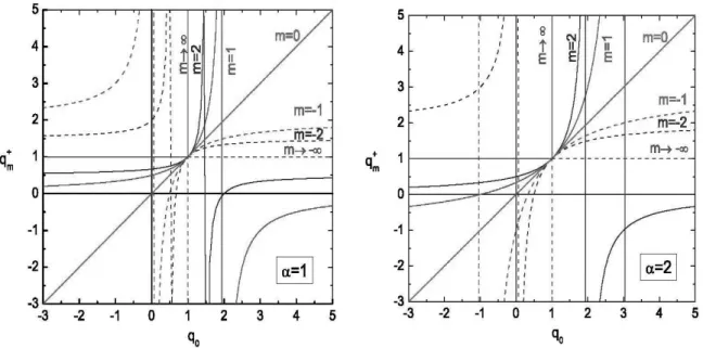
fol-FIG. 6:q+mas a function ofq+0 ≡q0for typical values ofm. For clarity, the vertical asymptotes are indicated as well. Left:α=1;Right:
α=2. For each valuem>0, there are two branches: the left one is such thatq+m>1 (q+m<1) ifq0>1 (q0<1); the right one does not contain the point(q0,q+m) = (1,1). For each valuem<0, there are two branches: the right one is such thatqm+>1 (q+m<1) ifq0>1 (q0<1); the left one does not contain the point(q0,q+m) = (1,1).
FIG. 7:q−mas a function ofq+0 ≡q0for typical values ofm. For clarity, the vertical asymptotes are indicated as well. Left:α=1;Right:
α=2. For each valuem>0, there are two branches: the right one is such thatq+m>1 (q+m<1) ifq0<1 (q0>1); the left one does not contain the point(q0,q+m) = (1,1). For each valuem<0, there are two branches: the left one is such thatqm+>1 (q+m<1) ifq0<1 (q0>1); the right one does not contain the point(q0,q+m) = (1,1).
lowing simple structure. In some caseqmsatisfies
α
1−q+m
= α
1−q0
+m (m=0,±1,±2, ...), (40)
where 0<α≤2. In other cases it satisfies, through the
so-calledadditive duality q0↔(2−q0),
α
1−q−m
= α
q0−1
+m (m=0,±1,±2, ...), (41)
words, for fixed(α,m), we have that
q−m(q−m(q0)) =q0,∀q0. (42) Or equivalently, the functionq−m(q0)concides with the func-tionq0(q−m).
It respectively follows from (40) and (41) that
α
1−q+m−
m= α
1−q+m′ −m
′ (m,m′=0,±1,±2, ...), (43)
and
α
1−q−m−
m= α
1−q−m′ −m
′ (m,m′=0,±1,±2, ...). (44)
If we defineq+m(q0)through Eq. (40) andq−m(q0)through Eq. (41), we easily see that
q−m(q0) =q+m(2−q0). (45) If we make an analytical extension in (40) such thatmand m′are allowed to be real numbers, we may consider the case
m′=m−α (0<α≤2). (46) By replacing this into Eqs. (43) and (44), we respectively obtain
q+m−α=2− 1 q+m
, (47)
and
q−m−α=2− 1 q−m
. (48)
This specific form of connection appears in very many occa-sions in nonextensive statistical mechanics. In particular, if
α=1 we have
q+m−1=2− 1 q+m
, (49)
and
q−m−1=2− 1 q−m
. (50)
And ifα=2 we have
q+m−2=2− 1 q+m
. (51)
and
q−m−2=2− 1 q−m
. (52)
The families (40) and (41) can be respectively rewritten as follows:
q+m=αq0+ (1−q0)m α+ (1−q0)m
(m=0,±1,±2, ...), (53) and
q−m=α(2−q0) + (q0−1)m α+ (q0−1)m
(m=0,±1,±2, ...). (54)
In both cases we verify thatq0=1 yieldsqm=1, ∀m, and thatq±±∞=1, ∀q06=1. For one of the two branches of the family (53) we verify thatq0>1 impliesq+m>1,∀m, and that
q0<1 impliesq+m<1, ∀m. For one of the two branches of the family (54) it is the other way around, i.e,q0>1 implies q−m <1,∀m, andq0<1 implies q−m>1, ∀m. It is possible to simultaneously write both families in a compact manner, namely
q±m=α[1±(q0−1)]±(1−q0)m α±(1−q0)m
(m=0,±1,±2, ...). (55) These relations exhibit a vertical asymptote at q0=1±mα, and a horizontal asymptote atq±m=1∓αm.
It is also worth stressing two interesting properties ofq−m. First, we verify that
q−0 =2−q0, (56)
which precisely recovers the already mentionedadditive du-ality. This duality admits only one fixed point, namelyq0=1.
Second, we verify that
lim m→αq
− m=
1
q0, (57)
which precisely is the so-calledmultiplicative duality. This duality admits two fixed points, namelyq0=1 andq0=−1. It can be shown [10, 58] that, by successively and alterna-tively composing these two dualities, the entire basic structure of Eqs. (55) can be recovered. To the best of our knowledge, the family (55), as a set of transformations, first appeared in [73], and, since then, in an amazing amount of other situ-ations. Moreover, isolated elements of the family (55) had been present in the literature even before the paper [73]. The exhaustive list of these many situations is out of the present scope. Let us, however, mention a few paradigmatic ones.
First, theq-Fourier transform (that we will discuss in Sec-tion 4), when applied to(q,α)-stable distributions, involves [20, 74, 75] the transformation (53).
Second, theq-Fourier transform forq<1 can be obtained from that corresponding toq>1 by using the transformation [76]
2 q−1−1 =
2 1−q0
+1, (58)
which transforms the interval[1,3)into the interval(−∞,1]
(see Fig. 5 ). This transformation is precisely the(α,m) = (2,−1)element of family (54).
Third, elements of these families appear in what is some-times called theq-triplet, which we address specifically in the next Subsection.
The sets (53) and (54) are illustrated in Figs. 6 and 7 re-spectively.
3.4. Theq-triplet
This set is currently referred to as theq-triangle, or the q-triplet. In theBGlimit, it should beqsensitivity=qrelaxation=
qsensitivity=1.
One year later, theq-triplet was indeed found in the solar wind [78] through the analysis of the magnetic-field data sent to Earth (NASA Goddard Space Flight Center) by the space-craft Voyager 1, at the time in the distant heliosphere. The observations led to the following values:
qsensitivity = −0.6±0.2, (59)
qrelaxation = 3.8±0.3, (60)
qstationary state = 1.75±0.06. (61) The most preciseqbeingqstationary state, it seems reasonable to fix it at its nominal value, i.e.,
qstationary state=7/4. (62) By heuristically adopting simple relations belonging to the set (53), we can conjecture [58]
qrelaxation=2− 1 qsensitivity
, (63)
and
qstationary state=2− 1 qrelaxation
. (64)
Eqs. (62), (63) and (64) lead to
qsensitivity = −1/2, (65)
qrelaxation = 4, (66)
qstationary state = 7/4, (67) which, within the error bars, are consistent with the observed values (59), (60) and (61). These assumptions are consistent with the following identification:
qsensitivity ≡ q+m, (68)
qrelaxation ≡ q+m−α, (69)
qstationary state ≡ q+m−2α. (70)
They are also consistent with the following identification
qsensitivity ≡ q−m, (71)
qrelaxation ≡ q−m−α, (72)
qstationary state ≡ q−m−2α. (73)
Although this kind of scenario is tempting, we have not yet achieved a deep understanding which would provide a phys-ical justification about it. To make things even more intrigu-ing, a last remarkable discovery [10, 79] deserves mention. Through the definitionε≡1−q, we have
εsensitivity ≡ 1−qsensitivity=1−(−1/2) =3/2, (74) εrelaxation ≡ 1−qrelaxation=1−4=−3, (75) εstationary state ≡ 1−qstationary state=1−7/4=−3/4(76). Amazingly enough, these values satisfy
εstationary state =
εsensitivity+εrelaxation
2 , (77)
εsensitivity = √εstationary stateεrelaxation, (78)
ε−relaxation1 = ε
−1
sensitivity+ε−stationary state1
2 , . (79)
which are the arithmetic, geometric and harmonic means re-spectively! All these striking features suggest something like a deep symmetry, which eludes us. In any case, even if notori-ously incomplete, the whole story was apparently considered quite stimulating by the organizers of the United Nations In-ternational Heliophysical Year 2007. Indeed, they prepared the poster shown in Fig. 8 for the exhibition organized during the launching of the IHY in Vienna.
One more interestingq-triplet is presently known, namely for the edge of chaos of the logistic map. It is given by
qsensitivity = 0.244487701341282066198... , (80)
qrelaxation = 2.249784109... , (81)
qstationary state = 1.65±0.05. (82) We remind that, for this case, qentropy production =qsensitivity. See [80–83] for the value (81), and [84, 85] for the value (82). No simple relations seem to hold between these three num-bers. We notice, however, that, for bothq-triplets that have been presented in this Subsection, the following inequalities hold:
qsensitivity≤1≤qstationary state≤qrelaxation. (83)
4. q-GENERALIZING THE CENTRAL LIMIT THEOREM, OR WHY ARE THERE SO MANYq-GAUSSIAN-LIKE
DISTRIBUTIONS IN NATURE?
4.1. Central limit theorems andq-Fourier transforms
The Central Limit Theorem (CLT) with its Gaussian attrac-tors (in the space of probability distributions) constitutes one of the main pieces mathematically grounding important parts ofBGstatistical mechanics.
For instance, if we extremizeSBG=−k
R∞
−∞dx p(x)lnp(x)
with the constraintsR∞
−∞dx p(x) =1,hxi ≡
R∞
−∞dx x p(x) =0
andhx2i ≡R∞
−∞dx x2p(x) =σ2, we straightforwardly obtain
the following equilibrium distribution:
pBG(x) =
e−βx2
R∞
−∞dx e−βx
2, (84)
i.e., a Gaussian, where the Lagrange parameterβ>0 is de-termined through theσ2-constraint.
On a different vein — still within the realm ofBGstatistical mechanics —, the most basic free-particle Langevin equation (with additive noise), and its associated Fokker-Planck equa-tion, provide, for all times and positions, a Gaussian distribu-tion.
As a third connection, one might argue that the velocity dis-tribution ofanyparticle of a system described by a classical N-particle Hamiltonian with kinetic energy and (short-range) two-body interactions is the Maxwellian distribution, i.e., a Gaussian. Now, thiscomes outfromBGstatistics. So, in what sense may we consider that theCLTenters? In the sense that Maxwellian distributions are indeed ubiquitously observed in nature, and this happens because, for not too strong perturba-tions, Gaussians areattractors.
FIG. 8: Poster prepared by the organizers of the Opening Ceremony of the International Heliophysical Year 2007 for its accompanying exhibition, the 27 February 2007 in Vienna.
and references therein for the reasons which enabled conjec-turing thisq-generalization).
We do not intend in the present review to be exhaustive with regard to this rich subject. Let us nevertheless remind that the extremization ofSqunder essentially the same con-straints as before (i.e., normalization, symmetry, and finite-ness of the width of the distribution) yields, as the stationary-state distribution, the followingq-Gaussian:
pq(x) =
e−qβx2
R∞
−∞dx e− βx2
q
(q<3;β>0). (85)
Let us now briefly review the standardCLT as well as the occasionally called L´evy-Gnedenko theorem. If we have N equal independent(or quasi-independent in an appropri-ate manner) random variables xi (i=1,2, ...,N), their sum
XN≡∑Ni=1xiconverges (after appropriate centering and scal-ing withN) onto a Gaussian distribution in theN→∞limit if the variance of the elementary distribution isfinite. Such is the case, for instance, forq-Gaussians withq<5/3. If the variance of the elementary distributiondiverges(and the dis-tribution asymptotically decays like a power-law), the sumXN converges, instead, onto anα-stable L´evy distribution. Such
is the case, for instance, forq-Gaussians with 5/3<q<3. In this case, through the|x| →∞asymptotics, the L´evy indexα
is related to the indexqthrough
α=3−q
q−1 (5/3<q<3). (86) The situation changes drastically if the hypothesis of (quasi-)independence is violated, i.e., if theN variables are strongly correlated. In this case, one expects the attractor to be neither Gaussian norα-stable. If this correlation is of the type denoted asq-independence(1-independence being independence) [20], then the attractor of the sumXN is aq -Gaussian if a specificq-generalized variance isfinite, and a
(q,α)-stable distribution if itdiverges. These are the respec-tive q-generalizations of Gaussians and L´evy distributions. See Fig. 9.
The proof of theseq-generalizedCLTtheorems is based on the so calledq-Fourier transform, defined as follows [20, 74, 75, 88, 89]:
Fq[f](ξ)≡
Z
dx eixqξ⊗qf(x) =
Z
FIG. 9:N1/[α)2−q)]-scaled attractors F(x) when summingN→∞q-independent identical random variables with symmetric distribution f(x)
withQ-varianceσQ≡R−∞∞dx x2[f(x)]Q/
R∞
−∞dx[f(x)]Q(Q≡2q−1;q1= (1+q)/(3−q);q≥1). Top left:The attractor is the Gaussian sharing withf(x)the same varianceσ1(standard CLT).Bottom left:The attractor is theα-stable L´evy distribution which shares withf(x)the same asymptotic behavior, i.e., the coefficientCα(L´evy-Gnedenko CLT, orα-generalization of the standard CLT).Top right:The attractor is theq-Gaussian which shares with f(x)the same(2q−1)-variance, i.e., the coefficientCq(q-generalization of the standard CLT, orq-CLT).
Bottom right: The attractor is the(q,α)-stable distribution which shares with f(x)the same asymptotic behavior, i.e., the coefficientCqL,α (q-generalization of the L´evy-Gnedenko CLT andα-generalization of theq-CLT). The caseα<2, for bothq=1 andq6=1 (more precisely
q>1), further demands specific asymptotics for the attractors to be those indicated; essentially the divergentq-variance must be due to fat tails of the power-law class, except for possible logarithmic corrections (for theq=1 case see, for instance, [87] and references therein).
transformation (58) [76]. Theq-Fourier transform (which is nonlinearifq6=1) has a remarkable property, namely to be closed within the family ofq-Gaussians. More precisely, the q-Fourier transform of a (normalized)q-Gaussian, as given by Eq. (85), is another member of theq-Gaussian family, namely one having its index given by
q1= 1+q
3−q, (88)
which admits q=1 as a fixed point (corresponding to the standard Fourier tranform). It can be rewritten as follows:
2 1−q1
= 2
1−q+1, (89)
which, through Eq. (40), immediately allows for the identifi-cation(q,q1)≡(q0,q+1)forα=2.
This transformation, together with the corresponding one forβ, is straightforwardly reversible. However, for a density f(x)notbelonging to the family ofq-Gaussians, the problem can be more complex. Hilhorst has introduced [90] two inter-esting and paradigmatic examples which illustrate the diffi-culty. One of them is presented in his article [91] in this same volume. We shall here discuss his other example, which we present in what follows. Let us define the probability density
f(x,a)≡
√ 2
π
(1−a|x|)2
[(1−a|x|)2+1 2x2]2
if |x|<1/a
0 otherwise ,
(90)
witha≥0 . We verify that f(x,a)is normalized,∀a, i.e.,
Z 1/a
−1/a
dx f(x,a) =1, ∀a. (91) We also verify that f(x,0)is precisely but a(3/2)-Gaussian, namely
f(x,0) =
√ 2
π
1
(1+1 2x2)2
. (92)
See Fig. 10 for typical examples of f(x,a). Itsq-Fourier transform forq≥1 is given by
Fq[f(x,a)](ξ) =
Z ∞
−∞dx
f(x,a)
{1−(q−1)iξx[f(x,a)]q−1}q−11 .
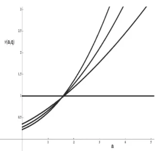
FIG. 10: The distribution f(x,a)for typical values of a: a=2 (blue),a=1 (green), anda=0 (red). From [92].
FIG. 11: Thea-dependence ofµ(a,q)for typical values ofq. From top to bottom on the right side:q=1.6,1.5,1.4,1. From [92].
Replacing herein Eq. (90) we obtain
Fq[f(x,a)](ξ) =
Z 1/a −1/a
dx √
2
π
(1−a|x|)2
[(1−a|x|)2+x2/2]2
n
1−(q−1)iξxh √
2
π
(1−a|x|)2
[(1−a|x|)2+x2/2]2
iq−1oq−11
.(94)
It can be verified thatFq[f(x,a)](ξ)depends onaforany q6= 3/2. But,F3/2[f(x,a)](ξ)doesnotdepend ona. Indeed, it is given by
F3/2[f(x,a)](ξ) = 1
[1+ 1
4π√2ξ
2]3/2, (95)
where we have used the variable changementy= x
1−a|x|. In other words, thisq-Fourier integral transform has, not one, but an entire family of functions (parameterized by the real
FIG. 12: Thea-dependence ofν(a,q)for typical values ofq. From top to bottom on the right side:q=1.6,1.5,1.4,1. From [92].
FIG. 13: Thea-dependence ofhx2i2q−1=µ(a,q)/ν(a,q)for typical values ofq. From top to bottom on the left side:q=1,1.4,1.5,1.6. From [92].
numbera) of pre-images. Hence, unless we add some sup-plementary information,F3/2[f(x,a)](ξ)is not invertible. Let us now discuss this delicate point related to the nonlinearity of the genericq-Fourier transform, a point which evaporates forq=1 since the standard Fourier tranform is a linear one.
We first define the following quantities [23]:
µ2q−1≡
Z 1/a
−1/a
dx x2[f(x,a)]2q−1≡µ(a,q) [µ(0,1) =2], (96) and
ν2q−1≡
Z 1/a −1/a
dx[f(x,a)]2q−1≡ν(a,q) [ν(a,1) =1], (97) which are illustrated in Figs. 11 and 12 respectively. The
(2q−1)-variance is given by
hx2i2q−1≡
R1/a
−1/adx x
2[f(x,a)]2q−1
R1/a
−1/adx[f(x,a)]2q−1
=µ(a,q)
ν(a,q). (98)
This quantity corresponds to the standard (lin-ear) variance, but with the escort distribution
[f(x,a)]2q−1/R1/a
−1/adx′[f(x′,a)]2q−1, instead of the
orig-inalone f(x,a). It is illustrated in Fig. 13.
To fully understand the implications of these results, let us remind that successive moments with appropriate escort dis-tributions are directly related with the successive derivatives of the q-Fourier transform of f(x,a)[23]. Since f(x,a)is an even function, all odd moments, as well as all odd deriva-tives ofFq[f(x,a)](ξ)|ξ=0, vanish. All even such derivatives are finite, in particularµ2q−1∝
d2F
q[f(x,a)](ξ)
dξ2 |ξ=0. We see in Fig. 11 that, for all q6=3/2, µ2q−1monotonicallydepends ona. Therefore, for all such values ofqand within the fam-ily {f(x,a)}, the q-Fourier integral transform is invertible, even being nonlinear. However,notso forq=3/2. Consis-tently,µ(a,3/2)is a constant. In this particular case, further information is needed. This information can be the value of
ν(a,3/2), which, as we verify in Fig. 12,monotonically de-pends ona. In other words, the integral tranformF3/2together with the knowledge of sayν(a,3/2), becomes an invertible operation within the family{f(x,a)}.
An analogy can be done at this point. As we all know, Newton’s equationmd2x(t)
dt2 =F(x)doesnotprovide a single solution but a family of solutions. To have a unique solu-tion we need to provide further informasolu-tion, namelyx(0)and
˙
x(0). An important difference, however, between this prob-lem and the generic invertibility of theq-Fourier transform is that, for the nonlinear integral transform, we donotknow the general form of its inverse. Would we know it, the prob-lem would in principle be completely solvable through the use of supplementary information (such as the value ofnufor the above illustration) which would uniquely determine the specific density within the general form. As we see, the gen-eral problem still remains open. But if we happen to know within which specific family of densities we are working (say q-Gaussians, or say the family{f(x,a)}), uniqueness of the inverse is basically guaranteed.
All the above discussion about invertibility is of course rel-evant for the domain of validity of theq-generalized central limit theorem. At the present moment, its proof [20] fully ap-plies only within the class of densities for which invertibility is guaranteed. This class is very vast; however, as we have seen, it does not include all possible densities. An alternative q-generalizedCLT can be seen in [93].
4.2. Fittings can be extremely useful ... when done carefully!
In this section we compare three analytic forms which are frequently used in the context of complex systems when-ever fat tails emerge. These forms are theq-exponential, the stretched exponential, and the Mittag-Leffler function. All three recover the exponential function as a limiting instance.
Let us remind that theq-exponential functionis defined, for x≥0 andq≥1, as follows:
e−qx≡ 1
[1+ (q−1)x]q−11
(e−1x=e−x), (99)
hence, forβ≥0,
e−qβx≡ 1
[1+ (q−1)βx]q−11
(e−1βx=e−βx) (100)
We immediately verify that
e−qβx∼1−βx (x→0;∀q≥1), (101) and that
e−qβx∼ 1
[(q−1)β]q−11 1
xq−11
∝ 1
xq−11
(x→∞;∀q>1). (102)
Let us finally mention that the function (100) is the solution of
dy dx=−βy
q (103)
withy(0) =1.
Let us consider now, for comparison, thestretched expo-nential function, defined, for 0<α≤1, as follows:
E
α(x)≡esign(x)|x|α
(
E
1(x) =ex), (104) hence, forx≥0 andγ≥0,E
α(−γα1x)≡e−γxα (E
1(−γx) =e−γx) (105) We immediately verify thatE
α(−γ1
αx)∼1−γxα (x→0; 0<α≤1), (106) and that
E
α(−γα1x) =e−γxα (x→∞; 0<α≤1). (107) The function (104) is the solution ofdy
d[sign(x)|x|α] =−γy (108)
withy(0) =1.
Let us now add, within this comparison, theMittag-Leffler functiondefined, for 0<η≤1, as follows (see, for instance, [94–96]):
Eη(x) = ∞
∑
n=0xn
Γ(1+ηn) (E1(x) =e
x).
It follows that, forx≥0 andδ≥0, we have Eη(−(δx)η) =
∞
∑
n=0(−1)n (δx) ηn
Γ(1+ηn), (110)
whose asymptotic behaviors are
Eη(−(δx)η)∼1− (δ
x)η
Γ(1+η) (x→0; 0<η≤1), (111)
and
Eη(−(δx)η)∼ 1
Γ(1−η) (δx)η (x→∞; 0<η<1). (112)
Consequently, this function interpolates between the stretched exponential for small values ofxand the power-law for large values ofx(see Fig. 22 of [95]).
The function (110) satisfies
dηy dxη=−δ
ηy
(113)
withy(0) =1, theCaputo fractional derivative (which dif-fers from theRiemman-Liouville fractional derivative) being defined as follows:
dηy dxη ≡
1
Γ(1−η)
Z x
0 dx′ y
(1)(x′)
(x−x′)η (0<η<1), (114)
wherey(1)(x′)≡dydx(x′′) ;limη→1 dηy dxη =
dy dx.
We see therefore that, if we have access to the x→0 and x→∞ asymptotic behaviors, q-exponentials (q>1), stretched exponentials (0<α<1), and Mittag-Leffler func-tions (0<η<1) are easily distinguishable among them. However, as illustrated in Figs. 14 and 15, their values can be very similar in the intermediate (non asymptotic) region. This fact illustrates a well known concept: careless fittings can be dangerous. They can be however extremely useful if done meticulously. They are, in any case, inescapable when-ever the analysis of experimental or numerical results is con-cerned. Further interesting examples along similar lines can be seen in [91].
The three functions that we have compared here are partic-ular cases of the functiony(x;q,α,η,B)which satisfies
dηy
d(xα)η =−B y q
(115)
with y(0;q,α,η,B) = 1. The q-exponential corresponds to y(x;q,1,1,β); the stretched exponential corresponds to y(x; 1,α,1,γ); and the Mittag-Leffler function corresponds to y(x; 1,1,η,δη). Clearly, at the present time no analytical
ex-pression exists for such a general functiony(x;q,α,η,B).
4.3. q-Gaussian-like distributions in nature and elsewhere
The q-generalized CLT, with itsq-Gaussian attractors in the space of probability densities, applies for correlations of the q-independent type. There is strong evidence that this type of correlations is deeply related to strict or asymptotic
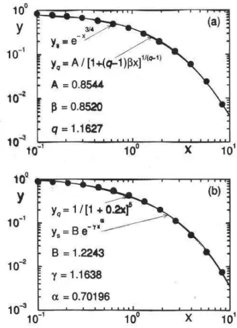
FIG. 14: Comparingq-exponentials with stretched exponentials in log-log scale (which is the most frequent representation of such functions). (a) The dots have been generated with the stretched ex-ponential functiony=e−x3/4, their size has been enlarged in order to mimic experimental error bars, and they have been fitted, within the interval[10−1,10], with theq-exponentialy=A e−βx
q . (b) The dots have been generated with theq-exponential functiony=e−1.x2
, and they have been fitted, within the interval[10−1,10], with the stretched exponentialy=B e−γxα. As we verify in these two typical examples, these fitting functions are numerically indistinguishable within the intermediate interval that we have considered here; only high-precision numerical knowledge of the values of the ”experi-mental“ dots within thex→0 andx→∞asymptotic regions could indicate one or the other, ... or a different one!
scale-invariance (which might well be necessary for q -independence, although surely not sufficient). After decades of studies focusing on fractals, it is by now well established that scale-invariance is ubiquitous in natural, artificial and even social systems. Consequently, we should expect the emergence ofq-Gaussians quite often. This is indeed what happens, as we shall illustrate next (needless to say that only within the error bars corresponding to each case).
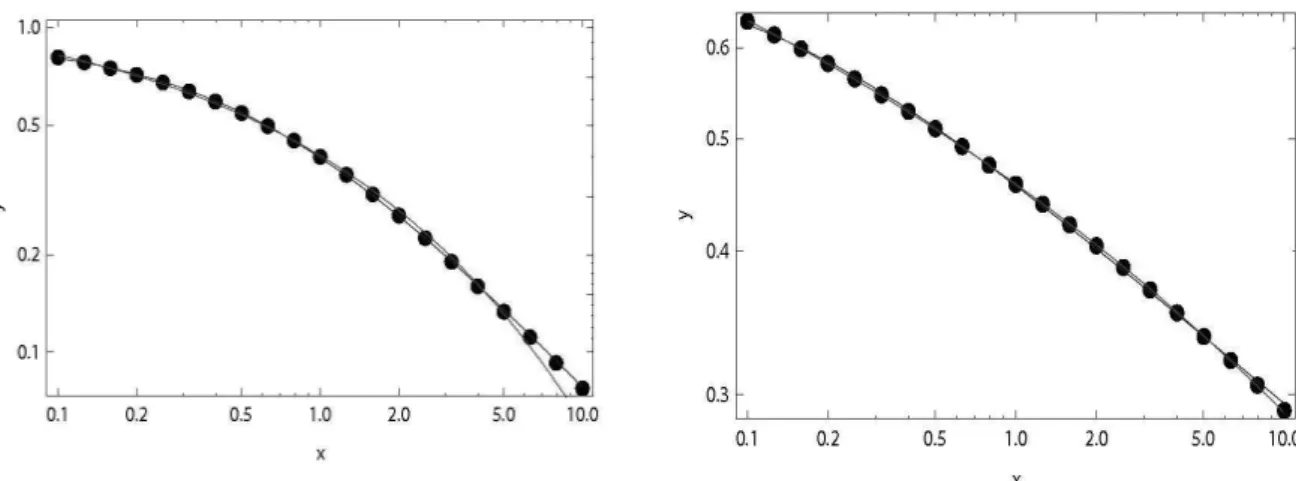
FIG. 15: The dots have been generated with the Mittag-Leffler functiony=Eη(−(δx)η). The upper (lower) curve at the right side is the
q-Gaussiany=A e−qβx(stretched exponentialy=B e−γx
α
) which best fits the present discrete set of 21 values of this Mittag-Leffler func-tion. Left:(η,δ) = (0.7,1),(A,q,β) = (0.915335,2.15899,1.40801)and(B,α,γ) = (1.26496,0.423769,1.14411). Right:(η,δ) = (0.3,1), (A,q,β) = (0.708294,6.06448,1.65478)and(B,α,γ) = (1.45013,0.144472,1.15538). We verify that, within this limited intermediate region and with the precision indicated by the size of the dots, the three functions are nearly indistinguishable. However, the detailed study of their
x→0 andx→∞asymptotic behaviors would allow for discrimination among them.
(ii) The distribution of velocities in quasi-two dimensional dusty plasma has been detected to beq-Gaussian [98, 99].
(iii) Single ions in radio frequency traps interacting with a classical buffer gas (e.g.,136Ba+ion cooled at 300 K) exhibit q-Gaussian distributions [100].
(iv) The distribution of velocities of cells ofHydra viridis-simain solution has been shown to beq-Gaussian [101].
(v) Distribution of velocities of the defects in the so-called defect turbulence have been interpreted asq-Gaussians [102]. (vi) Distributions corresponding to fluctuations of the magnetic field in the plasma within the solar wind in the distant heliosphere and the heliosheath, as detected through data received from the Voyager 1 have been interpreted as q-Gaussians [78, 103–107].
(vii) Computational distributions of velocities in silo drainage of granular matter have been interpreted as q -Gaussians [108, 109].
(viii) Distributions of sums of velocities along the trajec-tories of the particles in a large class of initial conditions leading to the so-called quasi-stationary states of the HMF model (many-body Hamiltonian system describing an in-ertial classical XY ferromagnet with long-range two-body interactions) gradually approach q-Gaussians [110–112]. Let us mention at this point that if, instead of these time averages, we do ensemble averages, we obtain other types of distributions [113, 114].
(ix) Distributions of sums of velocities along the trajec-tories of the particles at the edge of chaos of the Kuramoto model gradually approachq-Gaussians [115].
(x) The distributions of sums of successive iterates in the close neighborhood of the edge of chaos in unimodal dissi-pative maps exhibit slight oscillations (possibly log-periodic) on top ofq-Gaussians [84, 85, 116].
(xi) Return distributions corresponding to earthquakes using data from the World and Southern California catalogs have been interpreted asq-Gaussians [117].
(xii) Return distributions of fluctuations associated with self-organized criticality in the Ehrenfest’s dog-flea model are consistent withq-Gaussians [118].
(xiii) Distributions of the increments of current fluctuations of charge disorder in arrays are interpreted as q-Gaussians [119].
(xiv) Financial return distributions in the New York Stock Exchange, NASDAQ and elsewhere are routinely interpreted asq-Gaussians [120–130].
(xv) Distributions of postural sway for young and old people are interpreted asq-Gaussians [131].
space. Very recently this finally occurred in the experimen-tally observed relaxation curves [132] of paradigmatic spin-glasses such as Cu0.95Mn0.05, Cu0.90Mn0.10, Cu0.84Mn0.16, Cu0.65Mn0.35, andAu0.86Fe0.14.
5. CONCLUSIONS
The magnificent theory of Boltzmann and Gibbs has, as any other intellectual construct, limits of validity. Outside these limits a vast world exists in nature as well as in artificial systems. Some — apparently many — classes of systems of this vast world are adequately addressed by nonextensive statistical mechanics, proposed over twenty years ago [9] as a generalization of the standard theory. The complexity of this extended theory certainly is much higher than that of the BG statistical mechanics. A central feature which dramatically reflects this complexity is the fact that only one value of the index qis to be used for the BG theory, namelyq=1, whereas an entireset of inter-related valuesfor such indices emerges outside it (see, for instance, Figs. 6 and 7). Another feature which also reflects this complexity is the fact that the involved mathematics is definitivelynonlinear, whereas that of the BG theory is, in many aspects, alinear one. Under such circumstances, one could expect to have an extremely slow technical and epistemological progress. The intensive and world-wide developments that we have witnessed during the last two decades neatly show that it has not been so. Indeed, an amazingly large field of knowledge is now
available, demanding for further analytical, experimental, and computational efforts to advance. Sem pressa e sem pausa...(Without hurry and without stops...)
Acknowledgements
The idea of comparing, together with theq-exponential and the stretched exponential functions, the Mittag-Leffler func-tion emerged during an interesting conversafunc-tion with Ryszard Kutner, to whom I am indebted. Along this line, I also thank M.J. Jauregui Rodriguez for the construction of Fig. 15. I thank as well G. Ruiz for the construction of Figs. 6 and 7. I am indebted to H.J. Hilhorst for authorizing me to present his unpublished example, which enables the analysis of the invertibility of theq-Fourier transform out from the family of the q-Gaussians, although within a specific larger fam-ily of densities. I am also indebted to him, as well as to S. Umarov and E.M.F. Curado, for long and fruitful discussions, always on the subject of the nontrivial difficulties related with theq-Fourier transform possible invertibility. My thanks also go to R. Kutner and E.K. Lenzi for useful discussions about fractional derivatives. I am deeply grateful to R.S. Mendes, L.R. Evangelista, L.C. Malacarne and E.K. Lenzi for their ef-ficient organization of, and their delightfully warm hospital-ity at,NEXT2008 - International Conference on Nonextensive Statistical Mechanics: Foundations and Applications, held in Iguassu-Brazil in 27-31 October 2008. Partial financial sup-port by CNPq and FAPERJ (Brazilian agencies) is gratefully acknowledged.
[1] M. Planck,Uber irreversible Strahlugsforgange, Ann d. Phys. (4) (1900) 1, S. 69-122 (see [8]).
[2] M. Planck, Verhandlungen der Deutschen Physikalischen Gessellschaft2, 202 and 237 (1900) (English translation: D. ter Haar, S. G. Brush, Planck’s Original Papers in Quantum Physics (Taylor and Francis, London, 1972)].
[3] L.B. Okun,The fundamental constants of physics, Sov. Phys. Usp.34, 818 (1991).
[4] G. Cohen-Tannoudji,Les Constantes Universelles, Collection
Pluriel(Hachette, Paris, 1998).
[5] C. Tsallis and S. Abe,Advancing Faddeev: Math can deepen Physics understanding, Physics Today51, 114 (1998). [6] L. Okun, Cube or hypercube of natural units?,
hep-th/0112339 (2001).
[7] M.J. Duff, L.B. Okun and G. Veneziano, Trialogue on the number of fundamental constants, JHEP03 (2002) 023 [physics/0110060].
[8] M.J. Duff,Comment on time-variation of fundamental con-stants, hep-th/0208093 (2004).
[9] C. Tsallis,Possible generalization of Boltzmann-Gibbs statis-tics, J. Stat. Phys.52, 479-487 (1988) [The proposal first came to my mind in August 1985, during a scientific event in Mex-ico City, and was further advanced in August 1987, during and immediately after a scientific event in Maceio-Brazil. But it was published only in 1988, particularly stimulated by the fruitful discussions held on the subject with E.M.F. Curado and H.J. Herrmann during the Maceio event].
[10] C. Tsallis,Introduction to Nonextensive Statistical Mechanics - Approaching a Complex World(Springer, New York, 2009). [11] A regularly updated Bibliography can be seen at
http://tsallis.cat.cbpf.br/biblio.htm
[12] C. Tsallis, R.S. Mendes and A.R. Plastino,The role of con-straints within generalized nonextensive statistics, Physica A
261, 534 (1998).
[13] E.M.F. Curado and C. Tsallis,Generalized statistical mechan-ics: connection with thermodynamics, J. Phys. A24, L69 (1991); Corrigenda:24, 3187 (1991) and25, 1019 (1992). [14] S. Abe, Instability of q-averages in nonextensive statistical
mechanics, Europhys. Lett.84, 60006 (2008).
[15] R. Hanel, S. Thurner and C. Tsallis,On the robustness of q-expectation values and R´enyi entropy, Europhysics Letters85, 20005 (2009).
[16] R. Hanel and S. Thurner,Stability criteria for q-expectation values, Phys. Lett. A373, 1415 (2009).
[17] S. Abe and G.B. Bagci,Necessity of q-expectation value in nonextensive statistical mechanics, Phys. Rev. E71, 016139 (2005).
[18] S. Abe,Why q-expectation values must be used in nonexten-sive statistical mechanics, Astrophys. Space Sci.305, 241-245 (2006).
[19] W. Thistleton, J.A. Marsh, K. Nelson and C. Tsallis, Gener-alized Box-Muller method for generating q-Gaussian random deviates, IEEE Transactions on Information Theory53, 4805 (2007).
[20] S. Umarov, C. Tsallis and S. Steinberg,On a q-central limit theorem consistent with nonextensive statistical mechanics, Milan J. Math.76, 307 (2008).
[21] J.-F. Bercher,Tsallis distribution as a standard maximum en-tropy solution with ’tail’ constraint, Phys. Lett. A372, 5657 (2008).
[23] C. Tsallis, A.R. Plastino and R.F. Alvarez-Estrada, Escort mean values and the characterization of power-law-decaying probability densities, J. Math. Phys.50, 043303 (2009). [24] V. Schwammle, F.D. Nobre and E.M.F. Curado,
Conse-quences of the H-theorem from nonlinear Fokker-Planck equations, Phys. Rev. E76, 041123 (2007).
[25] V. Schwammle, E.M.F. Curado and F.D. Nobre, A general nonlinear Fokker-Planck equation and its associated entropy, Eur. Phys. J. B58, 159 (2007).
[26] S. Abe, Generalized molecular chaos hypothesis and H-theorem: Problem of constraints and amendment of nonexten-sive statistical mechanics, Phys. Rev. E79, 041116 (2009). [27] G.L. Ferri, S. Martinez and A. Plastino, The role of
con-straints in Tsallis’ nonextensive treatment revisited, Physica A347, 205 (2005).
[28] S.R.A. Salinas and C. Tsallis, eds., Nonextensive Statisti-cal Mechanics and Thermodynamics, Braz. J. Phys. 29(1) (1999).
[29] S. Abe and Y. Okamoto, eds.,Nonextensive Statistical Me-chanics and Its Applications, SeriesLecture Notes in Physics
(Springer, Berlin, 2001).
[30] P. Grigolini, C. Tsallis and B.J. West, eds., Classical and Quantum Complexity and Nonextensive Thermodynamics, Chaos, Solitons and Fractals13, Issue 3 (2002).
[31] G. Kaniadakis, M. Lissia and A. Rapisarda, eds.,Non Exten-sive Thermodynamics and Physical Applications, Physica A
305, 1/2 (2002).
[32] M. Sugiyama, ed., Nonadditive Entropy and Nonextensive Statistical Mechanics, Continuum Mechanics and Thermody-namics16(Springer-Verlag, Heidelberg, 2004).
[33] H.L. Swinney and C. Tsallis, eds.,Anomalous Distributions, Nonlinear Dynamics and Nonextensivity, Physica D193, Is-sue 1-4 (2004).
[34] M Gell-Mann and C. Tsallis, eds.,Nonextensive Entropy - In-terdisciplinary Applications(Oxford University Press, New York, 2004).
[35] G. Kaniadakis and M. Lissia, eds.,News and Expectations in Thermostatistics, Physica A340, Issue 1-3 (2004).
[36] H.J. Herrmann, M. Barbosa and E.M.F. Curado, eds.,Trends and Perspectives in Extensive and Non-extensive Statistical Mechanics, Physica A344, Issue 3/4 (2004).
[37] C. Beck, G. Benedek, A. Rapisarda and C. Tsallis, eds., Com-plexity, Metastability and Nonextensivity (World Scientific, Singapore, 2005).
[38] J.P. Boon and C. Tsallis, eds.,Nonextensive Statistical Me-chanics: New Trends, New Perspectives, Europhysics News
36, Number 6, 183-231 (EDP Sciences, Paris, 2005). [39] G. Kaniadakis, A. Carbone and M. Lissia, eds.,News,
Expec-tations and Trends in Statistical Physics, Physica A365, Issue 1 (2006).
[40] S. Abe, M. Sakagami and N. Suzuki, eds., Complexity and Nonextensivity - New Trends in Statistical Mechanics, Progress of Theoretical Physics Supplement 162 (Physical Society of Japan, 2006).
[41] S. Abe, H. Herrmann, P. Quarati, A. Rapisarda and C. Tsallis, eds.,Complexity, Metastability and Nonextensivity, American Institute of Physics Conference Proceedings965(New York, 2007).
[42] C. Tsallis, C. Anteneodo, L. Borland and R. Osorio, Nonex-tensive statistical mechanics and economics, Physica A324, 89 (2003).
[43] M. Bologna, C. Tsallis and P. Grigolini, Anomalous diffu-sion associated with nonlinear fractional derivative Fokker-Planck-like equation: Exact time-dependent solutions, Phys. Rev. E62, 2213 (2000).
[44] F.D. Nobre and C. Tsallis,Infiniterange Ising ferromagnet
-Thermodynamic limit within generalized statistical mechan-ics, Physica A213, 337 (1995).
[45] C. Anteneodo and C. Tsallis,Multiplicative noise: A mech-anism leading to nonextensive statistical mechanics, J. Math. Phys.44, 5194 (2003).
[46] F.A. Tamarit, S.A. Cannas and C. Tsallis,Sensitivity to initial conditions in the Bak-Sneppen model of biological evolution, Eur. Phys. J. B1, 545 (1998).
[47] C. Anteneodo and C. Tsallis,Two-dimensional turbulence in pure-electron plasma: A nonextensive thermostatistical de-scription, J. Mol. Liq.71, 255 (1997).
[48] L. Nivanen, A. Le Mehaute and Q.A. Wang,Generalized al-gebra within a nonextensive statistics, Rep. Math. Phys.52, 437 (2003).
[49] E.P. Borges,A possible deformed algebra and calculus in-spired in nonextensive thermostatistics, Physica A340, 95 (2004).
[50] A.R. Plastino and A. Plastino,Non-extensive statistical me-chanics and generalized Fokker-Planck equation, Physica A
222, 347 (1995).
[51] C. Tsallis and D.J. Bukman,Anomalous diffusion in the pres-ence of external forces: exact time-dependent solutions and their thermostatistical basis, Phys. Rev. E54, R2197 (1996). [52] M.A. Fuentes and M.O. Caceres,Computing the non-linear
anomalous diffusion equation from first principles, Phys. Lett. A372, 1236 (2008).
[53] L. Borland,Ito-Langevin equations within generalized ther-mostatistics, Phys. Lett. A245, 67 (1998).
[54] A.M. Mariz and C. Tsallis, (2009) in progress.


![FIG. 4: S Q for various values of Q for the probabilistic model with N correlated binary variables in [60], corresponding to q limit = 1.5.](https://thumb-eu.123doks.com/thumbv2/123dok_br/18983146.457813/7.892.486.786.77.398/various-values-probabilistic-model-correlated-binary-variables-corresponding.webp)