Nonextensive Statistics:
Theoretical, Experimental and Computational
Evidences and Connections
Constantino Tsallis Centro Brasileiro de Pesquisas Fsicas
Rua Xavier Sigaud 150, 22290-180 Rio de Janeiro-RJ, Brazil e-mail: [email protected]
Received 07 December, 1998
The domain of validity of standard thermodynamics and Boltzmann-Gibbs statistical me-chanics is discussed and then formally enlarged in order to hopefully cover a variety of anomalous systems. The generalization concerns nonextensive systems, where nonextensiv-ity is understood in the thermodynamical sense. This generalization was rst proposed in 1988 inspired by the probabilistic description of multifractal geometries, and has been in-tensively studied during this decade. In the present eort, after introducing some historical background, we briey describe the formalism, and then exhibit the present status in what concerns theoretical, experimental and computational evidences and connections, as well as some perspectives for the future. In addition to these, here and there we point out various (possibly) relevant questions, whose answer would certainly clarify our current understand-ing of the foundations of statistical mechanics and its thermodynamical implications.
I Introduction
A diuse belief exists, among many physicists as well as other scientists, that Boltzmann-Gibbs (BG) statistical mechanics and standard thermodynamics are eternal and universal. It is certainly fair to say that \eter-nal", in precisely the same sense that Newtonian me-chanics is \eternal", they indeed are. But, again in complete analogy with Newtonian mechanics, we can by no means consider them as universal. Indeed, we all know that, when the involved velocities approach that of light, Newtonian mechanics becomes only an approximation (an increasingly bad one) and reality is better described by special relativity. Analogously, when the involved masses are as small as say the elec-tron mass, once again Newtonian mechanics becomes but a (bad) approximation,and quantum mechanics be-comes necessary to understand nature. Also, if the in-volved masses are very large, Newtonian mechanics has to be extended into general relativity. In these senses we certainly cannot consider Newtonian mechanics as
case, some kind of extension appears to become nec-essary. Indeed, an everyday increasing list of physical anomalies are, here and there, being pointed out which defy (not to say that plainly violates) the standard BG prescriptions. A nonextensive thermostatistics, which recovers the extensive, BG one as particular case, was proposed in 1988 [1, 2] which might correctly cover at least some of the known anomalies. Although a fair amount of what legitimately looks like being successful applications is nowadays accumulating, further verica-tions and deeper understanding is needed and welcome. Computational work is highly desired since, on various grounds, the analytic discussion frankly appears to be untractable. Needless, of course, to say that more ex-perimental and theoretical work is absolutely relevant to exhibit the applicability and robustness of the ideas I intend to present herein. In the present contribution, I propose some (hopefully relevant) questions that are right now open to such theoretical, experimental and computational contributions.
Let us be more specic. As mentioned above, it is nowadays quite well known that a variety of physical systems exist for which the powerful (and beautiful) BG statistical mechanics and standard ther-modynamics present serious diculties or anomalies, which can occasionally achieve the status of just plain failures. Within a long list that will be sys-tematically focused on later on, we may mention at this point systems involving long-range interactions (e.g., d = 3 gravitation)[3], long-range microscopic memory (e.g., nonmarkovian stochastic processes, on which much remains to be known, in fact)[4, 5], and, generally speaking, conservative (e.g., Hamilto-nian) or dissipative systems which in one way or an-other involve a relevant space-time (hence, a relevant phase space) which has a (multi)fractal-like structure. For instance, pure-electron plasma two-dimensional turbulence[6], Levy anomalous diusion[7], granular systems[8], phonon-electron anomalous thermalization in ion-bombarded solids ([9] and references therein), so-lar neutrinos[10], peculiar velocities of galaxies[11], in-verse bremsstrahlung in plasma[12] and black holes[13], to cite a few, clearly appear to be (in some cases), or could possibly be (in others), concrete examples. The
present status of these and others will be discussed in Sections III, IV and V.
II Formalism
I I.1 Entropy
As an attempt to overcome at least some of these diculties a proposal has been advanced, one decade ago[1], (see also [14, 15]), which is based on a general-ized entropic form, namely
S q=
k 1,
P W i=1
p q i q,1
W X i=1 p
i= 1; q2R
! ; (1) wherekis a positive constant andW is the total num-ber of microscopic possibilities of the system (for the q < 0 case, care must be taken to exclude all those possibilities whose probability is not strictly positive, otherwise S
q would diverge; such care is not necessary forq>0; due to this property, the entropy is said to be
expansibleforq>0). This expression recovers the usual BG entropy (,k
P W i=1
p i ln
p
i) in the limit
q!1. The entropic indexq(intimately related to and determined by the microscopic dynamics, as we shall mention later on) characterizes the degree of nonextensivityreected in the followingpseudo-additivityentropy rule
S q(
A+B)=k = [S q(
A)=k] + [S q(
B)=k] + (1,q)[S
q( A)=k][S
q(
B)=k]; (2) whereAandBare twoindependentsystems in the sense that the probabilities of A+B factorizeinto those of A and of B (i.e.,p
ij(
A+B) = p i(
A)p j(
B)). We im-mediately see that, since in all cases S
q
0 (
nonneg-ativity property), q < 1; q = 1 and q > 1 respec-tively correspond to superadditivity (superextensivity), additivity (extensivity) and subadditivity (subextensiv-ity). Eq. (2) exhibits a property which has appar-ently never been focused before, and which we shall from now on refer to as the composabilityproperty. It concerns the nontrivial fact that the entropyS(A+B) of a system composed of two independent subsystems A and B can be calculated from the entropies S(A) and S(B) of the subsystems, without any need of
mi-croscopic knowledge about A and B, other than the
nonextensive universality class, represented by the en-tropic index q, i.e., without any knowledge about the microscopic possibilities of A and B nor their associ-ated probabilities. This property is so obvious for the BG entropic form that the (false) idea thatallentropic forms automatically satisfy it could easily install itself in the mind of most physicists. To show
counterexam-ples, it is enough to check that the recently introduced Anteneodo-Plastino[16] and Curado[17] entropic forms satisfy a variety of interesting properties, and neverthe-less are not composable.
The above pseudo-extensivity property can be equivalently written as follows:
c ln[1 + (1,q)Sq(A+B)=k]
1,q
= ln[1 + (1,q)Sq(A)=k] 1,q
+ ln[1 + (1,q)Sq(B)=k] 1,q
(3)
d We come back onto this form later on in connection with Renyi's entropy.
Another important (since it eloquently exhibits the surprising eects of nonextensivity) property is the fol-lowing. Suppose that the set ofW possibilities is
arbi-trarily separated into two subsets having respectively WL and WM possibilities (WL +WM = W). We dene pL
PW L
i=1
pi and pM PW
i=WL+1
pi, hence pL+pM = 1. It can then be straightforwardly estab-lished that
c
Sq(fpig) = Sq(pL;pM) +pqLSq(fpi=pLg) + pqMSq(fpi=pMg); (4) d
where the setsfpi=pLgandfpi=pMgare theconditional probabilities. This would precisely be the famous Shan-non property were it not for the fact that, in front of the entropies associated with the conditional probabil-ities, there appear pqL and pqM instead of pL and pM . This fact will play, as we shall see later on, a central role in the whole generalization of thermostatistics. Indeed, since the probabilitiesfpigare generically numbers be-tween zero and unity, pqi > pi for q < 1 and pqi < pi forq>1, henceq<1 andq>1 will respectively priv-ilegiate the rare and the frequent events. This simple property lies at the heart of the whole proposal. Santos has recently shown[18], strictly following along the lines of Shannon himself, that, if we assume (i) continuity (in thefpig) of the entropy, (ii) increasing monotonicity of the entropy as a function ofW in the case of equiproba-bility, (iii) property (2), and (iv) property (4), thenonly one entropic form exists, namely that given in
deni-tion(1). Of course, the generalization of Eq. (4) to the case where, instead of two, we have Rnonintersecting subsets (W
1+ W
2+
:::+WR=W) is straightforward[19]. To be more specic, if we dene
j X
Wjterms
pi (j= 1;2;:::;R) (5) (hencePR
j=1
j = 1), Eq. (4) is generalized into Sq(fpig) =Sq(fjg) +
R
X
j=1
qjSq(fpi=jg) (6) where we notice, in the last term, the emergence of what we shall soon introduce generically as the unnormal-ized q-expectation value (of the conditional entropies Sq(fpi=jg), in the present case).
Another interesting property is the following. The Boltzmann-Gibbs entropyS
1satises the relation ,k
" d d
W
X
i=1 pi
#
=1 =,k
W
X
i=1
pi ln pi S 1
Moreover, Jackson introduced in 1909[20] the general-ized dierential operator (applied to an arbitrary func-tion f(x))
Dq f(x)
f(qx),f(x) qx,x ;
(8) which satises D1
lim
q !1Dq = d
dx. Abe[21] recently remarked that ,k " Dq W X i=1 p i # =1
= k1, P
W i=1p
q i q,1
S
q (9)
This property provides some insight into the generalized entropic form Sq . Indeed, the inspiration for its use in order to generalize the usual thermal statistics came[1] from multifractals, and its applications concern, in one way or another, systems which exhibit scale invariance. Therefore, its connection with Jackson's dierential op-erator appears to be rather natural. Indeed, this oper-ator \tests" the function f(x) underdilatationof x, in contrast to the usual derivative, which \tests" it under translationof x.
Another property which no doubt must be men-tioned in the present introduction is that Sq is consis-tent with Laplace's maximum ignorance principle, i.e., it is extremum atequiprobability(pi= 1=W
8i). This extremum is given by
Sq = kW 1,q
,1 1,q
(W 1) (10)
which, in the limit q!1, reproduces Boltzmann's cel-ebrated formula S = kln W (carved on his marble grave in the Central Cemetery of Vienna). In the limit W !1, S
qdiverges if q
1, and saturates at k=(q,1) if q > 1.
Finally, let us close the present set of properties by reminding that Sq has, with regard to
fp i
g, a
def-inite concavity for all values of q (Sq is always con-cave for q > 0 and always convex for q < 0). In this sense, it contrasts with Renyi's entropy SR
q (ln P W i=1p q i)=(1
,q) =fln [1 + (1,q)S q=k]
g=(1,q), which does not have this property forallvalues of q .
Before addressing other relevant quantities, let us introduce the following convenient functions[22]:
ex q
[1 + (1,q) x] 1=(1,q );
8(x;q) (11) (hence, ex
1 = e
x) with the denition supplement, for q < 1, that ex
q = 0 if 1 + (1
,q) x 0, (and analo-gously, for q > 1, ex
q diverges at x = 1=(q
,1)) and lnq x
[x 1,q
,1]=[1,q]; 8(x;q) (12)
(hence, ln1 x = ln x). We can easily verify that eln
q x q = ln
q e x q = x;
8(x;q): (13) For instance, Eq. (10) can be rewritten in the following Boltzmann-like form:
Sq = k lnq W (14)
Let us also introduce the following unnormalized q -expectation value:
hAi q W X i=1 pq i A i (15)
hence hAi
1 corresponds to the standard mean value of a physical quantity A.
If our system is a generic quantum one, its proba-bilistic description is given by the density operator , whose eigenvalues are the fp
i
g. Then, the generalized entropy is given by
Sq = k 1 ,Tr
q q,1
(Tr = 1) (16)
and the unnormalized q-expectation value of an observ-able A which does not necessarily commute with is given by
hAi q
Tr
qA : (17)
Eq. (16) can be rewritten as Sq =
,khln q
i
q ; (18)
and also as
Sq = ,khln
2,q i
1 : (19)
If our system is a generic classical one, the rele-vant variables are typically continuous variables, and its probabilistic description is given by a distribution of probabilities p(r), where r is a dimensionless variable in a many-body phase space. Then, the generalized entropy is given by
Sq = k 1 ,
R
dr[p(r)] q q,1
(Z
drp(r) = 1) (20) and the unnormalized q-expectation value of an observ-able A(r) is given by
hAi q
Z
dr[p(r)] qA(
Although we shall, in what follows, be illustrating the present formalism with the case of W discrete micro-scopic possibilities, the generic quantum and classical discussions follow along the same lines,mutatis mutan-dis.
II.2 Canonical ensemble
Once we have a generalized entropic form, as given in Eq. (1) (or an even more general one, or a dierent one), we can use it in a variety of ways. For instance, if we are interested in information theory, some opti-mization algorithms, image processing, among others, we can take advantage of a particular form in dierent ways. See, for instance, [17, 19, 23, 24] and references therein, where it can be veried that not less than 25 (!) dierent entropic forms have received, along the years, a great variety of technological and mathematical ap-plications. For instance, the Renyi entropy mentioned above has been quite useful in the geometrical charac-terization of strange attractors and similar multifractal structures (see [25] and references therein).
However, if our primary interest is Physics, this is to say the (qualitative and quantitative) description and possible understanding of phenomena occurring in Na-ture, then we are naturally led to use the available gen-eralized entropy in order to generalize statistical me-chanics itself and, if unavoidable, even thermodynam-ics. It is along this line that we shall proceed from now on (see also [26]). To do so, the rst nontrivial (and quite ubiquitous) physical situation is that in which a given system is in contact with a thermostat at tem-perature T. To study this, we shall follow along Gibbs' path and focus the so calledcanonical ensemble. More precisely, to obtain the thermal equilibriumdistribution associated with a conservative (Hamiltonian) physical system in contact with the thermostat we shall extrem-ize Squnder appropriate constraints. These constraints are[15]
W X i=1
pi= 1 (norm constraint) (22)
and
hh i
ii q
P
W i=1p
q i
i P
W i=1p
q i
= Uq (energy constraint) (23) where f
i
g are the eigenvalues of the Hamiltonian of the system. We shall refer to hh:::ii
q as thenormalized
q-expectation valueand to Uq as thegeneralized
inter-nal energy (assumednite and xed). It is clear that, in the q ! 1 limit, these quantities recover the stan-dard mean value and internal energy respectively. We immediately verify that, for any observable,
hh:::ii q=
h:::i q h1i
q
(24)
The outcome of this optimization procedure is given by
pi = h
1,(1,q)( i
,U q)=
P W j=1(p
j) q
i 1 1,q Zq
(25) with
Zq()
W X i=1 2 41
,(1,q)( i
,U q)=
W X j=1
(pj) q
3 5
1 1,q (26) It can be shown that, for the case q < 1, the expression of the equilibrium distribution is supplemented by the auxiliary condition that pi= 0 whenever the argument of the function becomes negative (cut-o condition). Also, it can be shown[15] that
1=T = @Sq=@Uq;
8q (T 1=(k)): (27) Furthermore, it is important to notice that, if we add a constant 0 to all
f i
g, we have (as it can be self-consistently proved) that Uq becomes Uq + 0, which leaves invariant the dierencesf
i ,U
q
g, which, in turn, (self-consistently) leavesinvariant the set of probabili-tiesfp
i
g, hence allthe thermostatistical quantities. It is also trivial to show that, for the independent sys-tems A and B mentioned previously, Uq(A + B) = Uq(A) + Uq(B), thus recovering the same form of the standard (q = 1) thermodynamics.
It can be shown that the following relations hold:
W X i=1
(pi) q = ( Z
q)
1,q; (28)
Fq U
q ,TS
q = ,
1 (Zq)
1,q ,1 1,q
and U q = , @ @ (Z q) 1,q ,1 1,q
; (30) where (Z q) 1,q ,1 1,q
= ( Z q)
1,q ,1 1,q
,U
q
: (31)
Let us now make an important remark. If we take out as factors, in both numerator and denominator of Eq. (25), the quantity h
1 + (1,q)U q = P W j=1( p j) q i , and then cancel them, we obtain
c
p i(
) = [1
,(1,q) 0 i] 1 1,q Z 0 q 0 @ Z 0 q W X j=1
[1,(1,q) 0 j] 1 1,q 1 A (32) d with 0= P W j=1( p j) q
+ (1,q)U q
(T 0
1=(k 0))
(33) where
0 is an increasing function of [27].
Let us now address the all important question of the connection between experimental numbers (those pro-vided by measurements), and the quantities that ap-pear in the theory. The denition of U
q suggests the followingnormalizedq-expectation values
O q hhO i ii q P W i=1 p q i O i P W i=1 p q i (34) where O is any observable which commutes with the Hamiltonian, hence with . If it does not commute, Eq. (34) is generalized into
O q Tr q O Tr q (35) Consistently,O
q is the mathematical object to be iden-tied with the numerical value provided by the exper-imental measure. Later on, we come back onto this crucial point.
At this point let us make some observations about the set ofescort probabilities[28]fP
(q ) i
gdened through P (q ) i p q i P W j=1 p q j (W X i=1 P (q )
i = 1) (36)
from which follows the dual relation
p i= [
P (q ) i ] 1 q P W j=1[ P (q ) j ] 1 q : (37)
TheW = 2 illustration of P (q )
i is shown in Fig. 1. As anticipated,q<1 (q>1) privileges therare(frequent) events.
Figure 1. W = 2 illustratio n of the escort probabiliti es: P (q ) = p q p q +(1,p) q .
Let us rst comment that Eqs. (36) and (37) have, within the present formalism, a role somehow analo-gous to the direct and inverse Lorentz transformations in Special Relativity (see [29] and references therein). Second, we notice thatO
q becomes a usual mean value when expressed in terms of the probabilitiesfP
(q ) i
The nal equilibrium distribution reads P(q )
i = [1
,(1,q) 0
i] q 1,q P
W k =1[1
,(1,q) 0
k] q 1,q
: (40)
If the energy spectrum f i
g is associated with the set of degeneracies fg
i
g, then the above probability leads to (associated with the leveli and not thestatei)
P(i) =
gi[1
,(1,q) 0
i] q 1,q P
alllev elsg k[1
,(1,q) 0
k] q 1,q
: (41)
If the energy spectrum f i
gis so dense that can prac-tically be considered as a continuum, then the discrete degeneracies yield the function density of states g(), hence
P() = g() [1,(1,q) 0]
q 1,q R
d0g(0)[1
,(1,q) 00]
q 1,q
(42) The density of states is of course to be calculated for every specic Hamiltonian (given the boundary con-ditions). For instance, for a d-dimensional ideal gas of particles or quasiparticles, it is given[30] by g() / d
,1, where is the exponent characterizing the en-ergy spectrum /K
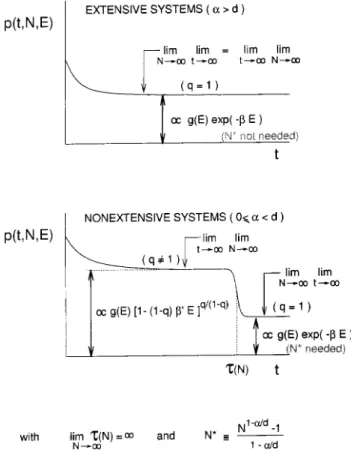
where K is the wavevector (e.g., = 1 corresponds to the harmonic oscillator, = 2 corresponds to a nonrelativistic particle in an innitely high square well, etc). In Figs. 2 and 3 we see typical energy distributions for the particular case of a constant density of states. Of course, the q = 1 case reproduces the celebrated Boltzmann factor. Notice the cut-o for q < 1 and the long algebraic tail for q > 1.
All the above considerations refer, strictly speak-ing, to thermodynamic equilibrium. The word thermo-dynamicmakes allusion to \very large" (N!1, where N is the number of microscopic particles of the phys-ical system). The word equilibrium makes allusion to asymptotically large times (t ! 1 limit) (assuming a stationary state is eventually achieved). The ques-tion arises: which of them rst? Indeed, although both possibilities clearly deserve the denomination \thermo-dynamic equilibrium", nonuniform convergences might be involved in such a way that limN!1limt!1 could dier from limt!1 limN!1. To illustrate this sit-uation, let us imagine a classical Hamiltonian system including two-body interactions decaying at long dis-tances as 1=ron a d-dimensional space, with
0. If > d the interactions are essentially short-ranged, the
two limits just mentioned are basically interchangeable, and the prescriptions of standard statistical mechanics and thermodynamics are valid, thus yieldingnite val-ues for all the physically relevant quantities. In partic-ular, the Boltzmann factor certainly describes reality, as very well known. But, if 0d, nonextensivity is expected to emerge, the order of the above limits be-comes important because of nonuniform convergences, and the situation is certainly expected to be more sub-tle. More precisely, a crossover (between q 6= 1 and q = 1 behaviors) is expected to occur at t = (N). If limN!1(N) =
1, then we would indeed have two
(or even more) dierent and equally legitimate states of thermodynamic equilibrium, instead of the familiar unique state. The conjecture is illustrated in Fig. 4.
Figure 2. Generalization (Eq. (42)) of the Boltzmann factor (recovered for q = 1) as function of the energy E
at a given renormalized temperature T
0, assuming a
con-stant density of states. From top to bottom at low ener-gies: q = 0; 1=4; 1=2; 2=3; 1; 3; 1 (the vertical line at E=T
0 = 1 belongs to the limiting
q = 0 distribution; the q !1distribution collapses on the ordinate). All q >1
curves have a (T 0
=E)
q =(q ,1) tail; all
q < 1 curves have a
cut-o atE=T 0= 1
=(1,q).
A wealth of works has shown that the above de-scribed nonextensive statistical mechanics retains much of the formal structure of the standard theory. Indeed, many important properties have been shown to be q-invariant. Among them, it is mandatory to mention (i) the Legendre transformations structure of thermo-dynamics [14, 15];
more precisely, that, in the presence of some irre-versible physical evolution,dS
q
=dt0; = 0 and0 if q>0; = 0 and<0, respectively, the equalities holding for equilibrium[31, 32];
(iii) the Ehrenfest theorem (correspondence principle between classical and quantum mechanics)[33]; (iv) the Onsager reciprocity theorem (microscopic time reversibility)[34, 35];
(v) the Kramers and Wannier relations (causality)[35]; (vi) the factorization of the likelihood function (Ein-stein' 1910 reversal of Boltzmann's formula)[19]; (vii) the Bogolyubov inequality[36];
(viii) thermodynamic stability (i.e., a denite sign for the specic heat)[37];
(ix) the Pesin equality[38].
Figure 3. Log-log plot of some cases like those of Fig. 2 (T
0= 1
; 5 for each value ofq).
In contrast with the above quantities and proper-ties, which are q-invariant, some others do depend on q, such as
(i) the specic heat [39];
(ii) the magnetic susceptibility [40];
(iii) the uctuation-dissipation theorem (of which the two previous properties can be considered as particular cases) [40];
(iv) the Chapman-Enskog expansion, the Navier-Stokes equations and related transport coecients[41]; (v) the Vlasov equation[42, 43];
(vi) the Langevin, Fokker-Planck and Lindblad equations[44, 45, 46, 47, 48];
(vii) stochastic resonance[49];
(viii) the mutual information or Kullback-Leibler
entropy[32, 50].
A remark is necessary with regard to both sets just mentioned. Indeed, these properties have in fact been studied, whenever applicable, within unnormal-ized q-expectation values for the constraints, rather than within the normalized ones that we are using herein. Nevertheless, they still hold because they have been established for xed , which, through Eq. (33), implies xed
0.
Figure 4. Central conjecture of the present work, assuming a Hamiltonian system which includes two-body (attractive) interactions which, at long distances, decay as r
,. The
crossover at t= is expected to be slower than indicated
in the gure (for space reasons).
Finally, let us mention various important theoreti-cal tools which enable the thermostatistitheoreti-cal discussion of complex nonextensive systems, and which are now available (within the unnormalized and/or normalized versions for the q-expectation values) for arbitrary q. We refer to
(i) Linear response theory[35]; (ii) Perturbation expansion[51];
(iii) Variational method (based on the Bogoliubov inequality)[51];
(v) Path integral and Bloch equation[53], as well as related properties[54];
(vi) Quantum statistics and those associated with the Gentile and the Haldane exclusion statistics[55, 56, 57]; (vii) Simulated annealing and related optimization, Monte Carlo and Molecular dynamics techniques[58, 59, 60, 61, 62, 63, 64, 65, 66, 67, 68].
III Theoretical evidences and
connections
III.1 Levy-type anomalous diusion
An enormous amount of phenomena in Nature follow the Gaussian distribution: measurement error distributions, height and weight distributions in bi-ological individuals of given species, Brownian mo-tion of particles in uids, Maxwell-Boltzmann distri-bution of particle velocities in a variety of systems, noise distribution in uncountable electronic devices, en-ergy uctuations at thermal equilibrium of many sys-tems, to only mention a few. Why is it so? Or, equivalently, what is their (thermo)statistical founda-tion? This fundamental problem has already been ad-dressed, particularly by Montroll, and satisfactorily an-swered (see [7] and references therein). The answer basically relies onto two pillars, namely the BG en-tropy and the standard central limit theorem. How-ever, the Gaussian is not the only ubiquitous distri-bution: we also similarly observe Levy distributions (in micelles[69], supercooled laser[70], uid motion[71], wandering albatrosses[72], heart beating[73], nancial data[74, 75, 76], among many others). So, once again, what is the (thermo)statistical foundation of their ubiq-uity? This relevant question has also been addressed, once again by Montroll and collaborators[7] among oth-ers. This time however, a satisfactory answer has been missing for a long time. The rst successful step toward (what we believe to be) the solution was performed in 1994 by Alemany and Zanette[77], who showed that the generalized entropic form S
q was able to provide apower-law (instead of the exponential-law associated with Gaussians) decrease at long distances. Many other works followed along the same lines[78, 79]. In [79] it
was exhibited how the Levy-Gnedenko central limitthe-orem also plays a crucial role by transforming, through successive iterations of the jumps, the power-law ob-tained from optimization ofS
q into the specic power-law appearing in Levy distributions. Summarizing, in complete analogy with the above mentioned Gaus-sian case (and which is recovered in the more powerful present formalism as the q = 1 particular case), the answer once again relies onto two pillars, which now are the generalized entropyS
q and the Levy-Gnedenko central limit theorem.
The arguments have been very recently re-worked[80] on the basis of the normalizedq-expectation values introduced in [15]. These are the results that we briey recall here.
Let us writeS
q as follows: S
q[
p(x)] =k 1, R 1 ,1 dx [
p(x)] q q,1
(43) where x is the distance of one jump, and > 0 is the characteristic length of the problem. We optimize (maximize ifq>0, and minimize ifq<0)S
q with the norm constraint R
1 ,1
dxp(x) = 1, as well as with the constraint hhx 2 ii q R 1 ,1 dxx 2[
p(x)] q R
1 ,1
dx[p(x)]
q =
2 (44)
We straightforwardly obtain the following one-jump distribution.
Ifq>1:
p q(
x) = 1 h
q,1 (3,q)
i 1=2 ,(
1 q ,1) ,( 3,q
2(q ,1))
1
1 +q ,1 3,q x 2 2 1=(q ,1) (45) Ifq= 1:
p q(
x) = 1 h 1 2 i 1=2 e ,(x= ) 2 =2 (46)
Ifq<1:
p q(
x) = 1
h 1 ,q (3,q)
i 1=2,(
5,3q 2(1,q )) ,(2,q
1,q) h
1, 1,q 3,q
x 2 2 i 1=(1,q ) (47) ifjxj<[(3,q)=(1,q)]
1=2 and zero otherwise. We see that the support of p
q(
x) is compact if q 2 (,1;1), an exponential behavior is obtained if q= 1, and a power-law tail is obtained ifq >1 (with p
q(
x)/( =x)
2=(q ,1)in the limit
can check that hhx 2
ii 1 =
hx 2
i 1 =
R 1 ,1
dx x 2
p q(
x) is nite ifq<5=3 and diverges if 5=3q3 (the norm constraint cannot be satised ifq3). Finally, let us mention that the Gaussian (q= 1) solution is recovered
in both limitsq ! 1 + 0 and q ! 1,0 by using the q>1 and the q<1 solutions respectively. This family of solutions is illustrated in Fig. 5.
Figure 5. The one-jump distributions pq(x) for typical values of q. The q ! ,1 distribution is the uniform one in the
interval [,1;1];q= 1 andq= 2 respectively correspond to Gaussian and Lorentzian distributions; the q!3 is completely
at. Forq<1 there is a cut-o atjxj== [(3,q)=(1,q)] 1=2. We focus now the N-jump distribution p
q(
x;N) = p
q( x)p
q(
x):::p q(
x) (N-folded convolution product). Ifq<5=3, the standard central limit theorem applies, hence, in the limitN!1, we have
p q(
x;N) 1 h
5,3q 2(3,q)N
i 1=2
exp ,
5,3q 2(3,q)N
x 2
2
; (48) i.e., the attractor in the distribution space is a Gaus-sian, consequently we have normal diusion. If, how-ever,q>5=3, then what applies is the Levy-Gnedenko central limit theorem, hence, in the limitN !1, we have
p q(
N;x)L (
x=N
1=) (49)
where L
is the Levy distribution with index < 2 given by
= 3 ,q q,1 (5
=3<q<3) (50) Through the Fourier transforms of both Eq. (48) and (49), we can characterize the widthq (dimensionless
diusion coeecient) of p q(
x;N). We obtain q
3,q 5,3q
(q<5=3) (51)
and
q = 2
1=2 h
q,1 3,q i
3,q 2(q ,1)
,h 3 q,5 2(q,1)
i
Figure 6. The q-dependence of the dimensionless
diu-sion coecient q(
widthof the properly scaled distribution p
q(
x;N) in the limit N !1). In the limits q !5=3,0
andq!5=3+0 we respectively have q
[4=9]=[(5=3),q]
and q
[4=(9 1=2]
=[q,(5=3)]; also, lim
q !3q= 2 =
1=2.
III.2 Correlated-type anomalous diusion
There are some phenomena exhibiting anomalous (super and sub) diusion of a type which diers from the one discussed in the previous subsection. We refer to the so calledcorrelated-type of diusion. We consider here a quite large class of them, namely those associ-ated with the following generalized, Fokker-Planck-like equation:
@ @t
[p(x;t)] =
, @ @x
fF(x)[p(x;t)]
g+D @
2 x
2[ p(x;t)]
(53) where (;) 2 R
2,
D is a dimensionless diusion-like constant, F(x) ,dV=dx is a dimensionless ex-ternal force (drift) associated with a potential V(x), and (x;t) is a dimensionless 1 + 1 space-time. If = 1, we can interpret p(x;t) as a probability dis-tribution since R
dx p(x;t) = 1; 8t can be satis-ed. If 6= 1, then p(x;t) must be seen as a density function. The word \correlated" is frequently used in this context due to the fact thatD(@
2 =@x
2)[ p(x;t)]
= (@=@x)fD [p(x;t)]
,1(
@=@x)p(x;t)g, i.e., an eective diusion emerges, for 6= 1, which depends on p(x;t) itself, a feature which is natural in the presence of cor-relations. The = 1 particular case of this nonlinear equation is commonly denominated \Porous medium equation", and corresponds to a variety of physical sit-uations (see [46] and references therein for several ex-amples).
The rst connection of Eq. (53) with the present nonextensive statistical mechanics was established in 1995 by Plastino and Plastino[45]. They considered a
particular case, namely = 1 and F(x) =,k 2
x with k
2
> 0 (so called Uhlenbeck-Ornstein processes), and found an exact solution which has the form of Eq. (43-45). Their work was generalized in [46] where arbitrary and F(x) =k
1 ,k
2
xwere considered. The explicit exact solution of Eq. (53), forall values of (x;t), was once again found by proposing an Ansatz of the form of Eqs. (45-47), i.e., the form which optimizesS
q with the associated simple constraints. This form eventu-ally turns out to be the Barenblatt one, useful in re-lated problems. Here, let us restrict ourselves to just reproduce the exact solution of Eq. (53) assuming that p(x;0) =(x), this is to say, a Dirac delta distribution. We obtain[46]
p q(
x;t) =
f1,(1,q)(t)[x,x M(
t)] 2
g 1=(1,q ) Z
q( t)
(54) where
q= 1 +, (55)
and
(t) (0) =
h Z
q(0) Z
q( t)
i 2
(56) with
Z q(
t) =Z q(0)
h 1,
1 K 2
e
,t=+ 1 K 2
i 1=(+)
; (57) K
2
k 2 2D (0)[Z
q(0)]
, (58)
and
k
2( +)
: (59)
Summarizing, by using the form which optimizes S
q, it has been possible to nd the physically relevant solution of anonlinear equation in partial derivatives withinteger derivatives. It can be shown[81] that the problem that was solved in the previous subsection cor-responds to alinearequation in partial derivatives but withfractionalderivatives. We believe that we are al-lowed to say that an unusual mathematical versatility has been observed, within the present nonextensive for-malism, in this couple of nontrivial examples of anoma-lous diusion.
III.3 Stellar polytropes and other
self-gravitating systems
natural to do given the long range of the gravitational interaction. This was, in fact, the rst physical ap-plication of nonextensive statistics. We do not intend here to reproduce details. Our present aim is to remind that it is well known in astrophysics that, within the standard thermodynamical approaches, it is not pos-sible tosimultaneously have nite values for the total energy, entropy and mass of a self-gravitating system. Plastino and Plastino were the rst to show, in 1993, that this physically desirable situationcanbe achieved if we allowq to suciently dier from unity. In fact, it can be shown (by considering the Vlasov equation in D-dimensional Schuster spheres) that the problem be-comes a mathematically well posed one ifq<q
, where the critical valueq
is given by q
= 8
,(D,2) 2 8,(D,2)
2+ 2( D,2)
: ; (60)
For D = 3 we recover the 7/9 relatively known value. Also, we notice thatD= 2 impliesq
= 1, which is very satisfactory since it is known thatD<2 gravitation is tractable within standard thermodynamics.
I I I.4 Zipf-Mandelbrot law
The problem we focus here rst appeared in Lin-guistics. However, its relevance is quite broad, as it will soon become clear. Suppose we take a given text, say Cervante's Don Quijote, and order all of its words from the most to the less frequent; we refer to the or-dered position of a given word as itsrank R(low rank means high frequency! of appearance in the text, and high rank means low frequency). Zipf[83] discovered that, in this as well as in a variety of similar problems, the following law is satised:
!=AR
, (
Zipf l aw) (61) where A > 0 and > 0 are constants. Later on, Mandelbrot[74] suggested that such behavior was re-ecting a kind of fractality hidden in the problem; moreover, he suggested how the Zipf law could be nu-merically improved:
!= A (D+R)
(
Zipf,Mandel br otl aw) (62) This expression has been useful in a variety of analysis. The connection we wish to mention here is that in 1997
Denisov[84] showed that, by extending (to arbitraryq) the well known Sinai-Bowen-Ruelle thermodynamical formalismof symbolic dynamics (i.e., by consideringS
q instead ofS
1), the Zipf-Mandelbrot law can bededuced. He obtained
= 1
q,1
(63) andD=d=(q,1) (dbeing a positive constant), i.e.,
! /
1 [1 + (q,1)R=d]
1=(q ,1) (
q>1) (64) Clearly, to make the discussion complete, a model would be welcome, which would provide quantities such as q and d. Nevertheless, Denisov's arguments have the deep interest of explicitly exhibiting that the Zipf-Mandelbrot law can be seen as having a nonextensive foundation. Fittings with experimental data will be shown later on in connection with the citations of sci-entic papers.
I I I.5Theoryofnancialdecisions;Riskaversion An important problem in the theory of nancial decisions is how to take into account extremely rele-vant phenomena such as the risk aversion human be-ings (hence nancial operators) quite frequently feel. This kind of problem has, since long, been extensively studied by Tversky[85] and co-workers. The situation can be illustrated as follows. What do you prefer, to earn 85,000 dollars or to play a game in which you have 0.15 probability of earning nothing and 0.85 prob-ability of earning 100,000 dollars ? In fact, most peo-ple prefer take the money. The problem of course is the fact that the expectation value for the gain is one and the same (more precisely 85,000 dollars) for both choices, and therefore this mathematical tool does not reect reality. The same problem appears if one expects to loose 85,000 and the chance is given for playing a game in which, if you win, you pay nothing, but, if you loose, you pay 100,000 dollars. In this case, most peo-ple choose to play. So, the experimental facts are that most human beings arerisk-aversewhen they expect to gain, and risk-seekingwhen they expect to loose. The problem is how to put this into mathematics.
c
hhg ainiitake the moneyq = 85;000 (65)
and
hhg ainiiplay the gameq = 100
;0000:85q+ 00:15q 0:85q+ 0:15q
= 100;0000:85q 0:85q+ 0:15q
(66) Since most people would prefer the money, this means that most people have q < 1 for this particular decision problem.
For the loss probem we have:
hhg ainiitake the moneyq =,85;000 (67)
and
hhg ainiiplay the gameq =
,100;0000:85q+ 00:15q 0:85q+ 0:15q
= ,100;0000:85q 0:85q+ 0:15q
(68)
d Since in this case most people would prefer to play, this means that, consistently with the previous result, most people have q < 1 for the particular decision problem we are considering now. In some sense, we have some epistemological progress. Indeed, the state-ment \most people have (for this type of amount of money)q<1",unies the previous twoseparate state-ments concerning expectation to gain and expectation to loose.
Let us address now the following question: how can we measure the value ofqassociated with a particular individual ? We illustrate this interesting point with the example of the gain. The person is asked to choose between havingV dollars or playing a game in which, if the person wins, the prize will be 100;000 dollars and, if the person looses, he (she) will receive nothing. As before, the person is informed that his (her) probability of winning is 0.85 (hence, the probability of loosing is 0.15). Then we keep gradually changing the value V and asking what is the preference. At a certain critical value, noted Vc, the person will change his (her) mind. Then, the value ofqto be associated with that person, for that problem, is given by the following equality
100;0000:85q 0:85q+ 0:15q
=Vc (69)
(See Fig. 7). The ideally rational operator corresponds to q= 1. For this gain problem, the risk-averse opera-tors correspond to q<1, and the risk-seeking ones to q>1.
Figure 7. The indexqto be associated with a person whose
critical value corresponding to Eq. (69) isVc. People with q<1 (q>1) tend to avoid (seek) risks for that particular
game. The case q = 1 corresponds to an ideally rational
agent.
The person is also informed that in box B there are also (exactly) 100 balls, some are red, some are white but we do not know how many of each, though we do know that no other colors are in the box. As before, the person is asked to declare a color, and then randomly take o a ball. If it has the chosen color, the person will earn 100 dollars. If it has the other color, the per-son will earn nothing. These are the two games. The person is now asked to choose the box to play. The exp erimental outcome is that most of the people choose box A (possibly because their anxiety is smaller with regard to that particular box, because they have some supplementary information about it...even though this information is completely useless !). Let us write down the associated normalized q-expectation values: It is clear that models for stock exchange can be formulated by using these remarks. Such an eort is presently in
progress[87].
III.6 Physiology of vision
Physiological perceptions such as the visual percep-tion are since long known to focus upon rare events (e.g., a red spot on a white wall). Barlow[88], among others, has recurrently stressed our attention on the fact that, at the action decision level, the various possibili-ties should enter with a weight proportional to ,lnp
i, and notproportional top
i, p
i being the a priori prob-ability of occurrence of that particular event; indeed, ,lnp
idiverges when p
i
!0. He even argues that evo-lutionary arguments hold very well together with such hypothesis. To privilege rare events is precisely what happens, in the present formalism,wheneverq<1. Let us be more specic: if we consider the 0<q<<1 limit, we obtain[89]
c S
q =k= 1
, P
W i=1
p q i q,1
W ,1 +q[W ,1, W X i=1
(,lnp i)]
; (70)
hO i q
W X i=1 p
q i
O i
W X i=1
O i
,q W X i=1
(,lnp i)
O
i (71)
and
hhO ii q
P
W i=1
p q i
O i P
W i=1
p q i
P
W i=1
O i W
n 1 +q
h P
W i=1(
,lnp i) W
, P
W i=1(
,lnp i)
O i P
W i=1
O i
io
(72)
d whereOis an arbitrary observable. Leaving aside sev-eral constant quantities that appear above, we imme-diately observe the prominent role which,lnp
i plays in these expressions. Consistently, the q ! 0 limit of the present formalism could well be of some utility in the theoretical analysis of the physiological phenomena focused here.
IV Experimental evidences and
connections
IV.1
D= 2turbulence in pure-electron plasma
A few years ago, in 1994, Huang and Driscoll[6] ex-hibited some quite interesting nonneutral plasmaenergy dissipation.. exis ting in the plasma), and es-sentially the same metaequilibrium state was observed during lapses of time as long as 27 hours, or even longer. In addition to the 1994 experiment, the authors also proposed[6] a phenomenological theory trying to reduce the experimentally observed prole. Their pro-posal consisted on the optimization, for a given model, of a functional of the electron density (r) under con-straints, namely conservation of total mass, angular momentum and energy. They presented four dierent attempts. The rst one (Point Vortex Maximum En-tropy) consisted in optimizing, for a point vortex repsentation of the plasma, the BG entropy: it failed in re-producing the experimental data. The second attempt (Fluid Maximum Entropy) was essentially the same as the previous one, but using a uid model for the plasma: the failure was even bigger. They assumed next that the problem possibly relied, not so much in the partic-ular plasma model, but rather in the chosen functional to be optimized. In their third attempt (Global Min-imum Enstrophy), they turned back to the point vor-tex model, but optimized the enstrophy instead of the BG entropy. The result was better than the two rst attempts, but had the physically unacceptable feature of producing a negative electron density at suciently high radius. They then addressed their fourth attempt (Restricted Minimum Enstrophy), whose only dierence with the third one was the fact of introducing an out-of-the pocket cut-o of the electron density at the proper value of the radius. This procedure was nally suc-cessful, and a very good rst-approximation tting was obtained. The eort done by Huang and Driscoll was, on top of the high merit of a remarkable experiment, extremely pedagogical and elucidating: the main theo-retical problem wasnotthe model, but rather the choice of the functional to be optimized, i.e., the statistics.
The next important step in this story was done by Boghosian. He realized in 1995 and published[43] in 1996 that the Huang and Driscoll fourth, successful at-tempt precisely corresponds to the optimization of S
q with q = 1=2. Indeed, by following the recipes of the present generalized thermostatistics, he re-obtained, for the electron density prole, the samedierential equa-tion produced within the Restricted Minimum Enstro-phy phenomenological theory, with the supplementary bonus ofnothaving to introduce in an ad hoc manner
the necessary cut-o. Indeed, as already argued, all q<1 cases exhibit a cut-o intrinsic to the formalism, and the radial position of that cut-o nicely ts the experimental value.
The next step was performed in 1997 by Ante-neodo and myself[91] (in fact, after related remarks by Boghosian himself). The Restricted Minimum Enstro-phy theory is based on the enstroEnstro-phy functional, which belongs to the general discussion of Casimir invariants; its form is in fact that of the order 2 Casimir invariant. Consequently, an epistemologically conservative theo-retical viewpoint is to appreciate Boghosian's eort as just a formal interesting remark, with no real physi-cal necessity. It happens, however, that, forr!r
c ,0, (r
c
cut-o radius) the enstrophy theory yields(r)/ (r
c
,r) whereas the experimental data t much bet-ter avanishingderivative at r
c. We followed[91] along Boghosian's lines and generalized his theory for arbi-traryq. We obtained the generalized dierential equa-tion for (r) and showed that (r) / (r
c ,r)
q =(1,q ). Consequently, the experimental data t better for q slightlyabove 1=2. This, together with the numerical solution of the dierential equation, advancedq'0:55 as a better value for satisfactory overall tting. (Better ttings would probably demand for a model more so-phisticated than the point vortex one used here). The conceptually important point of this discussion is that Casimir invariants are characterized by integer expo-nents (in(r)), hence none of them can be related to a value of q close to 0:55. From this standpoint, the present formalism appears as theonlysatisfactory phe-nomenological theoretical approach available in the lit-erature at the present time.
The last step of this analysis was performed very recently by Anteneodo[92]. Indeed, the calculations above recalled[43, 91] were done by using unnormalized q-expectation values. However, as already mentioned and used in the present review, it has been recently argued[15] that normalizedq-expectation values should be used instead. It is therefore important to check that the present discussion and results for turbulence remain essentially invariant. This is now done[92], and it is this theory that we present in what follows.
c Sq[g]
1 q,1
Z (g,g
q)d2
r; (73)
Z gd2
r = 1 (mass conservation) R
r2gqd2 r R
gqd2 r
= Lq
L (angular momentum conservation) , 1 2 R ?g qd2
r R
gqd2 r
= Uq
U (energy conservation); (74)
where g(r) is the probability distribution. Moreover, the scaled electrostatic potential (r)
?
R
gq(r0)G( r;r
0)d2 r
0 R
gqd2 r
withr 2G(
r;r
0) = 4( r,r
0); (75)
satises
r 2
? = 4 g q R
gqd2 r
: (76)
The constrained optimization of Sq[g] ((Sq ,
R gd2
r,L q
,U
q)) now yields 1,q g
q ,1 q q,1
,,
N qr2gq ,1 q + Nq
q ?g
q ,1
q + q(L N
,2U N)g q ,1
q = 0 (77)
(whereR gqd2
rN) or
g1,q q
,q q,1
,q 1,q
, N qr2
+ Nqq
? + q(L N
,2U N) = 0 (78)
or, taking the Laplacian of both sides,
[1 + (1,q)] r
2g1,q q q,1
,4 Nq+4 N2qg
q
q = 0 (79)
which can be rewritten as
g00 q ,q(g 0 q) 2 gq
+ g0 q r = gq
q(B ygq
q ,A
y) (80)
where Ay 4q
N=[1 + (1
,q)] and B y
4q
N
2=[1 + (1 ,q)]. Alternatively, identifying q
g q
q=N, we have 00
q ,
2q,1
q (
0 q)
2 q
+ 0 q r = q
2q ,1 q
q (B
q
,A); (81)
d with A A
yN q ,1
q and B
B
yN 2q ,1
q . This equa-tion precisely is the one appearing in [91], which, for q = 1=2, recovers that of [43]. For any chosen q, the values of the parameters (A;B) are obtained by
Restricted Minimum Enstrophy prole. The best over-all tting is, however, obtained for a value of q slightly above 1=2.
IV.2 Solar neutrino problem
As easily conceivable, the core of the Sun is a very complex and turbulent plasma, within which an enor-mous amount of nuclear reactions take place. Many of them constitute chains of nuclear reactions in which neutrinos are produced. For instance, the p-p chain is described in [93]. Through a quite complete analy-sis of the production of neutrinos within the so called Solar Standard Model (SSM), it is possible to predict the neutrino ux onto the Earth. However, the actual ux measured in a variety of underground laboratories (Gallex, Sage, Kamiokande, Super-Kamiokande, Home-stake) roughly amounts to only half of the predicted value. This problem is currently referred to as the "so-lar neutrino problem". Two nonexclusive sources of ex-planation of this enigmatic discrepancy are: (i) the pos-sible neutrino oscillations, which would make that only part of the predicted value would be detectable on the Earth; (ii) the current use of the SSM might be incor-rect because it uses BG thermal statistics, which could be inappropriate for the solar plasma. Clayton[10] was the rst to address the second possibility, as far as 25 years ago. Indeed, he assumed an hypothetic distribu-tion of energies essentially given by
p(E)/e
, E e, ( E) 2
(82) The particular value = 0 obviously recovers BG statistics. Clayton showed that a small value of ( ' 0:01) was enough to make the theory consistent with the experimental data that were available at that time. Quarati and co-workers remarked (preliminar-ily in 1996[94], and in more rened calculations since then[95]) that, since the needed is very small, the ansatz distribution could as well be the power-law one which appears in the present formalism. By identifying the rst corrections (to BG) of both distributions, they obtained
= 1,q
2 (83)
Consequently, values of q quite close to unity are enough to t the solar neutrino discrepancy. Once again, we
verify the extreme eciency that modications of the statistics can have.
IV.3 Peculiar velocities in Sc galaxies
From the data obtained by the Cosmic Background Explorer (COBE), it has been possible to infer the dis-tribution of peculiar velocities of certain groups of spi-ral (Sc) galaxies (we recall that bypeculiarvelocity we mean the residual velocity after the global universe ex-pansion velocity has been substracted). Bahcall and Oh[11] developed four theoretical attempts (namely Cold Dark Matter with = 0:3 and with = 1:0, Hot Dark Matter with = 1:0 and Primeval Barionic Isotropic with = 0:3). All the attempts were done within BG statistics. The less unsatisfactory tting was obtained for the CDM model with = 0:3. In fact, all the attempts exhibit a long tail towards high velocities, whereas the experimental data show a pronounced cut-o at abcut-out 500 Km s,1. It is relevant to mention that all the models that were used had several tting parameters, and nevertheless could not get rid of the tail. A tting was then advanced[96] using the present formalism with only two free parameters, one of them being q and the other one a characteristic velocity. The function that was used was the q-generalized Maxwell distribution, essenti ally corresponding to an ideal clas-sical gas. The quality of the tting is quite remarkable, far better than those corresponding to the already men-tioned four attempts. Once again, one sees that modi-cations of the statistics can be sensibly more ecient than modications of the model. A famous example along this line is provided by the completely dierent physics associated with a gas of free fermions or of free bosons, i.e., a Fermi-Dirac ideal gas or a Bose-Einstein ideal gas (same model but dierent statistics).
IV.4 Nonlinear inverse bremsstrahlung
absorp-tion in low pressure argon plasma
microwaves is performed. The experimental setting is such that Coulombian collisions are dominant. The experimental data were tted with the following at-topped distribution:
f(v)/exp[,(v=vm)m] (84) with m2. Souza and myself[97] showed in 1997 that the same data can equally well be tted with
f(v)/[1,(1,q)(v=vq)
2]q=(1,q) (85) with q 1. Furthermore, if we expand both tting functions in the neighborhood of the Gaussian case, we obtain that
q = m2 (86)
In both ttings, the exponents m and q depend on the microwave power. In order to discriminate between the two tting functions, quite precise and systematic ex-periments would be needed, in particular exploring the actual dependence of the results on the power.
IV.5 Cosmic background microwave radiation
The most accurate data concerning the cosmic mi-crowave background radiation have been obtained with the FIRAS (Far-infrared absolute spectrophotometer) instrument in the COBE (Cosmic background explorer) satellite[98]. These data are known to follow, in the 2,20 cm
,1 region, Planck's black-body law. In 1995, Sa Barreto, Loh and myself[99], as well as Plastino, Plastino and Vucetich[100] (and several others since then), analyzed within what precision one is allowed to assume q = 1. The result that has systematically come out from these analyses isjq,1j< 10
,4. If new observations were performed in the future which would be say 10 times more precise than the availableones[98], this bound would be attained. Consequently, we would know better within what degree of condence exten-sive thermostatistics can be used for this cosmological problem. If q 6= 1 turns out to be clearly conrmed, it is not excluded that we would have to revise our notions about the structure of space-time at the appro-priate scales (possibly, Planck's length). It might come out that the physics at that level are better described bynite-dierence equations than by dierential equa-tions.
IV.6 Electron-positron collisions
The electron-positron annihilation into a virtual photon and the subsequent creation of a quark-antiquark pair provides the cleanest environment for the hadroproduction. Each of the two initial partons begins a complex cascade related to the strong-coupling long-distance regime of Quantum Chromodynamics. A partially successful global description of the hadropro-duction has been provided through a thermodynami-cal equilibrium approach, mainly that of Hagedorn in 1965[101]. This theory provides the following predic-tion:
1
dpdT 'cp 3=2
t exp,pT=T
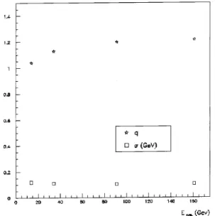
0 (pT > T0) (87) where is the distribution of the transverse momenta pT, T0 is a characteristic temperature which Hagedorn predicts to be independent from the electron-positron collision energy W in the mass center referential, and c is a constant. This theory ts the data quite well for small W, say W < 10 Gev, but exhibits a pronounced failure for W increasing up to say 160 Gev. Very re-cently, Bediaga, Curado and Miranda[102] have used, along Hagedorn's lines, the present generalized statis-tics. The results are indicated in Figs. 8 and 9. Remark that (i) q varies smoothly and monotonically with vary-ing W (Hagedorn's theory is recovered in the W ! 0 limit), and (ii) T0
' 0:11 Gev and practically inde-pends from W as desirable from Hagedorn's arguments. These results can be considered as a strong evidence of the applicability of the nonextensive thermostatistics to specic anomalous systems.
IV.7 Emulsion chamber observation of cosmic
rays
measurements done at the Mount Pamir lead cham-bers) . This distribution was recently tted by Wilk and Wlodarcsyc[105] with the q = 1:3 function which emerges within the present formalism.
Figure 8. Distribution of the transverse momenta p T
ob-tained in electron-positron frontal collisions of energy W
varying from 14 to 161Gev. The dotted line corresponds to q= 1 (i.e., a Hagedorn type of tting as given by Eq. (87))
for all values of W. The solid lines correspond to q 6= 1
ttings.
Figure 9. The values of q and T0 used in the ttings of
Fig. 8. WhenW approaches zero,qapproaches unity, i.e.,
Hagedorn's theory; T0 is essentially insensitive to W, as
physically desirable.
IV.8 Reassociation of heme-ligands in folded
proteins
In the folded conformational state, proteins might exhibit fractal eects. One such case might be the
time evolution of the re-association of molecules that have been taken away from their natural positions. For instance, if O
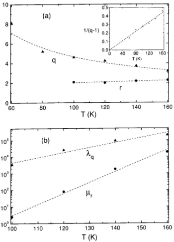
2 molecules are dissociated, through light ashes, from their naturalFepositions in a heme protein and reach positions outside the heme pocket, they tend to start rebinding, and, for so doing, they might have to follow a fractal path, or be under the dynamical inuence of fractal excitations (e.g., frac-tons). Anyhow, this re-association phenomenon has been lengthily studied by Frauenfelder et al[106]. If we dene N(t)=N(0) where N(t) is the number of molecules that have not yet re-associated at timet, the(t) monotonically vanishes witht. The results ob-tained by photo-dissociatingCOmolecules from Sigma Type 2 sperm whale Myoglobin (Mb) dissolved in a glycerol-water solution are shown in Fig. 10. For times not too long, the experimental data have been tted by Frauenfelder et al[106] with
= (1 +t=t 0)
,n (88)
where t 0 and
n smoothly depend on the temperature T. Bemski, Mendes and myself[107] have argued that, within the generalized formalism, the following equa-tion naturally appears:
d dt
=,
q
q (
q
0; q1) (89)
Its solution is given by
=
1 [1 + (q,1)
q t]
1 q ,1
(90)
This expression recovers, for q = 1, the usual ex-ponential relaxation, and reproduces the Frauenfelder form through the identications 1=(q,1) n and 1=[(q,1)
q] t
0. Besides reobtaining the Frauenfelder empiric law, the present scheme allows for a better ap-proximation if a crossover is admitted. More precisely, the above dierential equation can be generalized as follows:
d dt
=,
r
r ,(
q ,
r)
Figure 10. Time evolution of N(t)=N(0) associated
with MbCO in glycerol-water. Dots: experimental data.
Dashed lines: ttings with Frauenfelder's empiric law (Eq. (88) or Eq. (90)). Solid lines: ttings with the solutions of Eq. (91) (see Fig. 11).
Figure 11. Temperature dependences of the parameters used to t the experimental data of Fig. 10.
IV.9 DiusionofHydraVulgaris
Upadhyaya et al[108] are presently performing in-teresting experiments onHydraVulgaris(a cylindrical body column with inner and outer cells, respectively re-ferred to as endodermal and ectodermal respectively) in
physiological solution. The endodermal cells are more adhesive than the ectodermal ones. The authors have measured the velocity distribution P(jV
y
j) of the \ver-tical" component of the velocity during the diusion of endodermal Hydra cells in an ectodermal aggregate. The results are presented in Fig. 12, where the velocity unit is 10,6m=hour and the probability is represented by the histogram of the number of counts. These results were tted with
P(jV y
j) = a (1 + bjV
y j
2)c (92)
with the values of (a;b;c) indicated in the gure. Through the identication
a = P(0); b = (q,1)=V 2
0; c = q q,1
(93) we precisely have the law which emerges within the present formalism, namely
P(jV y
j) =
P(0) [1 + (q,1)(V
y=V0)
2]q =(q ,1) (94) with q = 1:53. The next desirable step of course is to formulate a specic model for Hydra which would lead to this law, but this remains to be done.
IV.10 Citationof scienticpap ers
An interesting study was recently done by Redner[109], in which the statistics of citations of scien-tic papers is focused. He exhibited the number N(x) of papers which have been cited x times for two long se-ries, namely one (6 716 198 citations of 783 339 papers) from the Institute of Scientic Information (ISI) and another one (351 872 citations of 24 296 papers) from the Physical Review D (PRD). As expected, in both examples, N(x) monotonically decreases with x. Red-ner tted the (relatively) low-x data with a stretched exponential of the form
N(x) = N(0) e,(x=x0)
(95) with = 0:44 and 0:39 for the series ISI and PRD respectively. Also, he remarked that the large-x data exhibit a power law, namely close to/1=x
these two regimes. In contrast with this viewpoint, Al-buquerque and myself[110] argue that this is not neces-sarily so since the data can be quite satisfactorily tted with asinglefunction, namely
N(x) =
N(0) [1 + (q,1)x]
q =(q ,1) (96)
with q= 1:53 and 1:64 for the series ISI and PRD re-spectively: see Fig. 13 The satisfactory quality of the ttings is, after all, not so surprising, since we have mentioned earlier in this paper the connection[84] of this formalism with the Zipf law.
Figure 12. Distribution of the \vertical" velocities during diusion of endodermal Hydra cells in an ectodermal aggre-gate. The abcissa units are 10,6 m=hour. The tting was
obtained using q= 1:53 (see the text).
Figure 13. Distribution of ISI and PRD papers having received xcitations. (a) and (b) exhibit the ttings in [109]; (c) and (d) exhibit our present ttings (see the text).
IV.11 Electro encephalographic signals of epilepsy
It is since long known that the analysis of sig-nals can be done within formalisms which use entropic forms. One such application has been recently done on EEG records of epilleptic humans and turtles[111].
The simultaneous use of wavelet-based multiresolution analysis including the nonextensive entropy S
IV.12 Cognitive psychology
The development of articial neural networks and their connections with statistical mechanics (e.g., the Hopeld model for associative memory) makes quite natural the approach of cognitive problems with the present nonextensive formalism. Within this phi-losophy, we performed[112] an experiment of learn-ing/memorization (of 55 and 77 square matrix having circles and crosses randomly distributed once for ever) with students of the University level; 150 stu-dents were interviewed, the rst 30 in order to opti-mize the experimental protocole, and the other 120 to make the measurements of the time-evolution of the to-tal amounts of errors when the original matrix was suc-cessively shown and hidden. The average results were then tted with those obtained, for the same task, with a learning machine[113] having a perceptron architec-ture and an internal dynamics based on the Langevin equation[44] generalized by Stariolo to arbitraryq. The (average) learning time of the machine turned out to monot onically increase withq, exhibiting a practically divergent derivative atq= 1. The best human-machine t occurred for q slightly above unity. More experi-ments and comparisons along these lines would be very welcome. Indeed, they would help better understanding some cognitive phenomena, on one hand, and could gen-erate ecient machines for specic tasks, on the other.
IV.13 Turbulence and time evolutionof nancial
data
In 1996 Ghashghaie et al[114] compared nancial data with those obtained from turbulent behavior and showed very similar behaviors when appropriate scal-ings are used. Ramos et al[115] have recently shown that all these data can be satisfactorily tted with the functional form which emerges from the present for-malism. Olsen and Associates data containing bid-ask quotes for US dollar-German mark exchange rates (1,472,241records) are presented in Fig. 14 (probability densityP
t(
) of price changes; =(t), (t+t) with t= 640s; 5120s; 40960s; 163840sfrom top to bottom in the gure). The turbulent ow data[116] are presented in Fig. 15 (probability density P
r(
v) of velocity dierences; v=v(r),v(r+ r) for spatial scale delays r= 3:3 ; 18:5 ; 138 ; 325from top to
bottom in the gure, where is the Kolmogorov scale, i.e., the critical limit for occurence of viscous dissipa-tion). All these data exhibit a slight left-right assym-metry, which has been taken into account by Ramos et al: they used the same q for both sides but dierent widths. Needless to say that specic models leading to these tting functions are very welcome.
Figure 14. Distributions of price changes for US dollar-German mark exchange rates and ttings using assymetric
q-distributions (see the text).
V Computational
evidences
and connections
V.1 Thermalization of a hot gas penetrating in
a cold gas
In 1991, Waldeer and Urbassek[117] made, assuming d = 3 Newtonian mechanics, a computational simula-tion in which a certain amount of high energy particles penetrate into a cold gas and are thermalized through the interactions between molecules. The cold gas is ini-tially put at BG thermal equilibrium at temperature TC. The high energy particles at time t = 0 are ran-domly distributed in energy at a quite high energy per particle. The interaction potential was assumed to be hard sphere at short distances and decreasing, at long distances, like r,. They analyzed three typical situa-tions, one with !1, hence well above d (i.e., very short range interactions), the second one with = 4 (i.e., short range interactions), and the last one with = 8=3, which is below d (i.e., long range interac-tions). In their simulation, they follow the time evo-lution of the energy distribution of the hot particles. After a transient, this distribution evolves with a regu-lar pattern. For > d, this pattern basically is the BG distribution with a temperature T(t) which gradually approaches TC from above (with limt!1T(t) = TC), in other words, through curves which approximatively are straight lines in a log-linear plot. For < d, this approximation occurs through curves which are close to straight lines... in a log-log plot. (Notice that the cur-vature in log-log plots tends to be upwardsfor < d, whereas it is downwards for > d; see Figs. 1, 2 and 3 of [117]). This power-law behavior is typical of q > 1. This pecualiarity was invoked by Koponen[9] in 1997 as a justication for using the present generalized formalism to discuss electron-phonon relaxation in ion-bombarded solids if the interactions are long-ranged. A study like that of Waldeer and Urbassek[117] which would systematically address the details of that ther-malization by gradually varying across d is missing and would certainly be very welcome.
V.2 Long-range classical Hamiltonian systems:
Static properties
Let us focus here on what we refer to asweak vio-lation of BG statistics. We use this expression to dis-tinguish it from what we call strong violation of BG
statistics. Both of them lead to nonextensive quanti-ties, but, whereas the strong violation concerns q6= 1, the weak one concerns q = 1 calculations. To make all this explicit we shall here focus on classical systems, i.e., all observables are assumed to commute. Let us consider the following paradigmatic Hamiltonian:
H = 12m N X i=1
p2 i +
X i6=j
V (rij) (97) where m is a microscopic mass, fp
i;ri
g are the d-dimensional linear momenta and positions associated with N particles, and rij
r j
,r
i. A typical situation is that of a nite conned system but, if some care is taken, the system could as well be thought of as hav-ing periodic boundary conditions. To be specic, let us assume
V (rij) = A r12
ij ,
B r ij
(A > 0;B > 0;0 < 12) (98) where, in order to avoid any singularity at the origin (for any dimension d not exceedingly high), we have assumed, for the repulsive term, the Lennard-Jones ex-ponent 12. What we desire to focus on in the present discussion is possible singularities associated with in-nite distances, i.e., the eects of long-range (attrac-tive) interactions. The case (;d) = (6;3) precisely recovers the standard Lennard-Jones uid; the case (;d) = (1;3) is asymptotically equivalent to Newto-nian gravitation; the case (;d) = (d,2;d) is asymptot-ically equivalent to d-dimensional gravitation (i.e., the one associated with the solutions of the d-dimensional Poisson equation); the case (;d) = (3;3) basically re-produces the distance dependance of permanent dipole-dipole interaction. The range of the (attractive) inter-action increases when decreases; !12 corresponds to very short-ranged interactions, whereas = 0 corre-sponds to the situation of the Mean Field A pproxima-tion, where every particle (attractively) interacts with every other with thesamestrength, in all occasions.
A typical quantity to be calculated within BG statis-tics is the following one (basically related to the T = 0 internal energy per particle):
Z 1 1
dr rd,1 r,


![Figure 5. The one-jump distributions pq ( x ) for typical values of q . The q ! ,1 distribution is the uniform one in the interval [ , 1 ; 1]; q = 1 and q = 2 respectively correspond to Gaussian and Lorentzian distributions; the q ! 3 is completely at](https://thumb-eu.123doks.com/thumbv2/123dok_br/18978563.456186/10.918.217.753.215.574/distributions-distribution-respectively-correspond-gaussian-lorentzian-distributions-completely.webp)


![Figure 13. Distribution of ISI and PRD papers having received x citations. ( a ) and ( b ) exhibit the ttings in [109]; ( c ) and ( d ) exhibit our present ttings (see the text).](https://thumb-eu.123doks.com/thumbv2/123dok_br/18978563.456186/21.918.211.703.519.902/figure-distribution-papers-received-citations-exhibit-exhibit-present.webp)

