known cases, for sums and maxima of uncorrelated and correlated random variables. I recall why several of them appear in physics. Next, I show that there is room for new versions of central limit theorems applicable to specific classes of problems. Finally, I argue that we have insufficient evidence that, as a consequence of such a theorem,q-Gaussians occupy a special place in statistical physics.
Keywords: Central limit theorems, Sums and maxima of correlated random variables,q-Gaussians
Central limit theorems play an important role in physics, and in particular in statistical physics. The reason is that this discipline deals almost always with a very large numberN of variables, so that the limitN→∞required in the mathe-matical limit theorems comes very close to being realized in physical reality. Before looking at some hard questions, let us make an inventory of a few things we know.
1. SUMS OF RANDOM VARIABLES
Gaussians and why they occur in real life
Let p(x) be an arbitrary probability distribution of zero mean. Draw from it independentlyNvariablesx1,x2, . . . ,xN and then ask what is the probabilityPN(Y)that the scaled sum
(x1+x2+. . .+xN)/N1/2 take the valueY. The answer, as we explain to our students, is obtained by doing the convolu-tionPN(Y) =p(x1)∗p(x2)∗···p(xN). After some elementary rewriting one gets
PN(Y) = 1 p
2πhx2iexp
− Y
2
2hx2i+ 1 N1/2
. . .
, (1)
where the dots stand for an infinite series of terms that depend on all moments ofp(x)higher than the second one,hx3i,hx4i, . . . . In the limitN→∞the miracle occurs: the dependence on these moments disappears from (1) and we find the Gaussian P∞(Y) = (2πhx2i)1/2exp −12Y2/hx2i.
The important point is that even if you didn’t know before-hand about its existence, this Gaussian results automatically from any initially given p(x)– for example a binary distri-bution with equal probability forx=±1. This is the Central Limit Theorem (CLT); it says that the Gaussian is an attrac-tor [1]under addition of independent identically distributed random variables. An adapted version of the Central Limit Theorem remains true for sufficiently weakly correlated vari-ables.
This theorem of probability theory is, first of all, a mathematical truth. In order to see why it is relevant to real
∗Electronic address:[email protected]
†text at the basis of a talk presented at the 7th International
Confer-ence on Nonextensive Statistical Mechanics: Foundations and Applications (NEXT2008), Foz do Iguac¸u, Paran´a, Brazil, 27-31 October 2008.
life, we have to examine the equations of physics. It appears that these couple their variables, in most cases, only over short distances and times, so that the variables are effectively independent. This is the principal reason for the ubiquitous occurrence of Gaussians in physics (Brownian motion) and beyond (coin tossing). Inversely, the procedure of fitting a statistical curve by a Gaussian may be considered to have a theoretical basis if the quantity represented can be argued to arise from a large number of independent contributions, even if these cannot be explicitly identified.
L´evy distributions
Symmetric L´evy distributions. Obviously the calculation leading to (1) requires that the variancehx2ibe finite. What if it isn’t? That happens, in particular, when forx→ ±∞the distribution behaves asp(x)≃c±|x|−1−αfor someα∈(0,2). Well, then there is a different central limit theorem. The attractor is a L´evy distributionLα,β(Y), whereY is again the sum of the xn scaled with an appropriate power of N and where β∈(0,1) depends on the asymmetry between the amplitudesc+ andc−. A description of the Lα,β is given,
e.g., by Hughes ([2], see § 4.2-4.3). In the symmetric case c+=c−we haveβ=0. ThenL1,0(Y)is the Lorentz-Cauchy distributionP∞(Y) =1/[π(1+Y2)]andL2,0(Y)is the Gaus-sian discussed above.
Asymmetric L´evy distributions. Ifc−=0, that is, if p(x)
has a slow power law decay only for large positive x, then we haveβ=1 and the limit distribution is theone-sided L´evy distribution. In the special caseα=12, shown in Fig. 1, we have the Smirnov distributionL1
2,1. It has the explicit analytic
expression
P∞(Y) =√ 1 4πY3exp
− 1
4Y
, Y>0, (2)
and decays for largeY as∼Y−3/2.
All these L´evy distributions are attractors under addition of random variables, just like the Gaussian, and each has its own basin of attraction.
Addition of nonidentical variables
inde-FIG. 1: The one-sided L´evy distributionL1 2,1(
Y)is one possible out-come of a central limit theorem.
FIG. 2: A sequence of probability distributions developing a “fat tail” proportional to∼τ−3/2whenk→∞.
pendent butnon-identical variables. If they’re not too non-identical, you still get Gauss and L´evy distributions. The pre-cise premises (the “Lindeberg condition”), under which the sum of a large number of nonidentical variables is Gaussian distributed, may be found in a recent review for physicists by Clusel and Bertin [3].
Now consider a case in which the Lindeberg condition does not hold. Suppose a distribution p∞(τ), defined for τ>0, decays asτ−3/2in the large-τlimit. Let it be approximated, as shown in Fig. 2, by a sequence of truncated distributions p1(τ),p2(τ), . . . ,pk(τ), . . .which is such that in the limit of largekthe distribution pk(τ)has its cutoff atτ∼k2. Then how will the sumtL≡τ1+τ2+. . .+τLbe distributed?
The answer is that it will be a bell-shaped distribution which is neither Gaussian nor asymmetric L´evy, but some-thing in between. It’s given by a complicated integral that I will not show here. It is again an attractor: it does not depend on the shape ofp(τ)and thepk(τ)for finiteτ, but only on the asymptotic large-τbehavior of these functions as well as on how the cutoff progresses for asymptotically largek.
An example: support of 1D simple random walk. An ex-ample of just these distributions occurs in the following not
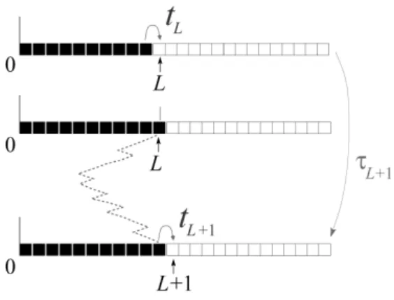
FIG. 3: A random walker on the positive half-line pays its first visit to siteLat timetL. The sites (squares) already visited are colored
black. The time interval between the first visits toL and toL+
1 is equal toτL+1. During this time interval the walker makes an excursion in the direction of the origin, as indicated by the dotted trajectory. The probability distributionspL(τL)are independent but
non-identical.
totally unrealistic situation, depicted in Fig. 3, and which was studied by Hilhorst and Gomes [4]. A random walker on a one-dimensional lattice with reflecting boundary conditions in the origin visits siteLfor the first time at timetL. We can then writetL=τ1+τ2+. . .+τL, whereτkis the time differ-ence between the first visit to the(k−1)th site and thekth site. Askincreases, theτktend to increase because of longer and longer excursions inside the region already visited. Theτkare independent variables of the type described above. ForL→∞ the probability distribution oftLtends to an asymmetric bell-shaped function of the scaling variabletL/L2which is neither Gaussian nor L´evy. It is given by an integral that we will not present here. It is universal in the sense that it depends only on the asymptotic largeτbehavior of the functions involved.
Sums having a random number of terms
The game of summing variables still has other variations. We may, for example, sumNi.i.d. whereNitself is a random positive integer. LetNhave a distributionπN(ν)whereνis a continuous parameter such thathNi=ν. Then forν→∞ one easily derives new variants of the Central Limit Theorem.
2. MAXIMA OF RANDOM VARIABLES
Gumbel distributions
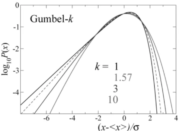
FIG. 4: The Gumbel-kdistribution for various values ofk.
is easily written down as an integral,
PN(Y) = d dY
1−
Z ∞
Y d x p(x)
N
. (3)
The calculation is a little harder to do than for the case of a sum. Let us subject the variableY to an appropriate (and generallyN-dependent) shift and scaling and again call the resultY. Then one obtains
P∞(Y) =e−Ye−e −Y
, (4)
which is the Gumbel distribution.
The asymptotic decay of p(x) was supposed here faster than any power law. If it is as a power law, a different dis-tribution appears, called Fr´echet; and if p(x)is strictly zero beyond some cutoffx=xc, a third distribution appears, called Weibull. Again, mathematicians tell us that for this new ques-tion these three cases exhaust all possibilities.
In Ref. [3] an interesting connection is established between distributions of sums and of maxima.
The Gumbel-k distribution.The Gumbel distribution (4) is depicted in Figs. 4, where it is called “Gumbel-1”. This is because we may generalize the question and ask not how the largest one of thexi, but how thekth largest one of them is distributed? The answer is that it is a Gumbel distributionof index k. Its analytic form is known and containskas a param-eter. Fork→∞it tends to a parabola, that is, to a Gaussian.
All these distributions areattractors under the maximum operation. Even if you did not know them in advance, you would be led to them starting from an arbitrary given distri-butionp(x)within its basin of attraction.
Bertin and Clusel [5, 6] show that the definition of the Gumbel-k distribution may be extended to real k. These authors also show how Gumbel distributions of arbitrary index k may be obtained as sums of correlated variables. Their review article [3] is particularly interesting.
The BHP distribution
In 1998 Bramwell, Holdsworth, and Pinton (BHP) [7] adopted a semi-empirical approach to the discovery of new
FIG. 5: The Gumbel-1 and the BHP distribution.
universal distributions. These authors noticed that, within er-ror bars,exactly the same probability distributionis observed for (i) the experimentally measured power spectrum fluctu-ations of 3D turbulence; and (ii) the Monte Carlo simulated magnetization of a 2D XY model on anL×Llattice at tem-peratureT<Tc, in spin wave approximation.
For the XY model Bramwellet al. [8, 9] were later able to calculate this distribution. It is given by a complicated integral that I will not reproduce here and is called since the “BHP distribution.” Fig. 5 shows it together with the Gumbel-1 distribution [10].
Numerical simulations. How universal exactly is the BHP distribution? Bramwellet al.[8] were led to hypothesize that the BHP occurs whenever you look for the maximum of, not independent, butcorrelated variables. To test this hypothesis these authors generated a random vector~x= (x1, . . . ,xN)of N elements distributed independently according to an expo-nential, and acted on it with a fixed random matrixM such as to obtain~y=M~x. By varying~xfor a single fixedMthey obtained the distribution ofY =max1≤i≤Nyiand concluded that indeed it was BHP.
However, Watkins et al. [11] showed one year later by an analytic calculation that what appears to be a BHP distri-bution in reality crosses over to a Gumbel-1 law whenN is increased. In this case, therefore, the correlation is irrelevant and the attractor distribution is as for independent variables.
Watkinset al. conclude that “even though subsequent re-sults may show that the BHP curvecan result from strong correlation, itneed not.” This example illustrates the danger of trying to attribute an analytic expression to numerically ob-tained data.
In later work Clusel and Bertin [3] present heuristic arguments tending to explain why distributions closely resembling the BHP distribution occur so often in physics.
Wider occurrence of Gumbel and BHP?
Gumbel-6 distribution ([12], Fig. 4b).
Gonc¸alves and Pinto [13] consider the distribution of the cp daily return of two stock exchange indices (DJIA30 and S&P100) over a 21 year period. They find that the cubic root of the square of this distribution is extremely well fitted by the BHP curve ([13], Figs. 1 and 2).
In both cases the authors are right to point out the qual-ity of the fit. But these examples also show that having a very good fit doesn’t mean you have a theoretical explanation.
3. CORRELATED VARIABLES
In addition to the example discussed above, we will provide here two further examples of how the maximum of a set of correlated random variables may be distributed. These examples will illustrate the diversity of the results that emerge.
Airy distribution. Fig. 6 shows the trajectory of a one-dimensional random walker in a given time interval, subject to the condition that the starting point and end point coin-cide. The walker’s positions on two different times are clearly correlated. Letxdenote the maximum deviation (in absolute value) of the trajectory from its interval average.
Majumdar and Comtet [14] were able to show that this maximum distance is described by the Airy distribution (distinct from the well-known Airy function), which is a weighted sum of hypergeometric functions that I will not reproduce here. It is again universal: Schehr and Majumdar [15] showed in analytic work, supported by numerical simu-lations, that this same distribution appears for a wide class of walks with short range steps. It turns out [14], however, that the distribution changes if the periodic boundary condition in time is replaced by free boundaries. This therefore puts a limit on the universality class [1].
Magnetization distribution of Ising 2D at criticality. We consider a finiteL×L two-dimensional Ising model with a set of short-range interaction constants{Jk}. Its magnetiza-tion (per spin) will be denotedM=N−1∑iN=1si, whereN=L2 and thesi are the individual spins. We ask what the distri-butionPL(M)is exactlyat the critical temperatureT =Tc. This distribution can be determined, in principle at least, by a
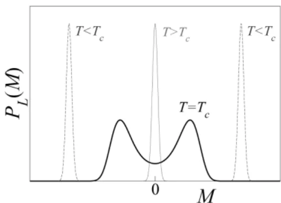
FIG. 7: Qualitative behavior of the distributionPL(M)of the
magne-tization of the 2D Ising model on a periodicL×Llattice. The sharp peaks forT >TcandT<Tcare Gaussians. ForT=Tcand under suitable scalingPL(M)tends in the limitT→∞to a double-peaked
universal distributionP(m); see Eq. (5) and the accompanying text.
renormalization calculation which in its final stage gives
L−18PL(M) =
P
m,{L−yℓuℓ}, (5)
wherem=L18M and where{yℓ} is a set of positive
fixed-point indices with corresponding scaling fields{uℓ}(i.e. the uℓ are nonlinear combinations of theJk). In the limit L→ ∞the dependence on these scaling fields disappears and we have, in obvious notation, that limL→∞L−
1
8PL(M) =
P
(m).In Fig. 7 the distributionPL(M)is depicted qualitatively for L≫1 (it has two peaks!), together with the Gaussians that prevail whenT 6=Tc. The reason forM not being Gaussian distributed exactly at the critical point is that forT =Tc the spin pair correlation does not have an exponential but rather a slow power law decay with distance: the spins are strongly correlated random variables.
The similarity between Eq. (5) and Eq. (1) is not fortuitous: the coarse-graining of the magnetization which is implicit in renormalization, amounts effectively to an addition of spin variables; and the set of irrelevant scaling fields{uℓ}plays the same role as the set of higher moments{hxni|n≥3}in Eq. (1).
Eq. (5) says that
P
(m) is an attractor under the renor-malization group flow; it is reached no matter what set of coupling constants{Jk}was given at the outset. Here, too, there are limits on the basin of attraction: the shape ofP
(m)depends, in particular, on the boundary conditions (periodic, free, or otherwise [16]).
The conclusion from everything above is that attractor dis-tributions come in all shapes and colors, and that it makes sense to try and discover new ones.
4. q-GAUSSIANS
Aq-Gaussian Gq(x)is the power of a Lorentzian, Gq(x) =
cst
[1+ax2]p=
cst
[1+ (q−1)x2]q−11
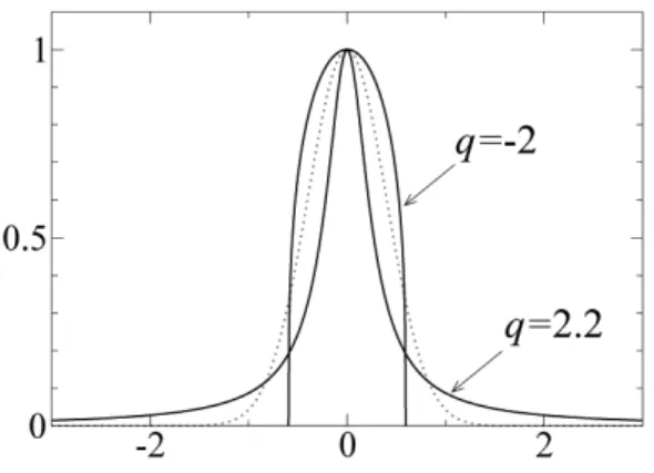
FIG. 8: Examples ofq-Gaussians. Dotted curve: the ordinary Gaus-sian,q=1. Solid curves: theq-Gaussians forq=2.2 andq=−2; the former has fat tails whereas the latter is confined to a compact support. All three curves are normalized to unity in the origin.
where in the second equality we have set p=1/(q−1)and scaled xsuch that a=q−1. Examples of q-Gaussians are shown in Fig. 8. Forq=2 the q-Gaussian is a Lorentzian; in the limit q→1 it reduces to the ordinary Gaussian; for q<1 it is a function with compact support, defined only for −xm<x<xmwherexm=1/√1−q. Forq=0 it is an arc of a parabola and forq→ −∞(with suitable rescaling ofx) it tends to a rectangular block.
Interest inq-Gaussians in connection with central limit the-orems stems from the fact that they have many remarkable properties that generalize those of ordinary Gaussians. One may consider, for example, the multivariate q-Gaussian ob-tained by replacingx2in (6) with ∑n
µ,ν=1xµAµνxν (withAa symmetric positive definite matrix). Upon integrating this q-Gaussian on mof its variables we find that the marginal
(n−m)-variable distribution isqm-Gaussian withqm=1− 2(1−q)/[2+m(1−q)] (see Vignat and Plastino [17]; this relation seems to have first appeared in Mendes and Tsallis [18]).
A special case is the uniform probability distribution inside ann-dimensional sphere of radiusR,
Pn(x1, . . . ,xn) =cst×θ R2− n
∑
µ=1x2µ
!
, (7)
whereθdenotes the Heaviside step function. This is actually a multivariateq-Gaussian withq=−∞. Integrating onmof its variables yields aq-Gaussian withqm=1−2/m. We see that for largemboth in the general and in the special caseqm approaches unity and hence these marginal distributions tend under iterated tracing to an ordinary Gaussian shape.
Let us first see, now, how q-Gaussians may arise as solutions of certain partial differential equations in physics.
Differential equations andq-Gaussians
Thermal diffusion in a potential. The standard Fokker-Planck (FP) equation describing a particle of coordinatex
dif-1/kBT. For the special choice of potentialU′(x) =αx/(1+ γx2)the stationary distribution becomes theq-Gaussian
PUst(x) =cst× 1+γx2−αβ/γ
. (9)
This distribution is anattractor under time evolution,the lat-ter being defined by the FP equation (8); a large class of rea-sonable initial distributions will tend to (9) ast→∞[19]. It should be noted, however, that by adjustingU(x)we may obtain any desired stationary distribution, and hence theq -Gaussian of Eq. (9) plays no exceptional role.
The following observation is trivial but will be of interest later on in this talk. Letx(t)be the Brownian trajectory of the diffusing particle. Letx(0)be arbitrary and letx(t), fort>0, be the stochastic solution of the Langevin equation associated [20] with the FP equation (8). Letξn=x(nτ)−x((n−1)τ), whereτis a finite time interval. ThenYN=ξ1+ξ2+. . .+ξN (without any scaling) is a sum which for N →∞ has the distributionPst
U(Y). In particular, ifU(x)is chosen such as to yield (9), we have constructed aq-Gaussian distributed sum.
Finite difference scheme [21]. Rodr´ıguez et al.[22] re-cently studied the linear finite difference scheme
rN,n+rN,n+1=rN−1,n, (10) whereN=0,1,2, . . .andn=0,1, . . . ,N. The quantitypN,n≡
N n
rN,nmay be interpreted as the probability that a sum of N identical correlated binary variables be equal to n. For specific boundary conditions, the authors were quite remark-ably able to find a class of analytic solutions to Eq. (10) and observed that the N→∞limit of the sum law pN,n is aq -Gaussian.
To understand better what is happening here, let us set t=1/N,x=1−2n/N, andP(x,t) =N Nn
rN,n. When ex-panding Eq. (10) in powers ofN−1 one discovers [23] that P(x,t)satisfies the Fokker-Planck equation
∂P(x,t)
∂t = 1 2
∂2 ∂x2
(1−x2)P
(11)
fort >0 and−1<x<1. The “time” t runs in the direc-tion ofdecreasing N. Hence Rodr´ıguezet al. have solved a parabolic equation backward in time and determined, starting from the small-Nbehavior, what is actually aninitial condi-tion atN=∞. It is obvious thatq-Gaussians are not singled out here: there exists a solution to Eq. (11) for any other ini-tial condition att=0, and concomitantly to Eq. (10) for any desired limit functionp∞,natN=∞.
however possible to find special classes of solutions. One special solution is obtained by looking for solutions that are (i) radially symmetric,i.e.,dependent only onx≡ |~x|; and (ii) scale asu(~x,t) =t−dbF(xt−b). After scaling of xandt we obtain the similarity solution
ρ(~x,t) = c0
tdb
1+ (q−1)x
2
t2b −q−11
, (13)
in whichb=1/[d(1−q) +2]and where alsoc0is uniquely defined in terms of the parameters of the equation. Mathe-maticians (seee.g.[24]) have shown that initial distributions with compact support tend asymptotically towards this simi-larity solution. The asymptotic behavior (13) is conceivably robust, within a certain range, against various perturbations of the porous medium equation. It is not clear to me if and how this property can be connected to a central limit theorem.
q-statistical mechanics
Considerations from aq-generalized statistical mechanics [25–27] have led Tsallis [28] to surmise that in the limitN→ ∞the sum ofN correlated random variables becomes, under appropriate conditions,q-Gaussian distributed; that is, on this hypothesisq-Gaussians are attractors in a similar sense as or-dinary Gaussians. Now, variables can be correlated in very many ways. To fully describeNcorrelated random variables you need theN variable distributionPN(x1, . . . ,xN). Taking the limitN→∞requires knowing theset of functions
PN(x1, . . . ,xN), N=1,2,3, . . . (14) In physical systems the PN are determined by the laws of nature; the relative spatial and/or temporal coordinates of the variables, usually play an essential role. The examples of the Ising model and of the Airy distribution show how widely the probability distributions of strongly correlated variables may vary. Hence, in the absence of any elements of knowledge about the physical system that they describe, statements of uniform validity about correlated variables cannot be expected to be very specific.
q-Central Limit Theorem
We now turn to aq-generalized central limit theorem (q -CLT) formulated by Umarov et al. [29]. It says, essen-tially, the following. Given an infinite set of random variables
of correlations among its variables.
Secondly, the proof of the theorem makes use of “q-Fourier space,” theq-Fourier transform (q-FT) having been defined in Ref. [29] as a generalization of the ordinary FT. Theq-FT has the feature that when applied to aq-Gaussian it yields aq′ -Gaussian withq′= (1+q)/(3−q), for 1≤q<3. Now the q-FT is a nonlinear mapping which appears not to have an inverse [30]. It is therefore unclear at present how the state-ments of the theorem derived inq-Fourier space can be trans-lated back in a unique way to “real” space.
5. THE SEARCH FORq-GAUSSIANS
Mean-field models
Independently of thisq-CLT Thistletonet al.[31] (see also Ref. [32]) attempted to see aq-Gaussian arise in a numerical experiment. These authors defined a system ofNvariablesxi, i=1,2, . . . ,N, equivalent under permutation. Each variable is drawn from a uniform distribution on the interval(−1
2, 1 2) but thexi are correlated in such a way thathxjxki=ρhx21i for all j6=k, where ρ is a parameter in(0,1) [33]. They considered the sumYN= (x1+. . .+xN)/Nand determined its distributionP(Y)in the limitN≫1. Forρ= 7
10the numerical results forP(Y)can be fitted very well by aq-GaussianGq(Y) withq=−5
9, shown as the dotted curve in Fig. 9. This system of correlated variables is sufficiently simple that Hilhorst and Schehr [34] were able to do the analytic calculation of the distribution. They found thatY is distributed according to
P(Y) =2−ρ
ρ
12
exp−2(1ρ−ρ)
erf−1(2Y)2 , (15)
for−1 2<Y<
1
FIG. 9: Comparison of theq-GaussianGq(Y)(dotted curve) guessed
in Ref. [31] on the basis of numerical data and the exact distribution
P(Y)(Eq. (15), solid curve) calculated in Ref. [34]. The curves are forρ= 7
10and theq-Gaussian hasq=−59. The difference between the two curves is of the order of the thickness of the lines and just barely visible to the eye.
The work discussed here concerns a mean-field type model: there is full permutational symmetry between all variables. This will be different in the last two models that we will now take a look at.
Logistic map and HMF model
Two well-known models of statistical physics have been evoked several times by participants [35, 36] at this meeting. The common feature is that in each of them the variable studied is obtained as an average along a deterministic trajectory.
Logistic map. In their search for occurrences of q -Gaussians in nature, Tirnakliet al. [37] considered the lo-gistic map
xℓ=a−x2ℓ−1, ℓ=1,2, . . . (16) A motivation for this choice is the appearance [38] of q -exponentials in the study of this map. Starting from a uni-formly random initial conditionx=x0, Tirnakliet al. deter-mined the probability distribution of the sum
Y =
n0+N
∑
ℓ=n0xℓ (17)
of successive iterates, scaled with an appropriate power of N, in the limit N≫1. Their initial report of q-Gaussian behavior at the Feigenbaum critical point (defined by a critical value a =ac) was critized by Grassberger [39]. Inspired by a detailed study due to Robledo and Mayano [40], who connect propertiesat a=acto properties observed onapproaching this critical point, Tirnakliet al. [41] took a renewed look at the same question and now see indica-tions for aq-Gaussian distribution ofY nearthe critical point.
∑
i 2 2L
∑
i,jwhere pi andθi are the momentum and the polar angle, re-spectively, of theith mass. The angles were originally con-sidered to describe the state of classical XY spins, so that ~
mi= (cosθi,sinθi)is the magnetization of theith spin. The HMF has a solvable equilibrium state. At a critical value U=Uc=0.75 of the total energy per particle a phase transi-tion occurs from a high-temperature state with uniformly dis-tributed particles to a low-temperature one with a spontaneous value of the “magnetization”h|M~|i, whereM~ =L−1∑Li=1~mi. When launched with certain nonequilibrium initial condi-tions, the system, before relaxing to equilibrium, appears to enter a “quasi-stationary state” (QSS) whose lifetime diverges withN. It is impossible to discuss here all the good work that has been done, and is still going on, to attempt to explain the properties of this state (seee.g. Chavanis [43–45], Tsalliset al. [46], Antoniazziet al. [47], Chavaniset al. [48]). One specific type of numerical simulations, performed by differ-ent groups of authors, is relevant for this talk. These have been performed at the subcritical energyU=0.69 with ini-tially all particles located at the same point (θi=0 for alli) and the momentapidistributed randomly and uniformly in an interval[−pmax,pmax]. The QSS subsequent to these initial conditions has many features (such as non-Gaussian single-particle velocity distributions) that have been connected toq -statistical mechanics. Of fairly recent interest is the sumYi of the single-particle momentum pi(t)sampled at regularly spaced timest=ℓτalong its trajectory,
Yi= n0+N
∑
ℓ=n0pi(ℓτ). (19)
The distribution ofYi in the limit of large N is again con-troversial [49, 50]. For the specific initial conditions cited above it seems to first approach a fat-tailed distribution, interpreted by some as aq-Gaussian, before it finally tends to an ordinary Gaussian.
[1] In certain contexts attractors are also calleduniversal distribu-tions.In this talk the two terms will be used interchangeably. Concomitantly, “basin of attraction” and “universality class” will denote the same thing here.
[2] B.D. Hughes,Random Walks and Random Environments,Vol. 1:Random Walks,Clarendon Press, Oxford (1995).
[3] M. Clusel and E. Bertin,arXiv:0807.1649.
[4] H.J. Hilhorst and Samuel R. Gomes Jr. (1998),unpublished.
[5] E. Bertin,Phys. Rev. Lett.95(2005) 170601. [6] E. Bertin and M. Clusel,J. Phys. A 39(2006) 7607.
[7] S.T. Bramwell, P.C.W. Holdsworth, and J.-F. Pinton,Nature
396(1998) 552.
[8] S.T. Bramwell, K. Christensen, J.-Y. Fortin, P.C.W. Holdsworth, H.J. Jensen, S. Lise, J.M. L´opez, M. Nicodemi, J.-F. Pinton, and M. Sellitto,Phys. Rev. Lett.84 (2000) 3744.
[9] S.T. Bramwell, Y. Fortin, P.C.W. Holdsworth, S. Peysson, J.-F. Pinton, B. Portelli, and M. Sellitto,Phys. Rev. E 63(2001) 041106.
[10] The BHP curve is in fact very close to the Gumbel-k distribu-tion withk=1.57 shown in Fig. 4.
[11] N.W. Watkins, S.C. Chapman, and G. Rowlands,
Phys. Rev. Lett.89(2002) 208901. [12] M. Palassini,J. Stat. Mech.(2008) 10005. [13] R. Gonc¸alves and A.A. Pinto,arXiv:0810.2508.
[14] S. Majumdar and A. Comtet, Phys. Rev. Lett. 92 (2004) 225501.
[15] G. Schehr and S. Majumdar,Phys. Rev. E73(2006) 056103. [16] Indeed,P(m)has been determined for Ising models on surfaces
topologically equivalent to a M¨obius strip and a Klein bottle! See K. Kaneda and Y. Okabe,Phys. Rev. Lett.86(2001) 2134. [17] C. Vignat and A. Plastino,Phys. Lett. A365(2007) 370. [18] R.S. Mendes and C. Tsallis,Phys. Lett. A285(2001) 273. [19] Forγ→0 the force−U′(x)is linear and we recover from (9)
the ordinary Gaussian, that is, the equilibrium distribution in a harmonic potential.
[20] N.G. van Kampen,Stochastic Processes in Physics and Chem-istry, North-Holland, Amsterdam (1992).
[21] Paragraph added after the Conference.
[22] A. Rodr´ıguez, V. Schw¨ammle, and C. Tsallis, J. Stat. Mech.
(2008) P09006.
[23] H.J. Hilhorst (2009), unpublished.
[24] J.L. V´azquez, The Porous Medium Equation: Mathematical Theory, Oxford University Press, Oxford (2006).
[25] C. Tsallis,J. Stat. Phys.52(1988) 479.
[26] M. Gell-Mann and C. Tsallis eds.,Nonextensive Entropy –
In-terdisciplinary Applications,Oxford University Press, Oxford (2004).
[27] C. Tsallis,Introduction to Nonextensive Statistical Mechanics: Approaching a Complex World,Springer, Berlin (2009). [28] C. Tsallis,Milan J. Math.73(2005) 145.
[29] S. Umarov, C. Tsallis, and S. Steinberg, Milan J. Math.76 (2008) xxxx.
[30] Ref. [29] associates with a function f(x) theq-Fourier trans-form ˆfq(ξ) =Rdx f(x)1−(q−1)iξx fq−1(x)−1/(q−1). As an
example let us take f(x) = (λ/x)1/(q−1) in an interval [a,b]
(witha,b,λ>0) and f(x) =0 zero otherwise. Normalization fixesλas a function ofaandb. Then it is easily verified that
ˆ
fq(ξ)is the same for the entire one-parameter family of
inter-vals defined byλ(a,b) =λ0. Hence theq-FT is not invertible on the space of probability distributions. Other examples may be constructed.
[31] W. Thistleton, J.A. Marsh, K. Nelson, and C. Tsallis (2006) un-published; C. Tsallis,Workshop on the Dynamics of Complex SystemsNatal, Brazil, March 2007.
[32] L.G. Moyano, C. Tsallis, and M. Gell-Mann,Europhys. Lett.
73(2006) 813.
[33] The exact procedure that they followed is described in Ref. [34].
[34] H.J. Hilhorst and G. Schehr,J. Stat. Mech.(2007) P06003. [35] U. Tirnakli, this conference.
[36] A. Rapisarda, this conference.
[37] U. Tirnakli, C. Beck, and C. Tsallis,Phys. Rev. E 75(2007) 040106(R).
[38] F. Baldovin and A. Robledo,Europhys. Lett.60(2002) 518. [39] P. Grassberger,arXiv:0809.1406.
[40] A. Robledo, this conference; A. Robledo and L.G. Moyano,
Phys. Rev. E 77(2008) 036213.
[41] U. Tirnakli, C. Tsallis, and C. Beck,arXiv:0802.1138. [42] M. Antoni and C. Ruffo,Phys. Rev. E52(1995) 2361. [43] P.-H. Chavanis,Physica A365(2006) 102.
[44] P.-H. Chavanis,Eur. Phys. J. B52(2006) 47. [45] P.-H. Chavanis,Eur. Phys. J. B53(2006) 487.
[46] C. Tsallis, A. Rapisarda, A. Pluchino, and E.P. Borges,Physica A 381(2007) 143.
[47] A. Antoniazzi, D. Fanelli, J. Barr´e, P.-H. Chavanis, T. Dauxois, and S. Ruffo,Phys. Rev. E ,75(2007) 011112.
[48] P.-H. Chavanis, G. De Ninno, D. Fanelli, and S. Ruffo, in
Chaos, Complexity and Transport: Theory and Applications,
![FIG. 9: Comparison of the q-Gaussian G q (Y ) (dotted curve) guessed in Ref. [31] on the basis of numerical data and the exact distribution P(Y ) (Eq](https://thumb-eu.123doks.com/thumbv2/123dok_br/18983175.457825/7.892.102.388.83.305/comparison-gaussian-dotted-curve-guessed-basis-numerical-distribution.webp)
