Article
0103 - 5053 $6.00+0.00
*e-mail: [email protected], [email protected]
Peak Separation by Derivative Spectroscopy Applied to FTIR Analysis of Hydrolized Silica
Bernardo J. G. de Aragão*,a and Younes Messaddeqb
a Fundação CPqD, Rod. SP 340 Campinas-Mogi Mirim, km 118, 13086-902 Campinas-SP, Brazil
b Instituto de Química, Universidade Estadual Paulista, R. Francisco Degni s/n, 14800-900 Araraquara-SP, Brazil
A análise espectral só se torna confiável se o espectro é detalhadamente analisado quanto a todos os picos sobrepostos e ocultos. Neste trabalho são descritas as etapas para revelar e separar esses picos na faixa de 3000-4000 cm-1 em três espectros de absorção de infravermelho colhidos
na superfície vítrea de fibras ópticas de sílica hidrolizada. A revelação dos picos foi feita com a análise da segunda e quarta derivada dos dados experimentais digitalizados, juntamente com o conhecimento disponível de espectroscopia de infravermelho da interação sílica-água na faixa espectral investigada. A separação de picos foi realizada com ajuste de curva usando quatro modelos distintos. O melhor ajuste foi alcançado com um modelo que descrevia os espectros com uma soma de picos do tipo Gaussiano. Mapas descrevendo os limites de ombro (“shoulder limits”) e de detecção foram utilizados para validar os detalhes espectrais revelados.
Reliable spectral analysis is only achieved if the spectrum is thoroughly investigated in regard to all hidden and overlapped peaks. This paper describes the steps undertaken to find and separate such peaks in the range of 3000 to 4000 cm-1 in the case of three different infrared absorption
spectra of the glass surface of hydrolyzed silica optical fibers. Peak finding was done by the analysis of the second and fourth derivatives of the digital data, coupled with the available knowledge of infrared spectroscopy of silica-water interaction in the investigated range. Peak separation was accomplished by curve fitting with four different models. The model with the best fit was described by a sum of pure Gaussian peaks. Shoulder limit and detection limit maps were used to validate the revealed spectral features.
Keywords: FTIR, silica, water, peak separation, curve fitting
Introduction
The spectral analysis of materials results frequently in a poorly resolved spectrum due to the existence of highly overlapped and hidden peaks. Overlapping causes spectral line distortion and derives from the finite resolution of the measuring device (e.g. a spectrometer) and from physical factors which are intrinsic to the material investigated. While the former can be solved by increasing instrumental resolution, the later can be reversed only by mathematical methods.1 Overlapping due to intrinsic factors is more
likely to be observed in spectra of materials with random structures like glass or water, characterized by fewer bands and peak broadening.2-4
The first step to investigate the spectrum for hidden and overlapped peaks is to gather all information available on the system under investigation. The second step involves
resolution enhancement, which is achieved through the separation of these peaks into their separate components. The third step is curve fitting of the experimental spectrum by a function which is the sum of the individual peaks. The analysis reliability depends strongly on how far these steps are pursued.
The existence and location of overlapped and hidden peaks are found by spectra deconvolution or by spectra differentiation (derivative spectroscopy).5,6 In the first
method, the measured spectrum is divided by the instrumental function to reverse signal distortion5 and
this can be conveniently done in the Fourier domain.6,7
Several methods have been developed for deconvolution recently,1,8-12 spurred mainly by the advance of personal
computers.13 Deconvolution is performed numerically. It
is an unstable process and different strategies have been proposed for stabilization.1
Differentiation reveals details of slope change and rate of change in the experimental spectrum which unveils the presence of hidden and overlapped peaks.5,6 First and higher
order spectrum derivatives can be obtained by successive numerical differentiation of the digitized data according to the following algorithm:
(1)
where (Yi+1/Xi+1) and (Yi-1/Xi-1) are, respectively, the subsequent and preceding data points of the (Yi/Xi) data point. Since differentiation introduces noise amplification, if necessary, differentiation should be followed by data smoothing. The other option is to use the Savitsky-Golay filter, by which one gets a smoothed derivative of the original spectrum. Procedures for data smoothing are covered in the literature.5,6,16
Another algorithm obtains a resolution enhanced spectrum similar to a deconvoluted one:5
(2)
where Yi” and Yi”” are the second and fourth order derivatives, respectively, Ri is the resolution enhanced signal and k2 and k4 are user selected positive constants. Hint: k2 and k4 should be selected such that k2 Yi” and k4 Yi”” are of the same magnitude as Yi.
Peak separation is achieved by curve fitting, in which the experimental spectrum is fitted by a function which is the sum of the individual peaks with Gaussian or Lorentzian shape, represented by equations (3) and (4), respectively.
(3)
(4)
Initial guesses for the parameters of peak maximum ν0 (e.g. in units of frequency, wavenumber or voltage), peak height A and peak width s are estimated from the both experimental and resolution enhanced spectrum. It is also common to use peak shapes represented by a sum or a product of Gaussian (equation 5) and Lorentzian (equation 6) peak shapes:17
(5)
(6)
Factor f in equations (5) and (6) is the fractional Gauss character of the compound peak shape.
Meaningful resolution is only accomplished as long as the curve fitted spectrum is critically evaluated in regard to the following items: goodness-of-fit, a suitable peak separation criterion and the experience with or the previous knowledge of the system under investigation.
Goodness-of-fit
The fitted curve has to be as close as to the original spectrum. The difference between both has to be at a minimum, as attested by an appropriate goodness-of-fit test. The discrepancy (DIS), given by equation (7), is frequently evaluated for this purpose.17,18 Best fit is accomplished for
minimum values of DIS.
(7)
CFi is the curve fitted spectrum and Ei is the experimental one at a particular point; n is the total number of data points of the spectrum.
However, high goodness-of-fit is a necessary condition, but not sufficient for the recovery of the true spectrum.18
It is quite usual to achieve low DIS values, but the curve fit proves to have poor correspondence with the original spectrum in regard to number of peaks and peak parameters (height, maximum and width). An additional way to check for the fit is to compare the second and/or fourth derivative curve of the experimental spectrum and those of the curve fitted one.15 They should match as close as possible. The
reason behind this is that the details of slope change related to the presence of hidden and overlapped peaks should have good correspondence, too. Comparison of the derivative curves can be done visually.15 However, in this paper it is
proposed to extend the calculation of the DIS values to the derivative curves.
Peak separation criterion
expressed mathematically by equation (8). An inflection point in the spectrum that coincides with the maximum of the minor peak defines the detection limit and is expressed mathematically by equation (9).17
Y’ = Y’’ = 0 (8)
Y’’ = Y’’’ = 0 (9)
Both the shoulder limit and the detection limit depend strongly on the ratio of peak height, peak width and peak position of two overlapping peaks, in addition to the peak shape. A complete analysis of the limits as a function of these parameters has led to the development of graphs or maps which allow, for a set of parameter values, the determination of the degree of overlapping of two neighbor peaks.18 The significance of these maps
as to validate a curve fitting model is demonstrated in this study.
Experience with the system under investigation
The final evaluation of the curve fitted spectrum as to its closeness to the true spectrum has to take into account all what is known by the researcher about the system.17 In
many cases, additional peaks have to be included in the curve fitting model, even when they do not show up in the derivatives curves. The addition of these peaks may not only increase the goodness-of-fit, but also provide a better
physical model for the system. This point in particular is clearly shown in the examples included in this paper.
This paper describes a procedure for peak separation using both second and fourth derivatives in FTIR absorption spectra of hydrolyzed silica optical fibers from 3000 to 4000 cm-1, within the range of hydroxyl –OH stretching
bands.2 Despite de many translational and rotational
vibration modes of gaseous water, which give rise to a complex infrared spectrum,water in glass has many of these modes almost restrained due to restrictions imposed by the glass environment. Moreover, as already mentioned before, the random structure of liquid water and glass results in fewer infrared peaks, as well as in peak broadening and in peak overlap.2-4 For hydrolyzed silica glass in particular
the 3000 to 4000 cm-1 range is of special interest, since, as
shown in Figure 1 and Figure 2, the peaks below 3500 cm-1
are due to stretching vibrations of free molecular water or water adsorbed on silica; above 3500 cm-1, the peaks
are caused by –OH stretching in silanol (≡Si–OH).2 The
close proximity of these peaks usually results in highly overlapped spectra, requiring resolution enhancement for a correct assessment of the silica-water interaction process.
The spectra presented in this paper were part of a larger research work aiming at correlating the silica-water interaction at the glass surface during ageing with the mechanical resistance of the optical fibers after ageing.19
A lot has been published on the effect of water at the glass surface of silica optical fiber and its role on the static fatigue of optical fibers. Some authors believe static fatigue is due
Figure 1. Peaks of free and adsorbed molecular water in silica.19 In addition to the above bands, a peak at 3140 cm-1 is also assigned to molecular water
in silica rich glasses.26
to surface roughening caused by silica dissolution.20-23
Others ascribe it to stress relaxation of vitreous silica.24
To understand the processes which promote static fatigue, one has to investigate the silica-water interactions which occur in the silica at the fiber surface, especially in regard to the presence of water as free water and/or bound water, which is a less investigated subject in regard to mechanical reliability of optical fibers.
Materials and Methods
The spectra of three different ageing conditions were analyzed: i) unaged, ii) after six years of field ageing and
iii) after ageing for 14 days at room temperature and under a compressive stress of 0.5 GPa. They were collected at the glass surface of a silica optical fiber for telecommunication (125 µm diameter single mode fiber).
The FTIR spectra were collected in absorption mode with a Nicolet Magna-IR infrared spectrometer, Model 550, using a microscope attachment (Spectro-TechM) to scan a micro area of ca. 65 µm diameter on the fiber surface. Each spectrum was taken with 256 scans, with a spacing of 32 cm-1.
Preliminary spectrum treatment involved smoothing with Fast Fourier Transform Filtering and baseline correction by subtracting a linear baseline fitted between the first and last points.
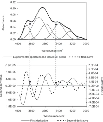
Data analysis started with the analysis of the second and fourth derivatives of the experimental spectrum for overlapped and hidden peaks. Then a resolution enhanced spectrum was obtained according to equation (2). The resolved peaks allowed for initial guesses of the peak maximum ν0 and peak width s. The later was taken as the full width at half height of the resolved peaks. The guess for peak height A was the experimental spectrum value at peak maximum ν0 (Figure 3).
For curve fitting, different models were chosen to investigate the best fit and are presented in Table 1.
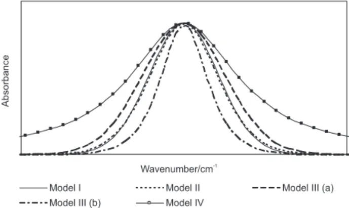
Figure 4 compares the peak shape of each model for a given set of values for ν0, A and s. The Lorentzian fraction of Model II did not alter significantly the overall Gaussian peak shape of that model, as it closely resembles the shape of Model I. The peak shape of Model IV shows the characteristic wide base of a purely Lorentzian peak. Figure 3. Initial guess for peak maximum (νo), peak width s and peak height A.
Figure 4. Peak shapes according to curve fitting models.
Table 1. Curve fitting models
Model Description
Model I – Sum of Gaussian peaks
Model II – Sum of peaks represented by a product of Gaussian and Lorentzian peak with equal peak width
Model III – Sum of peaks represented by a product of Gaussian and Lorentzian peak with different peak width
Model III can assume a variety of shapes, depending on the relative value of the peak widths. If the same value of bandwidth s of the other models is used in the Gaussian part of Model III, a larger value for s’, the bandwidth term of the Lorentzian part, results in a wider peak (Model III (a)) as compared to Model I. A smaller value for s’ results in a narrower peak (Modell III (b)). By proper selection of s and s’ values one can change from a Gaussian like peak shape to a Lorentzian one.
Curve fitting was carried out with the CurveExpert software (available at http://curveexpert.webhop.net/). The goodness-of-fit of the fitted curve and the derivative curves was estimated by the DIS parameter. The analysis was concluded with the comparison of the resolved peaks with those expected from theory, as summarized in Figure 1 and Figure 2.
Results
For the sake of simplification, the curve fitting of the unaged optical fiber only will be given in full detail, with the presentation of the results for all models of Table 1. For the other ageing conditions, only the model with the best goodness-of-fit will be discussed.
Spectrum 1: unaged fiber
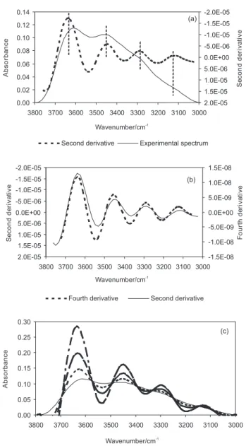
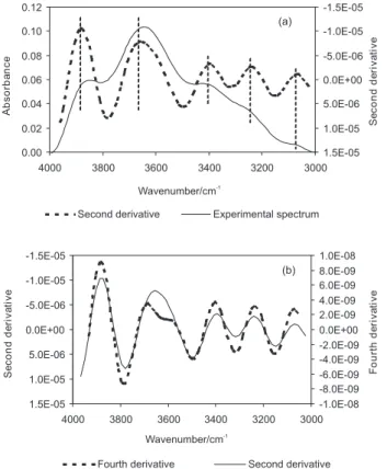
Figure 5a shows the background corrected and smoothed experimental spectrum. Due to the highly overlapped peaks, no single peak or band could be distinguished. Above 3800 cm-1, the spectrum showed no relevant feature and
this part of the spectrum was not considered during further analysis. Superimposed on the spectrum is the graph of the second derivative, which exposed the presence of four peaks at 3640, 3450, 3300 and 3120 cm-1. Higher order
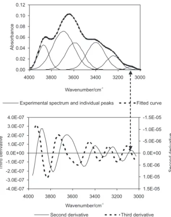
derivatives revealed no additional overlapped or hidden peak, as shown by the graph of the fourth derivative of Figure 5b. A resolution enhanced spectrum could thus be obtained through equation (2) using the second derivative with an appropriate k2 value (Figure 5c), from which initial guesses of the peak maximum ν0, peak height A and peak width s for curve fitting were estimated.
The main findings of curve fitting can be summarized as follows: The different models revealed the same resolved peak pattern, with peaks around 3630, 3475, 3300 and 3125 cm-1 (Figure 6). However, differences were observed
for peak maximum, peak height and peak width (Table 2). The differences for the peak width are understandable, since this parameter is linked to the peak shape. However, it is worth to note that Model III yields two peak width parameters, whose values differ markedly. Since the values
for s, the peak shape parameter of the Gaussian part in the model equation, were closer to the peak width values of the other models, it is assumed that s is more representative of the peak width, whereas the role of s’ is that of a fitting parameter.
Attempts to curve fit with Model IV and to include the peak at 3125 cm-1 proved unsuccessful. As can be seen in
Figure 6d, due to the wide base of the Lorentzian peak, at 3125 cm-1 the total absorbance was made up of the
contribution of the three major peaks at 3630, 3475 and 3300 cm-1. It therefore became difficult for the curve fitting
program to single out a separate peak at 3125 cm-1.
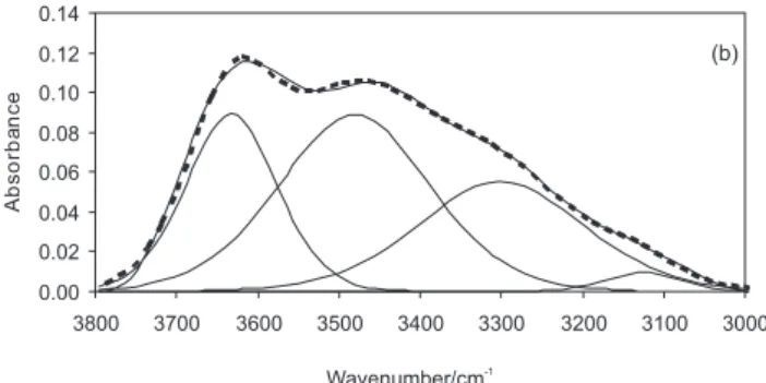
reached with pure Gaussian peak shapes (Model I), which showed the lowest DIS parameter. The worst fit was with Lorentzian peaks (Model IV). This was true not only for the curve fitted spectrum curve, but also for the derivative curves. Moreover, in the composite models (Model II and III), the Gaussian character was predominant in the overall peak shape, as seen in Figure 6b and 6c.
The peak maxima at 3300 and 3125 cm-1 matched closely
the predicted ones from the second derivative curves of the experimental spectrum (Figure 5) and were assigned to the stretching vibrations of free molecular water of Figure 1 (3200-3250 cm-1 and 3140 cm-1, respectively). The peak
at 3475 cm-1 is equivalent to the peak at 3450 cm-1 of the
derivative curve and was assigned to stretching vibrations of adsorbed molecular water 3400-3450 cm-1 in Figure 1. It
is believed that for this peak the shift in peak maximum is a Figure 6. Curve fitting according to the different models. (a) Model I; (b) Model II; (c) Model III and (d) Model IV.
Table 3. Goodness-of-fit analysis – DIS values
Model Fitted curve Second derivative Fourth derivative
I 1.25×10⁻³ 1.58×10⁻⁶ 2.66×10⁻⁹
III 1.38×10⁻³ 1.72×10⁻⁶ 2.85×10⁻⁹
II 1.91×10⁻³ 2.67×10⁻⁶ 4.97×10⁻⁹
IV 7.27×10⁻³ 7.41×10⁻⁶ 1.57×10⁻⁸
Table 2. Numerical results of curve fitting
Initial guess for peak maximum
Parametera Model
I
Model II
Model III
Model IV
3640 cm-1 ν
0 3635.46 3632.36 3633.05 3620.34
A 0.0863 0.0891 0.0885 0.0918
s 79.81 107.02 92.20 58.74
s’ - - 165.86
-3450 cm-1 ν
0 3475.96 3480.75 3471.69 3470.27
A 0.0992 0.0889 0.0982 0.0808
s 138.00 178.21 160.00 101.10
s’ - - 246.50
-3300 cm-1 ν
0 3284.95 3300.35 3286.06 3311.60
A 0.0520 0.0554 0.0506 0.0500
s 121.81 195.40 140.00 109.41
s’ - - 217.85
-3120 cm-1 ν
0 3122.90 3125.25 3127.60
-A 0.0140 0.0096 0.0144
-s 74.40 88.14 92.20
s’ - - 134.59
-aUnit (cm-1), ν
0 - peak maximum, s - peak width and s’ - the bandwidth
result of the curve fitting algorithm. The peak at 3630 cm-1
again matched close the equivalent peak of the derivative curve. It is halfway between the peak ranges of 3595-3625 cm-1 and 3660- 3670 cm-1 of Figure 2 and may be in
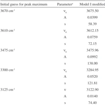
fact an envelope comprising both peaks. To investigate this hypothesis further, an additional curve fitting was carried out. Using Model I, the peak at 3630 cm-1 was replaced
by two peaks with initial guesses at 3610 and 3670 cm-1
and appropriate guesses for peak height and peak width. The result of this curve fit is shown in Figure 7 and in Tables 4 and 5. It can be seen that the peak at 3630 cm-1
can be conveniently substituted by two peaks at 3612 and 3675 cm-1, thus bringing the model closer to theoretical
predictions, since they fall within the 3595-3625 cm-1 and
3660-3670 cm-1 peak ranges of Figure 2. Furthermore, the
splitting up of the 3630 cm-1 peak into two peaks improved
the goodness-of-fit at all levels.
The analysis of this spectrum and its resolved peaks – three below 3500 cm-1 and two above – indicated that
the glass surface of the unaged fiber contained significant amount of both unbounded molecular water and dissolved water (bounded water) in the silica structure.
Spectrum 2: field aged fiber
Figure 8a shows the background corrected and smoothed experimental spectrum. Similar to the previous case, no single peak could be distinguished due to overlapping peaks and no relevant feature was present above 3800 cm-1.
Compared to the previous case, the peak around 3450 cm-1
is more pronounced. The superimposed graph of the second derivative, however, revealed, besides the existence of three well defined peaks at around 3640, 3450 and 3200 cm-1,
the presence of a barely visible peak around 3340 cm-1.
To unveil this peak, it was necessary to further derivate so as to increase the slope differences in the graph, shown in Figure 8b. This time the resolution enhanced spectrum was obtained through equation (2) using the fourth derivative. Curve fitting followed as described for the unaged condition and the main results were as follows: The curve fitted peak maxima matched closely the predicted ones from the derivative curves for all models. The predicted peaks at 3640, 3450, 3340 and 3200 cm-1 varied with curve
fitting in the range of 3619-3640 cm-1, 3453-3468 cm-1,
3320-3353 cm-1 and 3210-3242 cm-1, respectively.
While the 3450 cm-1 is related to adsorbed molecular
water and the 3200 cm-1 peak to free molecular water, the
peak at 3340 cm-1 is a distinctive peak halfway between
both. Although this peak is not related to any type of silica-water interaction described in Figure 1, it is believed that it can be traced to molecular water in silica, too.19
However, this time the goodness-of-fit analysis had to proceed more carefully in order to pick up the most suitable model. Table 6 shows that, from Model I to IV, while the goodness-of-fit of the fitted curve was best for Model I, for the second derivative it was best for Model II and for the fourth derivative it was for Model III. The modified Model I, in which the peak at 3640 cm-1 is replaced by two peaks
with initial guesses at 3610 and 3670 cm-1, improved the
goodness-of-fit in relation to the other models, except for the fourth derivative curve. However, since the goodness-of-Figure 7. Curve fitting with modified Model I.
Table 5. Goodness-of-fit analysis for modified Model I – DIS values
Fitted curve Second derivative Fourth derivative
5.15×10⁻⁴ 9.74×10⁻⁷ 2.51×10⁻⁹
Table 4. Numerical results of curve fitting with modified Model I
Initial guess for peak maximum Parametera Model I modified
3670 cm-1 ν
0 3675.50
A 0.0399
s 58.39
3610 cm-1 ν
0 3612.15
A 0.0759
s 72.15
3475 cm-1 ν
0 3475.96
A 0.0992
s 138.00
3300 cm-1 ν
0 3284.95
A 0.0520
s 121.81
3125 cm-1 ν 3122.90
A 0.0140
s 74.40
aUnit (cm-1), ν
0 - peak maximum and s - peak width, except A. A - peak
fit for the fourth derivative curves of both modified Model I and Model III have the same order of magnitude and are close in value, it was decided to choose the former over the last model. Here again, the splitting of the 3640 cm-1
peak in two smaller peaks at 3622 and 3680 cm-1 (Table 7
and Figure 9) brought the model closer to theoretical predictions.
The resolved spectrum with its predominant peak at 3457.25 cm-1 showed that the environmental conditions
during field exposure (e.g. exposure to high humidity or aqueous environment) had led to water absorption by the silica surface of the optical fiber, despite the protective polymer coating.25 The absorbed water entered the silica
structure as unbounded molecular water. However, under
the prevailing field ageing conditions, the water did show little tendency to react with silica to form bounded water in the form of hydroxyls, despite the long ageing time.
Spectrum 3: 14 days ageing at room temperature and under compressive stress of 0.5 GPa
Figure 10a shows the background corrected and smoothed experimental spectrum. Unlike the other cases, this spectrum showed prominent peaks above 3500 cm-1,
namely at around 3640 and 3900 cm-1. Peaks lower than
3500 cm-1 were hardly distinguishable due to strong overlap.
The analysis of the graph of the second derivative, however, disclosed the presence of three peaks at 3400, 3250 and 3080 cm-1. Moreover, the graph of the fourth derivative of
Figure 8. Resolution enhancement of experimental spectrum. (a) Experimental spectrum and (b) Analysis of derivatives.
Figure 9. Curve fitting with modified Model I.
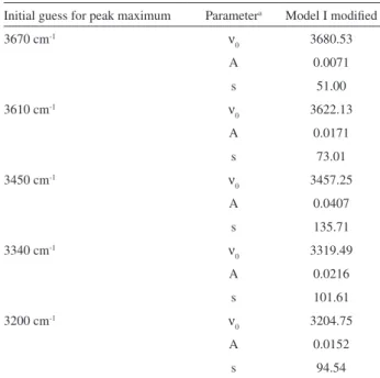
Table 7. Numerical results of curve fitting with modified Model I
Initial guess for peak maximum Parametera Model I modified
3670 cm-1 ν
0 3680.53
A 0.0071
s 51.00
3610 cm-1 ν
0 3622.13
A 0.0171
s 73.01
3450 cm-1 ν
0 3457.25
A 0.0407
s 135.71
3340 cm-1 ν
0 3319.49
A 0.0216
s 101.61
3200 cm-1 ν
0 3204.75
A 0.0152
s 94.54
aUnit (cm-1), ν
0 - peak maximum and s - peak width, except A. A - peak
height.
Table 6. Goodness-of-fit analysis – DIS values
Model Fitted curve Second derivative Fourth derivative
I 3.75×10⁻⁴ 5.51×10⁻⁶ 5.06×10⁻⁹
II 6.09×10⁻⁴ 5.31×10⁻⁶ 3.94×10⁻⁹
III 4.94×10⁻⁴ 5.32×10⁻⁶ 3.90×10⁻⁹
IV 2.47×10⁻³ 6.80×10⁻⁶ 5.68×10⁻⁹
Figure 10b revealed under the envelop of 3640 cm-1 two
hidden peaks, with strong overlapping. The peak maxima were estimated to be around 3700 and 3600 cm-1.
Curve fitting showed that the fitted peak maxima matched closely the predicted ones from the derivative curves for all models. The predicted peaks at 3080, 3250, 3400, 3600, 3700 and 3900 cm-1 varied with curve fitting in the range
of 3080-3087 cm-1, 3241-3260 cm-1, 3397-3400 cm-1,
3580-3600 cm-1, 3660-3700 cm-1 and 3860-3900 cm-1,
respectively. The best fit was again for Model I, with pure Gaussian peaks (Table 8, Table 9 and Figure 11).
From Figure 1 it follows that the peaks at 3080, 3250 and 3400 cm-1 are due to free and adsorbed molecular water,
whereas the ones at 3600 and 3700 cm-1 are due to dissolved
water. The peak at 3900 cm-1 is ascribed to a combination
of various ≡Si−OH vibration modes.2,26
In contrast to the previous cases, where the peak at 3640 cm-1
was artificially replaced by two smaller based on prior knowledge of the system under investigation, in the present case the two peaks at 3600 and 3700 cm-1 showed up in
the derivative curves which were assigned to the 3595- 3625 cm-1 and 3660-3670 cm-1 peak ranges of Figure 1.
Due to the same reason mentioned for Spectrum 1, curve fitting with pure Lorentzian peaks was successful only by excluding the small peak at 3080 cm-1.
The strong presence of peaks associated with bounded water, 3872.51, 3694.04 and 3591.25 cm-1, indicates
that exposure of hydrolyzed silica to compressive stress increased water dissolution into the silica structure as Figure 10. Resolution enhancement of experimental spectrum.
(a) Experimental spectrum and (b) Analysis of derivatives.
Table 9. Numerical results of curve fitting with Model I
Initial guess for peak maximum Parametera Model I modified
3900 cm-1 ν
0 3872.51
A 0.0456
s 70.24
3700 cm-1 ν
0 3694.04
A 0.0710
s 136.61
3600 cm-1 ν
0 3591.25
A 0.0500
s 114.34
3400 cm-1 ν
0 3400.91
A 0.0505
s 115.74
3250 cm-1 ν
0 3241.20
A 0.0257
s 91.96
3080 cm-1 ν
0 3087.60
A 0.0053
s 55.67
aUnit (cm-1), ν
0 - peak maximum and s - peak width, except A. A - peak
height.
Table 8. Goodness-of-fit analysis – DIS values
Model Fitted curve Second derivative Fourth derivative
I 8.72×10⁻⁴ 1.16×10⁻⁶ 2.36×10⁻⁹
II 1.11×10⁻³ 1.27×10⁻⁶ 2.71×10⁻⁹
III 1.20×10⁻³ 1.53×10⁻⁶ 3.34×10⁻⁹
IV 3.69×10⁻³ 4.69×10⁻⁶ 4.37×10⁻⁹
hydroxyl, as expected by theory.27 Dissolution of water in
silica occurs by the following reaction:
H2O + ≡Si−O−Si≡↔≡Si−O−H + H−O−Si≡ (10)
For this reaction to occur, the water molecules have to diffuse into the silica structure to reach propitious reaction sites, e.g., non bridging oxygen atoms, dangling bonds or low angle hydrophilic ≡Si−Ο−Si≡ bonds.28 Tensile stress
favors water diffusion, whereas compressive stress favors dissolution reaction.27
Discussion
For all cases investigated, the combination of the analysis of derivatives with the knowledge of theoretical aspects of the system was important to fully resolve a highly overlapped spectrum. A further aspect to substantiate the analysis carried out herein follows from the application of the peak separation criterion to each pair of overlapping peaks. This will be shown in detail for Spectrum 3, but is easily extended to the other cases.
As stated above, the visual separation of two overlapping peaks by a valley or plateau defines the shoulder limit and is expressed mathematically by equation 8.17 The graphic
representation of this expression is shown in Figure 12 for Spectrum 3. At 3456 cm-1, between the peaks at 3640
Figure 12. The shoulder limit. Top: Location in the spectrum. Bottom: Graphical representation.
and 3400 cm-1,equation 8 is exactly zero and the spectrum
exhibits a valley at the limit of visual perception. If the peak distance gets shorter, the valley would gradually disappear, the minor peak maximum would become less distinctive from the major peak and equation 8 would shift from zero. If the distance gets longer, the valley and the individual peaks would become more discernible and equation 8 would shift from zero again. This last situation is depicted at 3826 cm-1, between the peaks at 3900 and 3640 cm-1. All
other pairs of overlapping peaks are poorly resolved in the original spectrum and equation 8 is far from zero.
Vandengist and De Galan 18 solved equation 8 and
presented the solution in graphical form which shows the shoulder limit of two overlapping peaks for various ratios of peak height (R = A2/A1), peak width (ϕ = s2/s1) and peak distance (δ = [ν2−ν1]⋅[(s2)-1+(s
1)
-1]). Figure 13 shows selected
curves which were retrieved from Figure 1 of the paper of Vandengist and De Galan, which represents graphically the shoulder limit for two overlapping Gaussian peaks.18 The
curves are those with values of R, ϕ and δ closest to the ones of the overlapping peaks of Spectrum 3. The overlapping peaks were placed in Figure 13 using the values of Table 10 which, in turn, were calculated using the values of Table 9. Two overlapping peaks are beyond the shoulder limit and can be visually distinguished if the symbol representing this pair of peaks is above and to the right of the curve with equal ϕ value. Below and to the left, they are under the shoulder limit and cannot be distinguished. For the sake of clarity, a single graph was drawn for each pair of overlapping peak with its respective curves. Hence, in Figure 13a and 13c, the peak at 3872.51 cm-1
can be distinguished from the one at 3694.04 cm-1 and the
peak at 3591.25 cm-1 from that at 3400.91 cm-1, respectively.
However, since the peak at 3694.04 cm-1 cannot be
distinguished from the peak at 3591.25 cm-1 (Figure 13b),
one sees in the experimental spectrum only an envelope comprising both peaks at 3640 cm-1. This larger peak, on
one side, is exactly at the shoulder limit with the peak at 3400 cm-1, since it lies in Figure 13f almost on the curve of
ϕ = 1.7 (between ϕ = 1.6 and ϕ = 1.8), which is the same value of ϕ for the 3640/3400cm-1 pair of overlapping peaks
(Table 10). On the other side, the 3640 cm-1 peak is beyond
the shoulder limit with the one at 3872 cm-1 (Note: To
calculate the values for R, ϕ and δ for the pair of overlapping peaks 3872 /3640 cm-1 and 3640 /3400 cm-1, curve fitting
with Model I was repeated replacing the peaks at 3700and 3600 cm-1 by a single peak at 3640 cm-1). Due to strong
overlapping, the pairs of peaks at 3400.91/3241.20 cm-1
and at 3241.20/3087.60 cm-1 are under the shoulder limit.
Figure 13. Graphical representation of the shoulder limit (curves) and location of the overlapping peaks of Spectrum 3 (symbols). (a) 3872.51/3694.04 cm-1;
(b) 3694.04/3591.25 cm-1; (c) 3591.25/3400.91 cm-1; (d) 3400.91/3241.20 cm-1; (e) 3241.20/3087.60 cm-1 and (f) 3872/3640 cm-1 , 3640/3400 cm-1.
Table 10. Values of R, ϕ and δ for Spectrum 3, as calculated from the data of Table 9
Overlapping peaks/ (cm-1) δ R ϕ
3872.51/3694.04 2.31 0.64 1.9
3694.04/3591.25 0.99 0.70 1.2
3591.25/3400.91 1.99 0.99 1.0
3400.91/3241.20 1.87 0.51 1.3
3241.20/3087.60 2.66 0.21 1.7
It follows from the foregoing that the shoulder limit map of Figure 13 is in close agreement with the spectral features of Figure 12. In fact, this map should be regarded as a validation tool for any peak separation procedure. It not only explains the experimental spectrum obtained, but it also supports the inclusion in curve fitting models of hidden spectral features which are justified from theory.
A similar approach can be adopted for the detection limit, which is defined by an inflection point in the spectrum that coincides with the maximum of the minor peak and is expressed mathematically by equation 9.17 This is
represented graphically in Figure 14 for Spectrum 3. For instance, at 3100 cm-1, equation 9 is nearly fulfilled and the
spectrum shows an inflection point (Figure 15) which is close to the peak maximum at 3087.60 cm-1 (Table 10).
Vandengist and De Galan solved equation 9 and presented the solution again in graphical form.18 Figure 16
Figure 14. The detection limit. Top: Location in the spectrum. Bottom: Graphical representation.
Figure 15. Magnification of the spectrum of Figure 14 at the low wavenumber side.
Figure 16. Graphical representation of the detection limit (curves) and location of the overlapping peaks of Spectrum 3 (filled and open points).
3694.04/3591.25 cm-1; 3400.91/3241.20 cm-1; 3872.51/3694.04 cm-1;
3241.20/3087.60 cm-1; 3640/3400 cm-1; 3872/3640 cm-1 and
3591.25/3400.91 cm-1.
of Spectrum 3. This time, all pairs of overlapping peaks have been plotted in one single graph. To the right of the curves, two overlapping peaks are beyond the detection limit and should be detected with the aid of the second derivative, as was observed for most overlapping peaks of Spectrum 3. To the left, they are under the detection limit and cannot be detected by the second derivative alone. In this case, the presence of overlapped peaks may show up in the fourth derivative or has to be inferred from the previous knowledge about the investigated system. This was the case for the strongly overlapping peaks at
3694.04/3591.25 cm-1, which were perceivable in the
fourth derivative.
The above analysis is in agreement with Figure 10B. In fact, the detection limit map of Figure 16 is an additional tool to the shoulder limit map of Figure 13 to validate a peak separation procedure.
Conclusions
A procedure has been described for reliable peak separation of highly overlapped and hidden peaks in infrared spectra of hydrolyzed silica optical fibers in the 3000 and 4000 cm-1 range. The procedure allowed
for the determination of the number and the locations of the peaks. Through the identified individual peaks it was possible to understand the silica-water interaction processes during ageing of a silica optical fiber. Several points emerged from the analyses that were common to the three examples investigated: (i) In the context of this study, curve fitting with pure Lorentzian peak shape did not prove reliable, since the characteristic wide base of the major peaks excluded the detection of an overlapped small peak and adversely affected the goodness-of-fit; (ii) The best goodness-of-fit, measured by the deviation (DIS) parameter, was obtained with a fitting model using pure Gaussian peak shapes. This was true not only for the fitted spectrum, but also for the second and fourth derivative curve; (iii) Even in the fitting models using compound peak shapes, described by a product of Gaussian and Lorentzian peak shapes, the Gaussian character was predominant in the overall peak shape; (iv) When the silica optical fibers contained more unbound molecular water than dissolved water, the peaks below 3500 cm-1 were predominant and
the peak observed at 3630-3640 cm-1 could be described
of 3595-3625 cm-1 and 3660-3670 cm-1. These two smaller
peaks instead of one larger halfway between both were not evident in the experimental spectrum and its derivative curves, but were closer to theory, i.e., to what is known of the system under investigation. When the fibers contained more dissolved water, however, the peaks below 3500 cm-1
were hardly distinguishable and the peaks in the ranges of 3595-3625 cm-1 and 3660-3670 cm-1 became discernible in
the fourth derivative curve; (v) This study gave a practical example of the utility of the shoulder limit and detection limit maps developed by Vandengist and De Galan.18 They
show the importance to consider hidden and overlapped peaks in a spectrum of the system under investigation that are under the detection limit. These peaks may not be detected even by the fourth derivate, yet their existence should not be excluded. Their inclusion in the fitting model may be justified from theory, i.e., from the existing knowledge of the system, and may improve the goodness-of-fit of the curve fitting.
Supplementary Information
Supplementary data are available free of charge at http:// jbcs.sbq.org.br, as PDF file.
References
1. Lórenz-Fonfría, V. A.; Padrós, E.; Appl. Spectrosc. 2005, 59, 474.
2. Davis, K. M.; Tomozawa, M.; J. Non-Cryst. Solids 1996, 201, 177.
3. Stone, J.; Walrafen, G. E.; J. Chem. Phys. 1982, 76, 1712. 4. http://www.lsbu.ac.uk/water/vibrat.html, accessed in April
2008.
5. h t t p : / / w w w . w a m . u m d . e d u / ~ t o h / s p e c t r u m / IntroToSignalProcessing.pdf, accessed in April 2008. 6. Brereton, R. G.; Chemometrics- Data Analysis for the
Laboratory and Chemical Plant, John Wiley & Sons: Chichester, 2004, 119.
7. Kauppinen, J. K.; Moffatt, D. J.; Mantsch, H. H.; Cameron, D. G.; Anal. Chem. 1981, 53, 1454.
8. Friesen, W. I.; Michaelian, K. H.; Appl. Spectrosc. 1985, 39, 484.
9. Friesen, W. I.; Michaelian, K. H.; Appl. Spectrosc. 1991, 45, 50.
10. Kauppinen, J. K.; Moffatt, D. J.; Hollberg, M. R.; Mantsch, H. H.; Appl. Spectrosc. 1991, 45, 411.
11. Saarinen, P. E.; Appl. Spectrosc. 1997, 51, 188.
12. Lórenz-Fonfría, V. A.; Padrós, E.; Spectrochim. Acta, A 2004, 60, 2703.
13. Moffatt, D. J.; Kauppinen, J. K.; Mantsch, H. H.; Can. J. Chem. 1991, 69, 1781.
14. Holler, F.; Burns, D. H.; Appl. Spectrosc. 1989, 43, 877. 15. Fleissner, G.; Hage, W; Hallbrucker, A.; Mayer, E.; Appl.
Spectrosc. 1996, 50, 1235.
16. Wentzell, P. D.; Brown, C. D. In Encyclopedia of Analytical Chemistry; Meyers, R. A., ed.; John Wiley & Sons: Chichester, 2000, 9764.
17. Maddams, W. F.; Appl. Spectrosc. 1980, 34, 245.
18. Vandegiste, B. G. M.; De Galan, L.; Anal. Chem. 1975, 47, 2124.
19. de Aragão, B. J. G.; PhD Thesis, Universidade Estadual Paulista, Araraquara, Brazil, 2006.
20. Yuce, H. H.; Wei, T.; Estes, R.; Wieczorek, C. J.; Devlin, B. T.; Kilmer, J. P.; Varachi, J. P.; Proceedings 41st International Wire
& Cable Symposium, Reno, USA, 1992.
21. Yuce, H. H.; Proceedings 41st International Wire & Cable
Symposium, Reno, USA, 1992.
22. Frantz, R. A.; Keon, B. J.; Vogel, E. M.; Bowmer, T. N.; Yuce, H. H.; Proceedings 43rd International Wire & Cable Symposium,
Atlanta, USA, 1994.
23. Rondinella, V. V.; Matthewson, M. J.; Proceedings of SPIE 2074, Piscataway, USA, 1994.
24. Tomozawa, M.; Hepburn, R.W.; J. Non-Cryst. Solids 2004, 345, 449.
25. de Aragão, B. J. G.; RTI Redes, Telecom e Instalações 2000, 1, 54.
26. Navarra. G.; Iliopoulos, I.; Militello, V.; Rotolo, S. G.; Leone, M.; J. Non-Cryst. Solids 2005, 351, 1796.
27. Nogami, M.; Tomozawa, M.; J. Am. Ceram. Soc. 1984, 67, 151.
28. Burneau, A.; Lepage, J.; Maurice, G.; J. Non-Cryst. Solids 1997, 217, 1.
Received: May 28, 2008
Web Release Date: October 2, 2008
Supplementary Information
0103 - 5053 $6.00+0.00*e-mail: [email protected], [email protected]
Peak Separation by Derivative Spectroscopy Applied to FTIR Analysis of Hydrolized Silica
Bernardo J. G. de Aragão*,a and Younes Messaddeq b
a Fundação CPqD, Rod. SP 340 Campinas-Mogi Mirim, km 118, 13086-902 Campinas-SP, Brazil
b Instituto de Química, Universidade Estadual Paulista, R. Francisco Degni s/n, 14800-900 Araraquara-SP, Brazil
Table S1. Values of R, ϕ and δ
Overlapping peaks/ (cm-1) δ R ϕ
3635.46/3475.96 a 1.89 0.87 1.7
3475.96/3284.95 a,b 1.75 0.61 1.0
3284.95/3122.90 a,b 2.18 0.25 1.6
3675.50/3612.15 b 1.18 0.53 1.2
3612.15/3475.96 b 1.81 0.79 1.7
a Valid for Model I and bValid for modified Model I.
Supplement 1: Analysis of Spectrum 1
(Unaged fiber)
Shoulder and detection limit maps
From the data of Table 2 and Table 4 of the original paper follows the calculation of the values of R, ϕ and δ, which are given in Table S1.
Figure S1. Shoulder limit.
Figure S1 shows the shoulder limit map for the field aged fibers. The Model I is analyzed from (a) to (c). The 3635.46/3475.96 cm-1 overlapping peaks (a) are just over
the shoulder limit (the limiting line for ϕ = 1.7 lies between
ϕ= 1.6 and ϕ = 1.8), which means that they can still be visually distinguished. All other pairs of overlapping peaks ((b) and (c)) cannot do so, since they are under the shoulder limit. This is confirmed by Figure 4 of the paper.
Using the modified Model I, the peak at 3635.46 cm-1
is substituted by two peaks at 3675.50 and 3612.15 cm-1
which are not visually resolved (Figure S1 (d) and (e)). It is interesting to note that the 3612.15/3475.96 cm-1
overlapping peaks are beyond the detection limit but do not show up in the second derivative. The reason is that the 3612.15 cm-1 peak cannot be detected separately from
Supplement II: Analysis of Spectrum 2
(Field aged fiber)
Curve fitting according to Model I to IV
From Model I to Model III, differences were observed mainly in peak height at 3340 and at 3200 cm-1. Model IV yielded the worst fit (Figure S3). The numerical results are given in Table S2.
Shoulder and detection limit maps
From the data of Table S2 and Table 7 of the original paper follows the calculation of the values of R, ϕ and δ, which are given in Table S3.
Figure S2. Detection limit.
Table S3. Values of R, ϕ and δ
Overlapping peaks (cm-1) δ R ϕ
3641.28/3457.25a 2.24 0.45 1.9
3680.53/3622.16b 1.17 0.42 1.4
3622.13/3457.25b 2.09 0.42 1.9
3457.25/3319.49a,b 1.42 0.53 1.3
3319.49/3204.75a,b 1.41 0.70 1.1
a valid for Model I, b valid for modified Model I.
Table S2. Numerical results of curve fitting
Initial guess for peak maximum Parameter Model I Model II Model III Model IV
3640 cm-1 ν
0 (cm
-1) 3641.28 3637.10 3639.35 3619.23
A 0.0186 0.0185 0.0182 0.0193
s (cm-1) 75.25 101.06 90.00 55.09
s’ (cm-1) - - 132.53
-3450 cm-1 ν
0 (cm
-1) 3456.64 3455.89 3453.11 3468.41
A 0.0416 0.0414 0.0417 0.0330
s (cm-1) 145.52 193.93 173.21 92.07
s’ (cm-1) - - 274.09
-3340 cm-1 ν
0 (cm
-1) 3350.13 3341.63 3320.92 3353.53
A 0.0102 0.0138 0.0164 0.0275
s (cm-1) 83.64 114.48 100.00 75.06
s’ (cm-1) - - 349.82
-3200 cm-1 ν
0 (cm
-1) 3240.04 3231.77 3210.50 3242.51
A 0.0220 0.0198 0.0158 0.0164
s (cm-1) 113.05 142.92 141.42 61.81
s’ (cm-1) - - 117.38
-aUnit (cm-1), ν
0 - peak maximum, s - peak width and s’ - the bandwidth term of the Lorentzian part, except A. A - peak height.
Figure S4. Shoulder limit.
Figure IV shows the shoulder limit map for the field aged fibers. The Model I is analyzed from (a) to (c). The 3641.28/3457.25 cm-1 overlapping peaks (A) are
under but close to the shoulder limit (the limiting line for
peaks at 3457.25/3319.49 cm-1 and 3319.49/3204.75 cm-1
are also under the detection limit (Figure S5). As seen in Figure 7 of the paper, the peak at 3319.49 cm-1 is barely
Figure S5. Detection limit.
Figure S6. Curve fitting results.
visible in the second derivative and its existence is only confirmed by the fourth derivative.
Using the modified Model I, the peak at 3641.28 cm-1
is substituted by two peaks at 3680.53 /3622.13 cm-1
which are not visually resolved (Figure S4 (d) and (e)). It is interesting to note that the 3622.13/3457.25 cm-1
overlapping peaks are beyond the detection limit but do not show up in the second derivative. The reason is that the 3622.13 cm-1 peak cannot be detected separately from
the 3680.53 cm-1 peak, as shown in Figure S5.
Supplement III: Analysis of Spectrum 3
(14 days ageing at room temperature and
under compressive stress of 0.5 GPa)
Curve fitting according to Model I to IV
Table S4. Numerical results of curve fitting
Initial guess for peak maximum Parameter Model I Model II Model III Model IV
3900 cm-1 ν
0 (cm
-1) 3872.51 3869.89 3870.35 3859.98
A 0.0456 0.0457 0.0448 0.0409
s (cm-1) 70.24 95.25 90.00 49.60
s’ (cm-1) - - 109.29
-3700 cm-1 ν
0 (cm
-1) 3694.04 3688.00 3660.73 3690.22
A 0.0710 0.0695 0.0901 0.0612
s (cm-1) 136.61 184.45 181.66 92.45
s’ (cm-1) - - 250.51
-3600 cm-1 ν
0 (cm
-1) 3591.25 3590.32 3579.78 3595.42
A 0.0500 0.0485 0.0183 0.0572
s (cm-1) 114.34 165.22 164.32 93.59
s’ (cm-1) - - 168.69
-3400 cm-1 ν
0 (cm
-1) 3400.91 3400.17 3398.63 3396.76
A 0.0505 0.0449 0.0443 0.0377
s (cm-1) 115.74 151.10 148.32 95.94
s’ (cm-1) - - 151.98
-3250 cm-1 ν
0 (cm
-1) 3241.20 3248.77 3248.35 3260.80
A 0.0257 0.0262 0.0263 0.0184
s (cm-1) 91.96 138.13 137.84 56.73
s’ (cm-1) - - 135.25
-3080 cm-1 ν
0 (cm
-1) 3087.60 3080.93 3081.64
-A 0.0053 0.0041 0.0041
-s (cm-1) 55.67 64.89 64.81
-s’ (cm-1) - - 70.28
-aUnit (cm-1), ν