Determination and forecast of agricultural land prices
Bastiaan Philip Reydon* Ludwig Einstein Agurto Plata** Gerd Sparovek***
Rafael Guilherme Burstein Goldszmidt**** Tiago Santos Telles*****
Abstract
he aim of this study is to discuss and apply he-donic methodology for the determination and forecast of land prices in speciic markets. his is important due to the fact that there is no oicial or reliable information in Brazil on current prices in land market transactions. his hedonic price methodology uses a multiple regression model which has, as an explanatory variable, the price per hectare and independent variables related to physical attributes (soil, climate and terrain), pro-duction (systems of propro-duction, location, access), infrastructure of the property and expectations (regional scenario, local investments). Applica-tion of the methodology to a Homogeneous Zone of the state of Maranhão, in Brazil, generated a parsimonious model, in which ive independent variables were responsible for % of the variance in the price of agricultural land.
Resumo
O objetivo do presente trabalho foi discutir e aplicar a metodologia de preços hedônicos para determinação e previsão do preço da terra rural em mercados especíicos. A sua importância decorre do fato de que
não existem no Brasil informações oiciais ou idedignas sobre preços praticados nos negócios com imóveis rurais. Essa metodologia de preços hedônicos utiliza um modelo econométrico de regressão múltipla, tendo como variável dependente o preço por hectare, e como variáveis explicativas as relacionadas ao meio físico (solo, clima e relevo), à produção (sistemas de produção, localização, acesso), à infraestrutura do imóvel e às expectativas (situação regional, investimentos locais). A aplicação de tal metodologia a uma zona homogênea do Estado do Maranhão implicou um modelo parcimonioso, em que cinco variáveis independentes permitiram a explicação de % da variância do preço por hectare da terra rural.
Keywords
land market, hedonic prices, multiple regression analysis, land policy
JEL Classification
R14, R15
Palavras-chave
mercado de terras, preços hedônicos, análise de regressão múltipla, política fundiária
Classificação JEL
R14, R15
*Professor Livre Docente IE/UNICAMP
**Professor Pleno FATEC
***Professor Titular ESALQ/USP
****Professor Adjunto EBAPE/FGV
1_Introduction
In Brazil, prior to the economic stabilization of , the issue of determination of agricultural land prices was frequently relegated to the sidelines for two reasons: irstly, it was considered to be a preoccupation only of landowners and secondly, due to the diiculties in calculation on account of the high inlation. However, the result of Brazilian land policies and disputes in the courts, amongst other issues, have been demonstrating the importance that the determination and forecasting of adequate rural and urban land prices exerts in Brazil today.
Land market dynamics and the consequences of the evolution of its prices have played a crucial role in the aims and goals of land policies and land administration. For instance, the sharp reduction in agricultural land prices, following the Plano Real in , signiicantly favored the attainment of the goals for land reform in the irst term of President Fernando Henrique Cardoso (Delgado, ; Sallum Junior, ). Along with the democratization of land through the market, which began in , the programs Cédula da Terra (Land Bill),
Banco da Terra (Land Bank) and Crédito Fundiário (Land Credit) had, because of acquaintance with the markets and construction of suitable policies, many diferent impacts. While the Cédula da Terra, because of subsidies ofered with these agreements made at lower than market price, reduced market prices, the Banco da Terra, without subsidies and without price supervision, expanded the demand for land, thus signiicantly increasing its price (Reydon and Plata, ).
In various legal skirmishes, the expropriation of land for land reform and land purchases for the programs called “access to land through the market” have been concluded using market prices. But how is market price
established? How to unravel the variables that determine the dynamics of the land price in a speciic geographical location or local market? What kind of model should be used to forecast this price? his article contributes with a methodology for forecasting the land price in speciic markets with the aim of providing supporting data, amongst other aims, to the agricultural policymakers in charge of democratizing access to rural land in Brazil.
In the specialized international literature on agricultural economics, empirical papers like those of Peters (), Lloyd, Rayner and Orme (), Lloyd () and Hallan, Machado and Rapsomanikis (), concentrate their explanation of agricultural land price dynamics from a macroeconomic perspective. hese authors recognize that agricultural land is an asset and that its price is determined by the capitalization of future income obtained from its productive and speculative use. Productive incomes are derived from agricultural products while speculative incomes derive from their characteristic as an asset that maintains value over time. In the case of Brazil, because of the experience of high inlation, speculative use has had a large impact as shown by studies like those of Pinheiro (),
Reydon (), Brandão () Brandão and Rezende (), Bacha (), Reydon (), Reydon and Romeiro () and Plata ().
2._Theoretical parameters
2.1_Hedonic price
Hedonic price analysis is a statistical technique
developed more than seventy years ago to assess product quality issues. here are two basic approaches in the literature to understanding price characteristics.
One tradition relates this price to a consumer’s willingness to pay for a characteristic. his utility-based interpretation is relected in the use of the term hedonic to describe the approach, and was the original view of the subject matter adopted by Andrew Court (Goodman, ) and other early practitioners. Lancaster () proposed a theory of consumer utility based on characteristics rather than on goods, thus it is possible to establish a relationship between the value of the goods and their characteristics. From this, Lancaster proposed the existence of two stages in the relationship between individuals, goods and their characteristics: one between goods and their characteristics (technical relationship) and the other between individuals and the characteristics of the goods (individual preference relationship). Pendleton and Mendelsohn () described the rather restrictive conditions under which the hedonic function can be derived from an underlying utility function.
On the other hand, the second approach, developed by Rosen (), has generally been accepted as the paradigm of the hedonic approach. Rosen relates the hedonic function to the supply and demand for the individual characteristics of each commodity. he hedonic approach is a method that estimates a function that relates the price of the commodities to the diferent attributes that it possesses (implicit price).
Rosen () based his argument on two pillars: irstly the fact that the product has a price and secondly that it has
measurable characteristics or attributes which deine the so-called hedonic price or implicit price. Rosen () also assumes that consumers purchase one single unit of the asset with its particular characteristics. As the author states, additions in income always increase maximum utility and therefore it should be expected that consumers with higher incomes will purchase larger quantities of characteristics. However, in general, there is no reason why the quantities required for all features must always increase with income, since some of their components may increase and others decrease. Consequently therefore, the model has a natural market segmentation, where consumers acquire cash to buy similar products with similar characteristics.
According to this theory, a class of goods that are described by their n attributes or characteristics deines the competitive market. he components of this vector are thus measured as each consumer assesses each characteristic equally. However, there are diferences in the valuation of each ‘features package’ for each agent market. Each product has a share of the market price and is associated with a ixed value of the vector q, revealing an implicit function p (q) = p (q, q, ..., qn) relating prices and characteristics. his function is equivalent to hedonic regression rates obtained by comparing search rates with diferent characteristics.
his view was explored further by many authors, including Triplett (), Epple (), Feenstra () and Pakes (). he methodology has recently been used extensively in real estate, with Plantinga and Miller (), Bastian et al. (), Angelo et al.(), Taylor and Brester (), Arraes and Souza Filho (), Guiling et al. (), Kostov (), Sander and Polasky (), Deaton and Vyn (), Ma and Swinton () and Jaeger et al. ().
2.2_Agricultural land price determination
he price of agricultural land, in a speciic geographical area, relects the existing market structure and the political and socioeconomic development of the region. Market prices guide the private economic agents in the land market in purchases and sales; they are also a reference for the government in its rural democratization of access to land and in land taxation programs; they are used by credit institutions for the computation of the mortgage and land valuation as a guarantee for rural loans. Consequently the price of land is, on the one hand, the relevant variable that expresses the expectations of the economic agents for this resource and, on the other hand, it acts as a signal to be considered by the policy makers when it is proposed to deine eicient economic and social land use and distribution.
But how to estimate and describe the dynamics of prices in imperfect land markets, as is the case in Brazil, in which land has a ixed, immovable and concentrated supply? On the one hand, land can be used as a productive factor in the production of rural goods and, on the other, as a speculative asset, as it maintains value from one period to another. here are also rules concerning its usage (for instance, the legal forest reserve) and taxes on properties, besides the cultural and socio-political characteristics that afect the market. In
this context, the rural land price synthesizes the efect of all the factors that interact in its market. herefore, this paper discusses, in theoretical and empirical ways, the determinant variables for land prices and the dynamics of the land market in Brazil.
heoretically, it is assumed that these land markets are established in capitalist economies in which the economic agents have expectations and make decisions to obtain maximum monetary gain. In this scenario, of
enterprise and market economies, the owners of wealth obtain diferent kinds of assets, with diferent levels
of liquidity to obtain monetary gains and protection from the uncertainties of the capitalist economy and try to predict the psychology of the markets and decide whether or not to buy the assets that, according to their expectations, will provide higher net returns (Reydon, ; Plata, ; Reydon and Plata, ).
Rural land is an important asset because it possesses three particular characteristics: (i) scarcity; (ii) physically immobility; and (iii) durability (Dasso et al., ). he scarcity of land is not only a consequence of its physical scarceness, but also the scarcity of the products that emanate from it. However, being an immobile factor that cannot be reproduced, the economic scarcity of land is caused by its low elasticity of production and substitution, which can be privately appropriated by some agents. Nevertheless, the development of technologies that increase its productivity, as well as administrative measures such as land reform, for example, can substantially modify the level of land scarcity in a region (Plata, ).
with any changes in legislation or in the guarantees that a property may have, its condition as an asset
becomes more uncertain, increasing the risk associated with acquisition and decreasing the liquidity, rate of capitalization and its price (Deininger and Feder, ). he reference assumed here has always been the property,
irrespective of its form, because in some areas or countries, where the property is not formally established but socially accepted and land is traded, there is a land market (Binswanger et al., ).
Land prices are the result of a trade between purchasers and sellers in the land markets, but this trade only occurs when a purchaser has higher expectations than the seller about the future gains from that land. Consequently, the changing expectations of future gains from the land and, therefore, its price, are the most important variables in understanding the dynamics of the land market (Case and Quigley, ).
In summary, rural land can be characterized as being, simultaneously, a capital and a liquid asset, negotiated at lexible prices – established by the capacity of the owners to accumulate the asset. he main reason for this is that the supply of land is ixed and the market price will be
determined by the dynamics of demand.
he expectations of the owners can determine the quantity of land to be negotiated, but the purchasers’ expectations of future gains with the use of the land is what will establish the price. In this context, according to Reydon (), similar to all assets, the price of rural land is an expression of the prospective gains for the three capitalized attributes:
P = q – c + l
Where:
q – productive quasi-rents: the expected gains from productive uses of the property. he value of this attribute depends on the expected gains from rural production and the possibility of other gains resulting from possession of the land, such as credits or government subsidies.
c – maintenance costs: expected costs of maintaining the land in the portfolio of the agent; this means all the non-productive costs associated with the property, such as the transaction costs, land taxes and the like.
l – liquidity premium: the ability to sell the land in the future. his is the least objective part of the price computation and is primarily formed by the agents’ expectations in relation to the land markets. It is higher when the economy grows and the demand for land as a capital asset increases, or when there is an increase in the demand for liquid assets. Sometimes, in a crisis, when expectations for other liquid assets are worse than they are for land, its liquidity may also grow.
It is important to emphasize that the speciic, local Brazilian land markets are imperfect mainly because: a) of a signiicant political and social inequality of property distribution; b) an individual economic agent can manipulate the supply and the price of land; c) the landless need land but they are economically unable to obtain it; d) land is not a simple product, the properties have diferent dimensions, quality, fertility and surfaces; e) there are spatial conditions that afect the price (Plata, ; Reydon, ). Empirical evidence shows, however, that regions with dynamic land markets also have dynamic product, labor and credit markets (Case and Quigley, ; Alston et al., ; Lambin et al., ; Barbieri and Bilsborrow, ).
It is important to emphasize that land markets have two diferent segments: the trade market and the rental market. On the one hand, an economic agent that operates in the trade market is willing to pay for the total possible gains: the productive quasi-rents and the liquidity premium of the land. On the other hand, renters will be willing to pay a rent based just on
productive proit and, because of this, the value of the rent of the land can be considered as a proxy variable of its productive gains.
2.3_Variables in land price determination
Based on the aforementioned theory, it can be stated that the land price in a speciic market is determined by the expected productive and speculative gains from the property. he main variables that explain the dynamics of these gains and the land prices are:
• he overall demand and prices for products from speciic farming activities. his demand is determined by prices of products and by input costs such as: technology, mechanization (capital) and other factors used in production. In microeconomic terms, the productive proit from land use at a particular moment in time would be similar to the expected value of the land’s marginal product. So, the productive gain from land would
depend on the market conditions for the product and the technical conditions for production, because the land’s marginal physical productivity is a consequence of a technical relationship with other factors in a speciic technology. An increase in the price of the product, due to an increase in proit or a change in consumer preferences, creates expectations of an increase in productive proit.
he same occurs when production costs fall (in the case, for instance, of a decrease in the price of assets, ease of access to capital, improvement in technology and/or in the conditions of production), which increases the production function and the physical productivity of the land.
• he large increase in land use for food and energy production around the world in the last ten years has had a big impact on demand and the price of land in all developing countries, particularly in Latin America and Africa (Cotula, and ; Msangi and Ewing, ; Deininger, ).
• he infrastructure of production and trade afects the expected productive gains from land. he existence of irrigation infrastructure, availability of water, access, transportation, proximity to the centers of consumption and information has a positive efect on land prices, as well as decreasing the risks to its productive gains. In many cases, these variables determine the diferent land prices locally.
• Institutional restrictions on the utilization of land create negative expectations about productive gains, decreasing the price of the land. Good examples are the Laws of Forestry Preservation (Forest Code) that reduce land prices. On the other hand, the social beneits from the preservation of the environment can be high and the alternative use of rural land, such as ecological tourism, can generate optimistic expectations of increased gains from land.
land, the impact of fragmentation on land prices depends on the area required for
eicient agricultural exploration in the region (Reydon et al., ).
• Population growth can have an important efect on land prices for at least two diferent reasons: an increase in demand for farming products (food) and space for urbanization and leisure. he increase in demand for land for non-farming purposes mostly increases prices only with a Homogeneous Zone.
• Inlation afects land prices in two ways: irstly, by changing productive gains, due to the increase in the price of products and inputs. he second and
more important way relates to land’s capacity to retain value derived from its liquidity. So there is a potential demand for land that will be determined by the expectation of gains in contrast to other real and inancial assets. For instance, in , during the Plano Real when inlation was defeated, land prices fell about % in real terms (Plata ; Reydon et al, )
• he demand for land in inlationary contexts is strongly related to the efect of inlation on real interest rates. If real interest rates are negative, inancial assets are not attractive and, therefore, the investors will look elsewhere for real assets, such as real estate, houses, urban areas, agricultural land etc. (Reydon and Plata, ).
• Rural land taxes can afect price insofar as they raise the cost of maintenance. A land tax has the virtue of encouraging an increase in the productivity of idle land or where there is a low level of utilization (Reydon and Plata, ).
• he level of development of a country’s inancial system afects the price of rural land. he absence of liquidity in an economy is important because it increases the opportunity cost of money. In the case of agricultural business, with long-term investments, liquidity constraints are frequent. For example, in a country with an underdeveloped inancial system, only those agents that have portfolios with highly liquid assets can purchase
land. As a consequence, there will be little demand for the purchase of land, but the demand to rent land will be higher.
• Transaction costs in the land markets are the combination of several costs: bureaucracy, research, asset evaluation, management costs etc. High transaction costs in the land market are the major factor behind the low incentive to trade in land. • Finally, the socioeconomic and political
3_Methodology for rural land price determination
in specific markets
10his item presents a methodology for determining rural land prices in speciic markets in Brazil, deined as Homogeneous Zones. he Homogeneous Zones are deined by cluster analysis, using Ward’s method (Ward, ) and SPSS sotware, based on the similarity of municipalities with regard to a set of characteristics: the land’s agronomic condition, location, the main stakeholders in the market, level of mobility, expected purchase prices and level of urban development.
Land prices in speciic markets are determined by local variables, so markets have to be analyzed using disaggregated information. To use the state or province level in Brazil would be too aggregated, so these will be divided into Homogeneous Zones, aggregating municipalities using cluster techniques. he variables used to aggregate the municipalities in order to form the Homogeneous Zone are primarily economic, social and agronomic. Ater the aggregation of municipalities into Homogeneous Zones, a questionnaire will be applied for each state to a random sample of recently traded properties, to capture values for the main variables which will be taken into account in the forecast land price model.
he methodology used to study rural land prices in speciic or local markets observes the following stages: i) formation of a secondary database to establish Homogeneous Zones through cluster techniques, using secondary information, ii) formation of a primary database with the application of a questionnaire to the purchasers of rural properties, by stratiied samples, to ind real land prices and the explanatory variables, iii) statistical analysis of the primary information database to exclude incomplete or incorrect data, such as extreme values, and to obtain responses focusing on the market price equation,
and iv) create a computer program (oline) and build a database (web) to estimate land prices from information obtained from people accessing the system.
3.1_Primary information from a Homogeneous Zone (fieldwork)
he primary information for the study of land price dynamics in speciic markets will be obtained through ieldwork conducted using random sampling of properties traded in a Homogeneous Zone. he sample must be distributed proportionally to the number of municipalities that make up the Homogeneous Zone. he sample has to achieve a minimum of deals per Homogeneous Zone.
he cadaster of trades by municipality, used to deine the random sample, consists of a list of completed deals for the respective areas, obtained from the public notary. During interviews, the researchers use printed application forms that are illed out and they get electronic codes. Another program receives the database which is analyzed and the inal processing is performed. hese stages are as follows: more advanced critical
routines with registers being checked for duplication, extreme values, as well as several other logical processes like: price delation, composition of data and interaction with the external database. he outcome at this stage is a database which will be used for the statistical analysis.
questionnaire that generated more than variables. he variables cover the following types of property
characteristics: physical (soil, climate, topography), productive (system of production, location, access), infrastructure of the property (fences, buildings) and expectations (regional situation, local investments). his information was input to the database to be used in the statistical analysis that deined equations for the land price determination.
3.2_Model to determine the land price in a Homogenous Zone
From the reined database, using as a minimum unit of analysis the deals completed in a Homogeneous Zone, consisting of a group of municipalities, multiple regressions were estimated to establish equations to determine land prices to be used as a basis for the forecasting of the price for a speciic property. he model uses, as a dependent variable, the rural land price at a speciic moment in time and, as independent variables, the farms’ relevant characteristics that explain the land price in the same speciic market. he estimation method is that of the ordinary least squares (OLS), with the use of the forward stepwise technique. his technique consists of the inclusion of the variables of highest explanatory power in the regression equation, which in statistical and theoretical terms, contribute to a higher level of explanation of the variation of the dependent variable. he stepwise technique permits a more parsimonious
model to be attained, which will be used to predict prices while observing, however, the theoretical relationship between dependent and independent variables.
Land prices are determined by two types of variables: productive, those related to land as a
production factor and speculative, those related to land as an asset that maintains value. To study the variable
efects on land prices in speciic markets, from the information collected in the ieldwork, the following equations will be estimated:
PRICEt = a + aXt + aXt + .... + akXkt I = , ,...k t = ,,...n
PRICE: Price per hectare of property negotiated. his variable can be represented by the current price (PCTE) or by the real market price (PREAL). he latter was obtained using the current price delated by the IGP-DI general price inlation index, base January .
Xi: represents the relevant variables that explain the variation in rural land prices in the speciic market. hese variables can change from one Homogeneous Zone to another.
t: represents the diferent Homogeneous Zones.
he basic hypothesis which it is aimed to test in the model () is the existence of a signiicant relationship between the speciic market and the proxy variables that capture the expectations of the buyers at the time of deciding the land price.
3.3_Updating of the model of land price determination
Whenever new property trades have been analyzed, they can be included in the sample. It will permit an improvement of the equation due to there being a larger sample. In the case of the Land Credit Program, the loan obtained to purchase the land will permit a quick improvement in the sample, making it easier to update the model. his updating will be achieved by inserting the same variable in all the new deals from the government programs: Consolidação da Agricultura
Familiar (Consolidation of Family Farming – CAF),
Crédito Fundiário de Combate a Pobreza Rural (Land Credit and Poverty Alleviation Program – CF-CPR) and Nossa Primeira Terra (Our First Land – NPT). he addition of data will be performed through the integration of the collected program and analysis of data used in the routine PNCF (National Land Credit Program) process linked to a database on the web, which receives and stores the new information. his model update process requires a model maintenance team which will monitor data input and make the necessary adjustments to the equations, so that they relect market changes and incorporate the new data.
4_Application to the state of Maranhão, Brazil
his item presents the application of the hedonic land price model to the case of a Homogeneous Zone in the state of Maranhão, in northeastern Brazil. Using cluster analysis, it was possible to identify four major Homogeneous Zones, as illustrated in Figure . From the four Zones, the Homogeneous Zone chosen was number (in red in Figure ), with municipalities. From these municipalities, for the ieldwork, questionnaires were collected in sampled municipalities.
4.1_Refinement of the sample
In Homogeneous Zone , despite the strict control over the data collection process, the possibility of incorrect values had to be carefully considered. Very low or very high prices could be an indication of some kind of problem with the data. hus, the reinement of the sample was based on the upper price limit with a % conidence interval. Due to the high dispersion of prices, the lower limit of the conidence interval was
negative. Transactions with prices under R$ . per hectare were eliminated based on a qualitative analysis of the market which indicated that such values would be extremely atypical. One observation showed a price under R$ . per hectare, and the prices in six cases were higher than the upper limit of the conidence interval (R$ . per hectare).
Synthesizing the observations, according to the sample the average land price is R$ ., with a minimum value of R$ . and a maximum of R$ .
Figure 1_Geographic distribution in Homogeneous Zone in the state of Maranhão, Brazil.
Source: Author, based on ield survey data.
211
212
213
and a standard deviation of R$ .. Seven cases were eliminated as outliers detected via Mahalanobis Distance, Cook Distance or Standardized residuals, leaving observations in the inal model.
4.2_Multiple regression model and model variables
he multiple regression model, used to explain and forecast the land price in Homogeneous Zone , starting
from a group of about variables using the forward stepwise technique, selected explanatory variables. he
logarithm of land price per hectare (LNR$/ha) was the dependent variable.
he variables that best explained the land price are those described in Table .
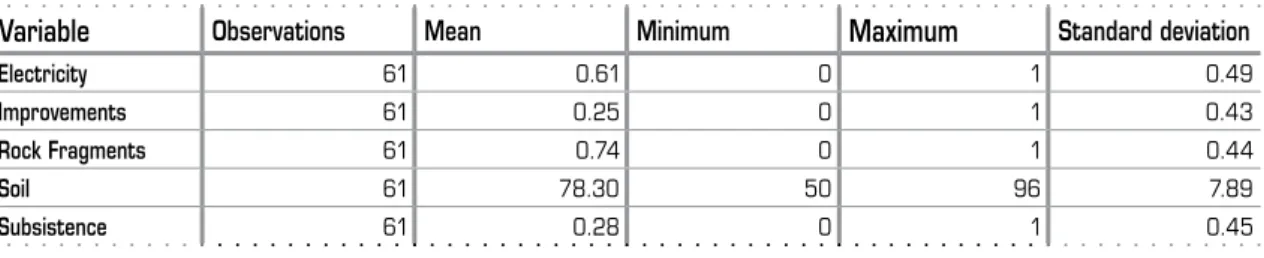
Table presents descriptive statistics of the independent variables.
Variable Description Expected sign of the estimated coefficient
Electricity Dummy variable that indicates access to electricity. It has a value of 1 when the farm has access to electricity, otherwise 0.
Positive, as besides representing benefits from electricity itself, this variable may be a proxy of other characteristics of infrastructure, which usually come together with electricity.
Improvements
Dummy variable that indicates the existence of improvements on the farm, such as barns, for example. It has a value of 1 if there are improvements on the farm, otherwise 0.
Positive, since improvements increase production options.
Rock Fragments
Dummy variable that indicates the presence of rock fragments, which is considered to be good (1): soil with no mechanization restrictions due to rocks, or bad (0): soil with rock fragments that makes mechanization impossible.
Positive, since it is expected that the property, where rocks do not interfere with the use of mechanization, have higher prices. Those in which rock fragments make mechanization impossible have lower prices.
Soil Composite index that considers soil’s physical properties, such as depth and texture. This index varies in a range from 10 to 100.
Positive, as soil with better physical properties permits greater land productivity and rent.
Subsistence
Dummy variable; value 1 when the system of production of the property is agriculture and cattle-raising related to subsistence and trade of surplus, and 0 in the opposite situation.
The sign depends on the group of production systems in the Homogeneous Zone in question.
Table 1_Description of model variables.
Source: Author’s elaboration based on ield survey data.
Table 2. Summary statistics of independent variables
Variable Observations Mean Minimum Maximum Standard deviation
Electricity 61 0.61 0 1 0.49
Improvements 61 0.25 0 1 0.43
Rock Fragments 61 0.74 0 1 0.44
Soil 61 78.30 50 96 7.89
Subsistence 61 0.28 0 1 0.45
he mean, in the case of dummy variables, represents the fraction of cases in which the variable assumes the number as value (e.g. % of the cases have access to Electricity).
4.3_Estimated coefficient
he regression model explains approximately % of the variance of the natural logarithm of land price per hectare, as can be seen in Table . Table also shows the main statistics from the econometric model to predict the natural logarithm of the price of rural land per hectare in Homogeneous Zone .
Table presents the value, standard error, statistic t and p-Value of the estimated coeicients.
Table 3_The estimation results.
Intercept/Variables Value Standard
error Statistic t p-Value
Intercept 2.831 0.434 6.531 0.000
Electricity 0.293 0.085 3.442 0.001
Improvements 0.455 0.092 4.943 0.000 Rock fragments 0.450 0.104 4.317 0.000
Soil 0.019 0.006 3.292 0.002
Subsistence -0.254 0.089 -2.852 0.006
R2 0.70
R2 adjusted 0.68
F statistic 26.17
Source: Author’s elaboration.
According to Table , all the variables were signiicant to an error level lower than %. All the coeicients present the correct sign, as deined in Table .
he regression intercept indicates that, when the valueof all thedependent variables is zero, the price forecast by the model is R$. per ha (antilog of
.). Because the dependent variable is the natural logarithm of rural land area, the value of B has diferent interpretations, which varies according to the functional forms of the explanatory variable referred to, such as described in Table
Table 4_Interpretation of parameters of the variables.
Explanatory variables coefficient
(functional form)
Interpretation of estimated coefficient
Continuous variable
Logarithm of the rate of variation – the fo-recast value is multiplied by eb for each
unit change in the explanatory variable.
Dummy variable
Logarithm of the price variation factor – the forecast value is multiplied by eb when
this variable equals 1.
Source: Author’s work on Gujarati ().
he B coeicient of the dummy variable Rock Fragments (.) indicates that, when they do not interfere with the mechanization of the land, the forecast price of the property is multiplied by factor e., or that it
increases by .%.
he B coeicient of the dummy variable Improvements (.) indicates that, when there are adequate improvements, the forecast price of the property is multiplied by the factor e., or that it
increases by .%.
he B coeicient of the dummy variable Subsistence (-.) indicates that, when the property is used mainly for subsistence purposes, the predicted price is multiplied by the factor e-., or that it is reduced by .%.
he B coeicient of the Soil variable (.) indicates that an increase of one point in the soil index raises the predicted price of the property by .%.
4.4 _Assumptions of the linear regression model
Linear regression model estimators by OLS are BLUE (Best Linear Unbiased Estimator) when the residuals are homoscedastic and normally distributed. Moreover, to interpret consistently the estimated parameter sign and magnitude, no serious multicollinearity problems must be present.
Multicollinearity is an econometric problem diicult to avoid when working with cross-sectional data (data at a point in time, which show a global overview) and many explanatory variables. his study of determination of land price possesses these characteristics. Several practical rules have been developed to determine which way the problem afects the estimation of the model and which variable or variables cause it. Multicollinearity makes reference to the existence of linear relations between the explanatory variables in the model. he variance inlation factor (VIF) is the most frequently used indicator in its identiication. VIF valuesover are taken as a sign of severe problems.
In Table , the column Tolerance indicates the converse value of the inlation factor variance and thereforetolerance values below . indicate problems of multicollinearity.he tolerance is equal to - R-square, in which R-square is the coeicient of determination of the regression in which the explanatory variables in question are taken as a dependent variable and the other explanatory variables as independent variables in the new model.
As indicated in the table above, the Tolerance value for all the explanatory variables of the models is above ., which indicates the absence of serious problems of multicollinearity.
Another relevant assumption of the multiple regression analysisis the normality of theresiduals. he term of error of this regression model represents the aggregate efectof several variables related to the land price, which were not included as explanatory variables. hrough the Central Limit heorem, the joint distribution of such variables is normal. A bias from normality could indicate an error of speciication, which means a relevant variable not included in the model. Moreover, the hypothesis tests of the linear regression model using OLS arebased on a normal distribution of residuals.
Table 5_Multicollinearity indicators.
Variable Beta Partial correlation
Semi partial
correlation Tolerance R-square Statistic t p-Value
Electricity 0.27 0.42 0.25 0.87 0.13 3.44 0.001
Improvement 0.37 0.55 0.36 0.96 0.04 4.94 0.000
Rock fragments 0.37 0.50 0.32 0.72 0.28 4.32 0.000
Soil 0.28 0.41 0.24 0.76 0.24 3.29 0.002
Subsistence -0.22 -0.36 -0.21 0.94 0.06 -2.85 0.006
he results of the regression indicated that the null hypothesis of residual normality in the Kolmogorov-Smirnov test could not be rejected with a signiicance level lower than %. his means residuals can be considered normal (Table ).
Heteroscedasticity occurs when, contrary to homoscedasticity, the term of error variance is not constant, a situation in which estimates via OLS are no longer eicient. One of the tests of heteroscedasticity most frequently used is the White test in which a regressionis estimated where the dependent variable consists of the residualsand the independent variables are as per the original model; their squares and their cross products are the dependent variables. Under the null hypothesis of homoscedasticity,the size of the sample (n) multiplied by R of the auxiliary regression,
follows a distribution c with degrees of freedom equal to the number of regressors, i.e. n R ~ c gl. A value of this statistic, above the critical value cto a particular signiicance level, indicates problems of heteroscedasticity (Gujarati, ).
he regression of residualswiththe independent variables of the original model, its square andcross product results indicated that:
(i) the p-Value associated with statistic c (. – squares) does notlead to a rejection of the null hypothesis with a signiicance level lower than %, which indicates the absence of heteroscedasticity (Table ); and
(ii) the p-Value associated with the statistic c (. – squares and cross products) does not lead to rejection of the null hypothesis with signiicance lower than %, which indicates the absence of heteroscedasticity problems (Table )
Moreover, the values predicted by the model and the real valuesof the property, in the order of the latter,
Table 7_Testing homoscedasticity of the residuals (squares of the residues)
Source: Author’s elaboration.
Intercept/Variables Value Statistic t
Intercept -0.4087 -0.6812
Improvements -0.01496 -0.5392
Soil 0.0121 0.7714
Electricity -0.01402 -0.5414
Rock fragments 0.000613 0.01951
Subsistence -0.001462 -0.05431
Soil² -7.168e-005 -0.6972
Residual sum of squares 0.400508
Sigma 0.091345
c² (6) 2.4009 (0.8794)
F statistic (6.48) 0.32778 (0.9191) Table 6_Residual Kolmogorov-Smirnov normality test
Results Mean Standard
deviation Absolute Positive Negative
Normal
Parameters (a, b) 0.00 0.29 - -
-Most Extreme
Differences - - 0.12 0.08 -0.12
N 61.00
Kolmogorov-
Smirnov Z 0.90
p-Value 0.39
demonstrate the adequate adjustment of the model with all forecasts lying on a % conidence interval (Figure ). Finally, it is important to stress that this model can only be used for forecasting purposes for the range of valuesof the dependent variable of the database from which it was estimated.
Table 8_Testing homoscedasticity of the residuals (squares of the residues and cross products)
Variable/Intercept Value Statistic t
Intercept -1.059 -1.049
Improvements -0.1362 -0.2981
Soil 0.02595 0.9657
Electricity 0.4808 1.144
Rock fragments -0.0595 -0.1008
Subsistence -0.2996 -0.8923
Soil² 0.0001379 -0.7284
Soil*Improvements 0.001312 0.2217
Electricity*Improvements -0.02316 -0.3231
Electricity*Soil -0.007114 -1.287
Rock fragments*Improvements 0.04147 0.4127 Rock fragments*Soil -3.12e-006 -0.0004074
Rock fragments*Electricity 0.1081 1.363 Subsistence*Improvements -0.03464 -0.3967
Subsistence*Soil 0.00384 0.8848
Subsistence*Electricity -0.05201 -0.066
Subsistence*Rock fragments 0.008259 0.09995
Residual sum of squares 0.354851
Sigma 0.0966343
c² (16) 9.0811 (0.9100)
F statistic (16.38) 0.41541 (0.9692)
Source: Author’s elaboration
Figure 2_Forecast versus observed price per hectare of rural land in Homogeneous Zone 211 in the state of Maranhão, Brazil.
Source: Author’s elaboration.
5_Final considerations
his model provided an explanation for % of the variancein price per hectare of rural land. he assumptions of the multiple regression models were corroborated, in terms of the normality and homoscedasticityof the residuals.Multicollinearity was kept to acceptable levels. In general terms, the statistical, economic and econometric evaluation of the models proved to be satisfactory for the forecasting of rural land prices per hectare in the Homogeneous Zone in question. he model has been used by the Brazilian Ministry of Agrarian Development to establish limits for buying land through the diferent land credit programs all around the country.
Notes
still needs signiicant intervention from the State.
As everything is based on expectations, there is no need for a change in the rules, if the agents think that the changes might happen; the asset price will undergo change.
he assumption of constant supply is used because it is impossible to support theoretically the existence of a supply function for an atypical asset such as land. Land cannot be produced, making it diicult to use the production theory to establish empirical supply functions.
he land’s marginal productivity can also be interpreted as an opportunity cost, ceteris paribus, the functions of the product market and production function. his should be the value paid for the expropriation of land for land reform.
Even in inlationary environments where full indexation is present, this does not mean all prices will be equal. herefore, it is expected that some prices will increase more than others.
hese agents bought land taking into account the prices of other real and inancial assets. here is a need to estimate land prices in Brazil because at the notary oices the owners declare a lower value for their properties in order to pay less property transfer tax.
Homogeneous areas are groupings of municipalities based on uniform territorial characteristics. hey are deined based on the homogeneity of their agronomic, economic and social characteristics, considering the productive structure, the availability of natural resources and the physical aspects of each location. It is similar to the deinition given by Perroux () of economic space.
here are places, in some less developed Brazilian regions, where only subsistence is achieved and not maximum monetary gains. Primarily in these regions, extra economic factors are the dynamic feature of the land markets, for instance: tradition, line of descent, social status amongst others. Certainly, these regions, when developed
for production for the markets, demand for industrial products and with growing employment and income, will also be aimed at maximum monetary gain. Any good acquired with the purpose of producing proits or that generates expectancy of a change in value, is considered an asset. his is why all goods can be treated as assets.
he level of guarantee and/ or acceptance of the legal rules for the establishment of private property (legally enforced and political) are the determinants of liquidity and the dynamics of its secondary markets. In Brazil, the Land Law of established these rules generally, but because it did not have a Cadastre System and it has always been possible to regulate possession, this market
A common problem in regression analysis is that of variable selection. Oten, you have a large number of potential independent variables and wish to select from amongst them, perhaps to create a ‘best’ model. One common method of dealing with this problem is some form of automated procedure, such as forward, backward, or stepwise selection. he stepwise method is a modiication of the forward-selection technique and difers from it in that variables already in the model do not necessarily stay there. As in the forward-selection method, variables are added one by one to the model, and the F statistic for a variable to be added must be signiicant at the level. Ater a variable is added, however, the stepwise method looks at all the variables already included in the model and deletes any variable that does not produce an F statistic signiicant at the level. Only ater this check is made and the necessary deletions are completed can another variable be added to the model. he stepwise process ends when none of the variables outside the model has an F statistic signiicant at the level and every variable in the model is signiicant at the level, or when the variable to be added to the model is the one just deleted from it.
Bibliography
BASTIAN, C.T.; MCLEOD, D.M.;
GERMINO, M.J.; REINERS, W.A.;
BLASKO, B.J. Environmental amenities and agricultural land values: a hedonic model using geographic information systems data. Ecological Economics, v. , n. , p. –, .
BINSWANGER, H.P.; DEININGER,
K.; FEDER, G. Agricultural land relations in the developing world. American Journal of Agricultural Economics, v. , n. , p. -, .
BINSWANGER, H.P.; DEININGER,
K.; FEDER, G. Power, distortions, revolt and reform in agricultural land relations. In: BEHRMAN,
J.; SRINIVASAN, T.N. (EDS.). Handbook of Development Economics: B. Amsterdam, North-Holland, , p. -.
BOWEN, W.; MIKELBANK,
B. A.; PRESTEGAARD D.
heoretical and empirical considerations regarding space in hedonic housing price model applications. Growth and Change, v. , n. , p. -, .
BRANDÃO, A.S.P.Preço da terra no Brasil: veriicação de algumas hipóteses. Rio de Janeiro, Fundação Getúlio Vargas, . (Ensaios Econômicos da EPGE, ).
ABRAHAM, J. M.; GOETZMANN,
W. N.; WACHTER, S. M. Homogenous groupings of metropolitan housing markets. Journal of Housing Economics, v. , n. , -, .
ALSTON, L.J.; LIBECAP,
G.D.; SCHNEIDER, R. he determinants and impact of property rights: land titles on the Brazilian frontier. Journal of Law, Economics and Organization, v. , n. , p. -, .
ANGELO, C.F.; FÁVERO, L.P.L.;
LUPPE, M.R. Modelos de preços hedônicos para a avaliação de imóveis comerciais no município de São Paulo. Revista de Economia e Administração, v. , n. , p. -, .
ARRAES, R.A.; SOUSA FILHO, E.
Externalidades e formação de preços no mercado imobiliário urbano brasileiro: um estudo de caso. Economia Aplicada, v., n., p. -, .
BACHA, C.J.A. Determinação do preço de venda e de aluguel da terra na agricultura. Estudos Econômicos, v. , n. , p. -, .
BARBIERI, A.F.; BILSBORROW,
R.E. Dinâmica populacional, uso da terra e geração de renda: uma análise longitudinal para domicílios rurais na Amazônia equatoriana. Nova Economia, v. , n. , p. -, .
BRANDÃO, A.S.P.; REZENDE,
G. he behavior of land prices and land rents in Brazil. In: Maunder, A. and Valdés, A. (Eds.). Agriculture and Government in an interdependent world. Aldershot, Dartmouth and Gower Publishing, , p. -.
CASE, B.; QUIGLEY, J.M. he dynamics of real estate prices. Review of Economics and Statistics, v. , n. , p. -, .
COTULA, L. he outlook on
farmland acquisitions. Rome, International Land Coalition, .
COTULA, L.; DYER, N.;
VERMEULEN, S. Fuelling exclusion? he biofuels boom and poor people’s access to land. London, IIED, .
DASSO, J., SHILLING, J.; RING,
A. Real Estate. th ed. Englewood
Clifs, New Jersey, Prentice Hall, .
DEATON, B.J.; VYN, R.J. he efect of strict agricultural zoning on agricultural land values: the case of Ontario’s greenbelt. American Journal of Agricultural Economics, v. ,
n. , p. –, .
DEININGER, K. Challenges posed by the new wave of farmland investment. Journal of Peasant Studies, v. , n. , p. -, .
DEININGER, K.; FEDER, G. Land institutions and land markets. In: Gardner, B.L.; Rausser, G.C.
(Eds.). Handbook of Agricultural Economics: A – Agricultural production. Amsterdam, North-Holland, , p. -.
DELGADO, G.C. A questão agrária no Brasil, -. In:
JACCOUD, L. (Org.). Questão social e políticas sociais no Brasil contemporâneo. Brasília, IPEA, , p. -.
EPPLE, D. Hedonic prices and implicit markets: estimating demand and supply functions for diferentiated products. Journal of Political Economy, v. , n. , p. -, .
FEENSTRA, R. Exact hedonic price indexes. Review of Economics and Statistics, v. , n. , p. -, .
GOODMAN, A.C. Andrew Court
invention of hedonic price analysis. Journal of Urban Economics, v. , n. , p. -, .
GUILING, P.; BRORSEN, B.W.;
DOYE, D. Efect of urban proximity on agricultural land values. Land Economics, v. , n. , p. -, .
GUJARATI, D.N.Basic Econometrics. th ed. New York,
HALLAN, D., MACHADO, F.;
RAPSOMANIKIS, G.
Co-integration analysis and the determinants of land prices. Journal of Agricultural Economics, v. , n. , p. -, .
JAEGER, W.K.; PLANTINGA, A.J.; Grout, C. How has Oregon’s land use planning system afected property values? Land Use Policy, v. , n. , p. -,
KOSTOV, P. A spatial quantile regression hedonic model of agricultural land prices. Spatial Economic Analysis, v. , n. , p. -, .
LAMBIN, E.F., GEIST, H.J.;
LEPERS, E. Dynamics of land-use and land-cover change in tropical regions. Annual Review of Environmental and Resources, v. , p. -, .
LANCASTER, K.J. A new approach to consumer theory. Journal of Political Economy, v. , n. , p. -, .
LLOYD, T, RAYNER, A.; ORME,
C. Present-value models of land prices in England and Wales. European Review of Agricultural Economics, v. , n. , p. -, .
LLOYD, T. Testing a present value model of agricultural land values. Oxford Bulletin of Economics and Statistics, v. , n. , p. -, .
MA, S.; SWINTON, S.M.
Valuation of ecosystem services from rural landscapes using agricultural land prices. Ecological Economics, v. , n. , p. -, .
MSANGI, S.; EWING, M. Food, feed, or fuel? Examining linkages between biofuels and agricultural market economies. Georgetown Journal of International Afairs, v. , n. , p. -, .
PAKES, A. A Reconsideration of hedonic price indexes with an application to PC’s. American Economic Review, v. , n. , p. -, .
PENDLETON, L.; MENDELSOHN,
R. Estimating recreation preferences using hedonic travel cost and random utility models. Environmental and Resource Economics, v. , n. , p. -, .
PERROUX, F.A economia do século XX. Lisboa, Herder, .
PETERS, G. Recent trends in farm real estate values in England and Wales. he Farm Economist, v. , n. , p. -, .
PINHEIRO, F.A Renda e o Preço da Terra: uma contribuição à análise da questão agrária brasileira. Piracicaba, ESALQ, USP, . (Tese de Livre Docência).
PLANTINGA, A.J.; MILLER, D.J.
Agricultural land values and the value of rights to future land development. Land Economics, v. , n. , p. -, .
PLATA, L.E.A. dinâmica de preços da terra rural no Brasil: uma análise de co-integração. In: REYDON, B.P.; CORNÉLIO,
F.N.M. (Org.). Mercados de Terras no Brasil: estrutura e dinâmica. Brasília, NEAD, , p. -. (NEAD Debate, ).
PLATA, L.E.A. Mercados de terras no Brasil: gênese, determinação de seus preços e políticas. Campinas, IE, UNICAMP, . (Tese de Doutorado).
REYDON, B.P.A política de crédito rural e subordinação da agricultura ao capital, no Brasil, de 1970 a 1975.
Piracicaba, ESALQ, USP, . (Dissertação de Mestrado).
REYDON, B.P. La cuestión agraria brasileña necesita gobernanza de tierras. Land Tenure Journal, v. , n. , p. -, .
REYDON, B.P. Mercados de terras agrícolas e determinantes de seus preços no Brasil: um estudo de casos. Campinas, IE, UNICAMP, . (Tese de Doutorado).
REYDON, B.P., PLATA, L.E.,
BUENO, A.K.; ITRIA, A. A relação inversa entre a dimensão e o preço da terra rural. In:
REYDON, B.R.; CORNÉLIO,
F.N.M. (Org.). Mercados de Terras no Brasil: estrutura e dinâmica. Brasília, NEAD, , p. -. (NEAD Debate, ).
REYDON, B.P., PLATA, L.E. O plano real e o mercado de terras no Brasil: lições para a democratização do acesso à terra. In: REYDON, B.R.;
CORNÉLIO, F.N.M. (Org.). Mercados de Terras no Brasil: estrutura e dinâmica. Brasília,
NEAD, , p. -. (NEAD Debate, ).
REYDON, B.P.; ROMEIRO, A.O mercado de terras. Brasília, IPEA, . (Série Estudos de Política Agrícola, ).
ROSEN, S. Hedonic prices and implicit markets: product diferentiation in pure competition. Journal of Political Economy, v. , n. , p. -, .
SALLUM JUNIOR, B. O Brasil sob Cardoso: neoliberalismo e desenvolvimentismo. Tempo Social, v. , n. , p. -, .
SANDER, H.A.; POLASKY, S.
he value of views and open space: estimates from a hedonic pricing model for Ramsey County, Minnesota, USA. Land Use Policy, v. , n. , p. -, .
TAYLOR, M.R.; BRESTER, G.W.
Noncash income transfers and agricultural land values. Applied Economic Perspectives and Policy, v. , n. , p. -, .
TRIPLETT, J. Concepts of quality in input and output price measures: a resolution of the user value-resource cost debate. In:
FOSS, M.F. (Ed.). The U.S. national income and product accounts: selected topics. Chicago: University of Chicago Press, National Bureau of Economic Research, , p. -. (Studies in Income and Wealth, )
WARD, J.H. Hierarchical grouping to optimize an objective function. Journal of the American Statistical Association, v. , n. , p. -, .
E-mail de contato dos autores: [email protected] [email protected] [email protected] [email protected] [email protected]