ANALYSES OF DEFAULT PREDICTED MODELS FOR A SINGLE FAMILY LOAN

(1)

1 A Work Project, presented as part of the requirements for the Award of a Master Degree

in Management from NOVA – School of Business and Economics.

ANALYSES OF DEFAULT PREDICTED MODELS

FOR A SINGLE FAMILY LOAN

ANA FIGUEIREDO COSTA PRETO 2244

A Project carried out on the Master in Management with the supervision of: Gonçalo Rocha

(2)

2 ABSTRACT

This study aims to explore the possibility of a financial entity to produce a predicted model of default.

The study aims to compares the performance of an existing model, the FICO and an alternative model, based on cluster analysis method with dataset available.

A third option is presented for the analyses of default, which it is the junction of both models. This third method can be implemented in two different ways: the two models agreeing with acceptance of the loan or the two models approving the rejection of the loan.

Key words: Credit Scoring, Clustering Analyses, Mortgage default, Behaviour, Statistical Model

INTRODUCTION

Between 1997 and 2006, the price of American housing increased by 124%. This was called the housing bubble. In September 2008, the USA suffered a Bank Crises, when the average U.S. housing prices declined by over 20%.

The crash of the housing bubble in September 2008 triggered the crises. The banks were giving loans with collateralized mortgage. Since the real estate market suffered a sudden devaluation, the loans lost part of their mortgage pledge. As a result of the real estate devaluation, some people started not to pay their loans. Since the guarantee didn’t cover the loan the banks were hit by impairment.

(3)

3 In USA, the FICO model is used by 90% of financial entities to determine whether or not the credit can be approved for a mortgage or other kinds of credit. FICO is a credit score model that assigns to the borrowers a score between 300 and 850. Throughout the financial crisis of 2008, the risk management tools used by financial entities shown to be inadequate.

Credit risk management is one of the most important areas in the field of financial risk management. The capacity to discriminate between good and bad credit has become a key decision factor for the success of financial companies. The Fair Isaac Corporation created a model that is based in the past history of consumers to attribute a score. Whoever always pay on time, has limited credit card debt and no negative collections activity or previous bankruptcy filings, has a good score.

Next month, Banco Popular Portugal (BaPop) will start to build a new scoring model for mortgage loans to single families. It is now searching into the best way to do so. The main objective is to find a better predictor of default than the model they are presently using. BaPop has never used Fair Isaac Corporation model (FICO) before and can consider the idea of using it now, or at least adopting it as part of the model.

This study is based on a random sample of loans given in the USA by financial Institutions. The year of analysis is one of the most atypical for loans behaviour in USA, 2008 (this was the year the crisis began).

(4)

4 SAMPLE CHARACTERISTICS

Sample Characteristics

The Banco Popular is trying to establish the best form of predicting default.

The definition of default, for the majority of banks, is non-payment of instalments in debt for more than 90 consecutive days.

The idea of this study is test the FICO model used in the USA and understand its accuracy. Since in Portugal there is no dataset available on the FICO performance, this study is pursued with USA datasets.

Freddie Mac has given access to the full loan data where their company is the Master Servicer. The full data is available on the website, divided by quarters. Since the full dataset is large and regular programs don’t have the necessary capability to process this information, the website includes smaller datasets (or samples). These consist on simple random samples of 50.000 loans selected from each full year. On these samples the website guarantees the proportional number of loans from each partial year of the full Single Family Loan-Level Dataset.

Default requires time before it occurs. Only after some time has passed does the financial situation of the debtor start to change. After this change, it takes 90 days of delinquency for the financial entity to consider the loan as in a default status. For this reason the loan samples from 2013, 2014 and 2015 don’t have enough default cases for the analyses and therefore are not the samples chosen.

After the housing bubble in the USA, financial entities started to take a more conservative position. The crises promoted a more conscientious behaviour by financial entities, which started giving credit only to the people with a very high score.

(5)

5 to 2008 (period of housing bubble) mortgages were increasing in value and, as a consequence, financial entities were granting credit more easily. Thus, the year chosen for this analysis was 2008 (the most recent year, before the crash).

The initial sample was compounded by 50.000 Loans. In order to obtain a sample with good quality information the loans with missing information were excluded. By the end of this treatment the sample had 41.294 Loans. This means that approximately 17,4% of the sample didn’t have all indicators for the model available. These exclusions were not random.

It was decided to split this new sample (of 41.294 Loans) into two random parts. To guarantee the random division of the sample, each loan was ordered by the sequence number and numerated from 1 to 5. Loans with the numbers between 1 and 5, excluding number 3, were used to build the model. Loans with the number 3 were used for performing the model tests:

1. 33.035 Loans (4/5 of the sample) used to build the models (henceforth this sample will be named the Model Sample);

2. 8.259 Loans (1/5 of the sample) used to perform model test (henceforth this sample will be named the Test Sample).

The samples have the following characteristics in terms of default: Table1– Effective default

Model Sample Test Sample

2.887/33.035=8,74% 709/8.259=8,58%

The average time between the start of the loan and default was estimated for the sample. The loans take on average 2 years and 7 months to enter into default.

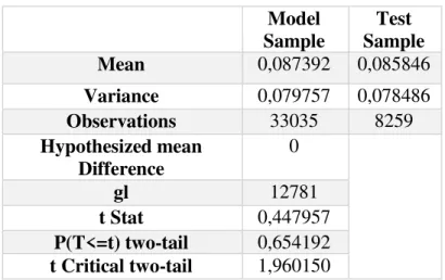
A t-test is required to understand if the difference obtained from the two samples is significant.

(6)

6 Table 2- T Test: two samples with distinguish variances

Model Sample

Test Sample

Mean 0,087392 0,085846

Variance 0,079757 0,078486

Observations 33035 8259

Hypothesized mean Difference

0

gl 12781

t Stat 0,447957

P(T<=t) two-tail 0,654192 t Critical two-tail 1,960150

The T-test analyses the hypothesis that the difference between the mean value of the two samples (model sample and test sample) is zero. The key value on the results table is P two-tail, since the aim is to test the difference between the mean values, which can be negative or positive. The results show clearly that the null hypothesis cannot be rejected, in favor of alternative hypothesis, since the P two-tail value is higher than 5% (P two tails = 65,4%).

The dataset sample is compounded by two files, one with the characteristics of the loan in the original terms, and contains 24 of the variables available (show in secondary appendix Table 1). The second file shows the behaviour of each loan after it is granted on a monthly basis. The last file contains 17 variables and is updated periodically with recent developments on the loan (the variables available can be seen in secondary appendix, Table 2). However, it is important to refer the principal characteristics detected:

Table 3 – Comparison of sample Indicators

Indicators Model

Sample Test Sample

T- test

Difference of Means = 0

Default 8,7392 8,5846 0,6542

LTV 70,2403 70,3735 0,5308

UPB 210 828,5 210 294,5 0,6913

Debt-to-Income 36,3758 36,4013 0,8696

Credit Score 741,4873 741,7707 0,6518

(7)

7

Loan Duration 27,9683 27,9570 0,8543

Original Loan-to Value (LTV) – Is the ratio between the original mortgage loan amount and the minimum value between the mortgaged property’s appraised value and its purchase price. The LTV can be between 6% and 105%. The sample analysis concludes that on average around 70% of the loan is covered by the mortgage value.

Unpaid principal balance (UPB) – Is the amount in debt. At the beginning of the loan this is the amount borrowed. This means that on average the loans from the sample are approximately of 210 500 USD.

Debt-to-Income – Is the sum of the borrower's monthly debt payments, including monthly housing expenses that incorporate the mortgage payment divided by the total monthly income. This is approximately 36%.

Credit Score (FICO) – Freddie Mac use FICO as credit score reference; this value can be between 301 and 850. The average on the sample is approximately 741. This value is high but it is reasonable, since the sample is compounded by the granted loans. This sample already has excluded the “bad clients” (clients that are not given the loan, due to bad FICO score).

Original Interest Rate – Original interest rate is the original interest for the loan. The variable is in percentage. On average the interest rate for the loans in 2008 was 6,05%.

Loan Duration- Loan duration is the time in years that the loan will have until maturity. On average the loans have the duration of approximately 28 years. This make sense because the loans observed are mortgage loans for single families. To be noted that the duration is the time that the agreement establish at beginning of the loan. This duration can be changed.

(8)

8 analysis will be performed to understand the worst FICO score that should be accepted to obtain a 5% Default. After this the test sample will be split by the score obtained on the study, to check if the 5% of Default is accomplished. The same procedure will be used for the alternative model. Once both tests are finalised, it will be possible to compare both results and take conclusions.

CREATION OF THE RULES AND RESULTS ANALYSES

Introduction to FICO Model

FICO score is a credit score model that combines different factors. The secret to this score is the algorithm used, that is based on years of recorded data. The factors used and the approximate weight of each factor are already known:

 Payment History (35%): Payments with small delays have negative impact on the score. Bankruptcies is an example of negative impact on score.

 Outstanding Balances (30%): Having a great deal of money on many accounts or “maxing out” on different credit cards can indicate that person is exceed their limit, and likelihood of making late payments or no payments at all is higher.

 Length of Credit History (15%): The age of a consumer’s oldest and newest credit account. How much time has on average all different credit accounts. Which frequency the accounts are used.

 New Credit (10%): This part of the model looks to the multiple requests for new credit accounts. When someone gets rejected by the lenders, for example, this promotes a negative impact.

 Types of Credit used (10%): The score will consider a credit mix. The score also reflects the impact regarding the number of accounts the person has.

(9)

9 Bank needs to decrease the risk of Default, it will accept the people with higher scores and reject the people with lower scores.

Creation of the rule for FICO Model

The sample has 33.035 Loans, all rated with a FICO score. The minimum score achieved for this sample is 480, which means that people with lower scores were not given credit. The maximum score obtained was 840.

As previously referred, the first objective is to achieve a 5% Default. To obtain this result, the sample was ordered from the highest to lowest score. The next step is to calculate the cumulative default as loans are accepted, until obtaining the 5% default that was set as target. The point where the default passed the 5% threshold was the score 705. Thus, since the FICO score is an integer number and the objective is not cross the 5% threshold, the break point of 706 was established (previous score before 705).

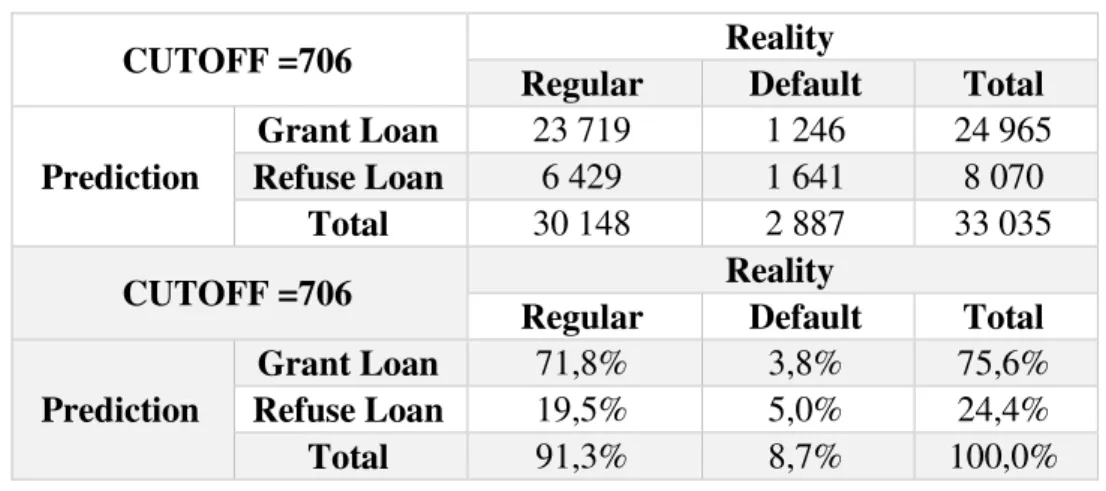
To sum up, loans with scores higher or equal than 706 are accepted and the loans with scores lower than 706 are reject. Based on this rule the sample was distributed as follows:

Table 4 –FICO Model’s Results on Model Sample

CUTOFF =706 Reality

Regular Default Total

Prediction

Grant Loan 23 719 1 246 24 965

Refuse Loan 6 429 1 641 8 070

Total 30 148 2 887 33 035

Prediction

Grant Loan 71,8% 3,8% 75,6%

Refuse Loan 19,5% 5,0% 24,4%

Total 91,3% 8,7% 100,0%

Based on these results some preliminary conclusions can be taken:

(10)

10

 23.719 Loans were accepted and are regular and 1.641 are rejected and should be rejected (loans enter in default).

 The alfa – Type I error (accept a loan that goes into default) is compounded by 1.246 loans.

 The beta - Type II error (reject a loan that would not default) is compounded by 6.429 loans. Thus, the default on rejected population is 18%.

The results obtained are based on the rule created for this dataset. The efficiency of the rule created can only be tested if an independent sample from the same population verifies identical results.

Results of the test sample for FICO Model

The sample has 8.259 Loans that were scored with the FICO score. The minimum score achieved for this sample is 537, higher than that obtained for the model sample.

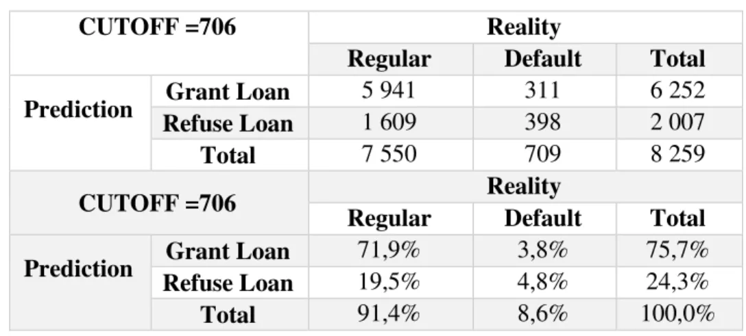
In order of evaluate if the rule previously created is accurate, a test is performed. Applying the cut-off at the score of 706, the results obtained on the sample test are as follows:

Table 5–FICO Model’s Results on Test Sample

Prediction Grant Loan 5 941 311 6 252

Refuse Loan 1 609 398 2 007

Total 7 550 709 8 259

Prediction Grant Loan 71,9% 3,8% 75,7%

Refuse Loan 19,5% 4,8% 24,3%

Total 91,4% 8,6% 100,0%

The conclusions from these results obtained are:

(11)

11

 5.941 Loans were accepted and are regular and 398 are rejected and should be rejected.

 The alfa – Type I error is compounded by 311 loans and represents 4,97% of the total loans accepted.

 The beta - Type II error is compounded by 1.609 loans. Consequentially the default on rejected population is 19,8%.

With the results obtained on the sample test, it will be possible to compare the efficiency of the FICO model with the alternative model, as build in next chapter. This efficiency will be measured by the estimation of the cost of mistakes resulting from the model decision.

Building a New Alternative Model

FICO Model is an existing model. The results obtained by the use of it this model is already on the dataset. Testing the efficiency of the model requires the creation of an alternative model, to compete with FICO.

(12)

12 mean value of different parameters for each of the two populations it is possible to define the line/plan that performs the best split of populations.

In order of choose the best parameters for the model it is required to study the correlation between them. The table showing the correlation between the principal variables (used on the model) is included in appendix A, Table 1.

Based on the correlation table some variables are excluded:

 Original UPB, since it fails the significant test with the delinquency status variable.

 Original Combined LTV, since it is highly correlated to the original LTV; the Original LTV explains the delinquency status variable better than the Original Combined LTV.

The remaining variables were tested for the basis of the model.

After various changes were made to the model, the most appropriate equation to split the two clusters is:

(1) 𝑦 = 𝛽₀+ 0,143 × 𝐿𝑇𝑉 + 0,725 × 𝑂𝑟𝑖𝑔𝑖𝑛𝑎𝑙 𝐼𝑛𝑡𝑒𝑟𝑒𝑠𝑡 𝑅𝑎𝑡𝑒2 + 2,755 ×

𝐶ℎ𝑎𝑛𝑛𝑒𝑙 + 0,118 × Original Debt Income + 0,008 × 𝐿𝑜𝑎𝑛 𝑑𝑢𝑟𝑎𝑛𝑡𝑖𝑜𝑛2

This equation offers the best line to split the two loan populations (regular and delinquency loans). Observations of this equation show that all variables have positive Betas. This happens because all variables contribute to increase y reducing credit quality. Between two loans where a less negative y is observed on the first, the default probability is higher on former. Analyzing the behavior of the equation in further depth, it is observed that the Original Interest Rate and the Loan duration are up to square. This is used in order to worsen the classification obtained on loans with high interest rate and loan duration. Basically the penalty of an additional year, in a loan with 30 years duration has more weight than an additional year on a 10 year loan.

(13)

13 intervenient of the process. The variable varying between no intervenient, a Broker, Correspondent or Third Party Origination involved on the process. For the analysis performed it was noticed that the variable as a graduate impact, noticing that the loans that has a Third Party Origination as more % of default than the ones with correspondent and so on. This way, it was given a punctuations to each different outcome.

Creation of the rule for Alternative Model

Defining 𝛽₀, will cause a variation on the amount of loans with delinquency status that are accepted.

Since the target is to obtain a sample with 5% of delinquency, the corresponding 𝛽₀ =

− 58,63. With this line defined, the rule for acceptance is:

 If 𝑦 < 0 , accept the Loan

 If 𝑦 ≥ 0 , reject the Loan

The maximum value that is obtained for the sample was 28,96 and the minimum obtained was -31,05.

The average result is -3,619 which makes sense, since negative values signify acceptance of the loan and the majority of loans should be accepted.

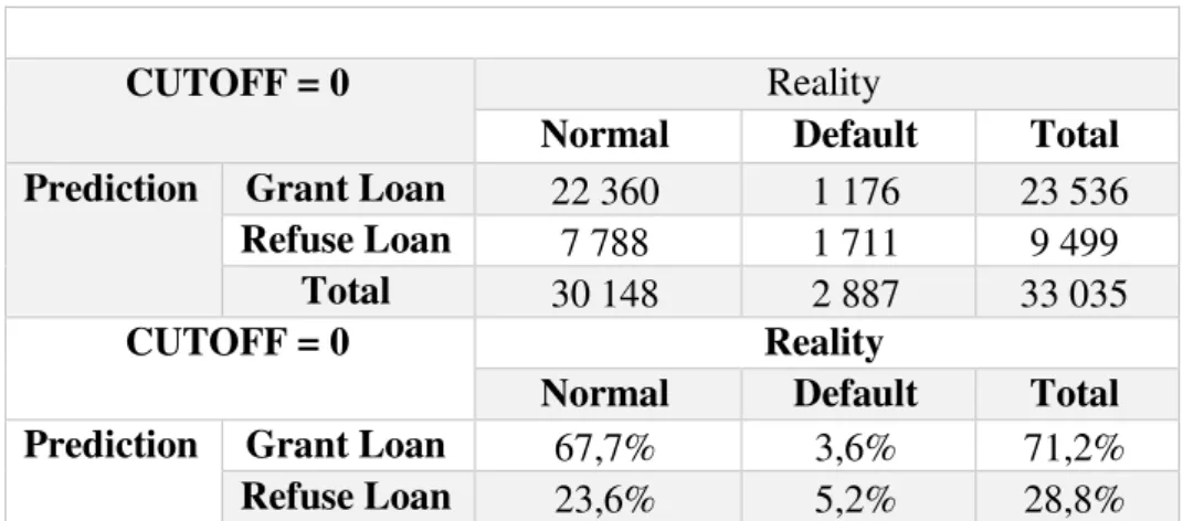
Based on this rule the results for the Model sample are the following: Table 6 –Alternative Model’s Results on Model Sample

CUTOFF = 0 Reality

Normal Default Total

Prediction Grant Loan 22 360 1 176 23 536

Refuse Loan 7 788 1 711 9 499

Total 30 148 2 887 33 035

CUTOFF = 0 Reality

Prediction Grant Loan 67,7% 3,6% 71,2%

(14)

14

Total 91,3% 8,7% 100,0%

Based on the results some preliminary conclusions can be drawn:

 9.499 out of a total of 33.035 Loans were rejected. (28,8% of the sample)

 23.536 Loans were accepted and are regular and 1.711 were rejected and should be rejected.

 The alfa – Type I error is compounded by 1.176 loans.

 The beta - Type II error is compounded by 7.788 loans. With a total rejection of 9.499 loans, the conclusion is that the rejection group has 18% default.

 This model has a lower alfa error than FICO score. However, it has more beta type errors.

Results of the teste sample for Alternative Model

Since the model build is based on a sample, a test is performed to verify if the same results are obtained when the loans are from another sample of the same population. This way it is possible to guarantee that the model results match the behaviour of the population.

Using the equation of the model with the same 𝛽₀, the results obtained from the sample test were as follows:

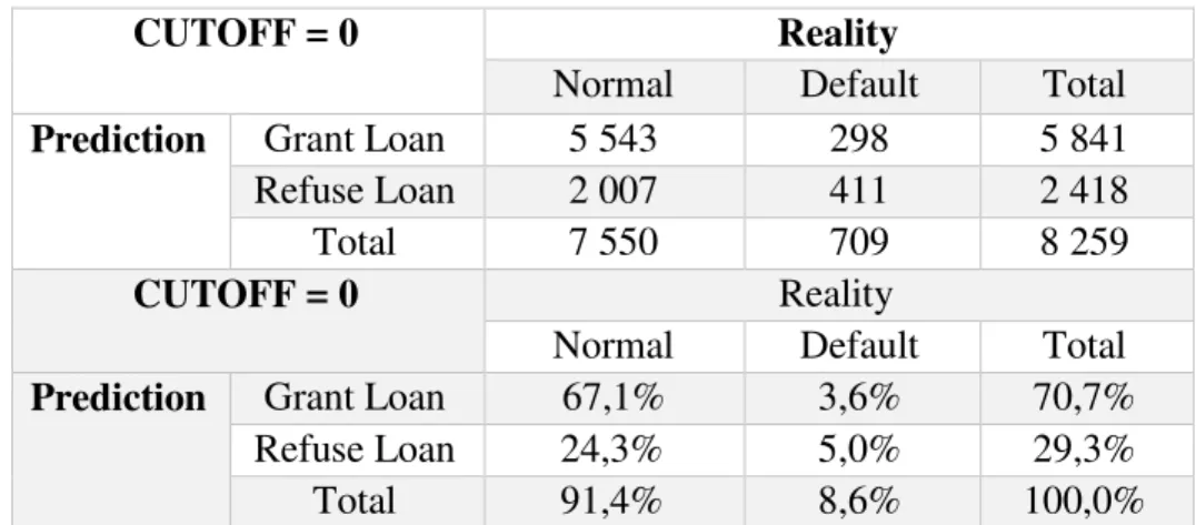
Table 7 - Alternative Model’s Results on Test Sample

CUTOFF = 0 Reality

Normal Default Total

Prediction Grant Loan 5 543 298 5 841

Refuse Loan 2 007 411 2 418

Total 7 550 709 8 259

CUTOFF = 0 Reality

Normal Default Total

Prediction Grant Loan 67,1% 3,6% 70,7%

Refuse Loan 24,3% 5,0% 29,3%

Total 91,4% 8,6% 100,0%

(15)

15 Comparing both Models

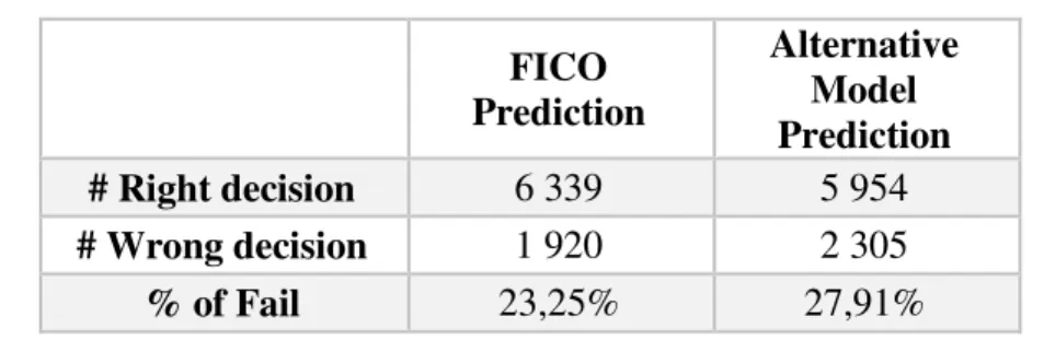
The models analysed have different performances. The performance of these two models, in terms of the number of mistakes occurring, is shown below:

Table 8- Performances Resume

FICO

Prediction

Alternative Model Prediction

# Right decision 6 339 5 954

# Wrong decision 1 920 2 305

% of Fail 23,25% 27,91%

Results shown in the table above conclude that the Alternative Model is worse than the FICO model, although as mention before the models have two types of errors and the different types of mistakes represent different costs to the bank.

If the bank grants a loan and the client doesn’t pay back (alfa error) the bank loses the total amount that the client doesn’t pay. However, if the bank doesn’t grant the loan and the client is a regular client (beta error) the bank is losing the opportunity of earning revenue from the loan margin. The conclusion is that the loss on alfa error is higher than the loss on beta error.

As noted in the previous section, the alfa error is higher if the FICO model is used rather than the alternative model. Thus, to compare both models it is required to calculate the different losses from each model.

(16)

16 During this analysis, it was noticed that some loans had no data regarding the debt variation with time (variable not informed). Thus, an estimate of this was carried out, based on the available information regarding the average percentage of the loan payed before default.

The percentage of loan payed was estimated as follows:

(2) ∑

𝑂𝑟𝑖𝑔𝑖𝑛𝑎𝑙 𝑈𝑃𝐵−𝐶𝑢𝑟𝑟𝑒𝑛𝑡 𝑎𝑐𝑡𝑢𝑎𝑙 𝑈𝑃𝐵𝑑 𝑂𝑟𝑖𝑔𝑖𝑛𝑎𝑙 𝑈𝑃𝐵

𝑁 𝑖=1

𝑁 = 3,75%

Where d is the point in time where default occurs. N the number of loans that enter into default and have this information available.

Based on this, the loan value at the time of default is estimated by the formula: Original UPB* (1-3,75%). Since the data available doesn’t have information on the Loss Given Default (LGD), a value must be assumed. Based on the Portuguese Regulator1 and Basel II2when the LGD is not estimated, an LGD of 45% should be assumed. Having these in mind, the alfa error is estimated as follows:

(3) 𝐿𝑜𝑠𝑠 = 𝑂𝑟𝑖𝑔𝑖𝑛𝑎𝑙 𝑈𝑃𝐵 ∗ (1 − 3,75%) ∗ 45%

To calculate the cost associated to the beta error, the gains associated to each loan granted must be estimated. This value is not included in the information made available. Thus, the banco popular estimates were used.

On average, the bank estimates a gain based on the difference between the interest rate requested and the cost of the money, of each loan per year. To estimate bank gains during the loan:

(4) 𝐺𝑎𝑖𝑛 = (𝑟−𝑐)∗𝑂𝑟𝑖𝑔𝑖𝑛𝑎𝑙 𝑈𝑃𝐵

𝑐−𝑔 ∗ (1 − (

1+𝑔 1+𝑐)

𝑡

)

(17)

17 This formula is a simplification of the method used and (r-c) is the amount that the bank expects to receive from the loan (r represents interest rate practiced by the financial institution). Original UPB is the value of the loan at the start. The g value represents the amortization, since each year the loan is being payed and the amount of gain is thus decreasing, g is consequentially negative (-2%). The t in the formula above represents the time that the loan stays “live”; usually the loan is payed before the maturity date. Since the sample is from 2008, it is not possible to estimate the time that the loan takes. In order to simulate this, 75% of the total time of the loan is assumed. The c the cost of the money. The cost of money is calculated based on the following formula:

(5) 𝐶𝑜𝑠𝑡 𝑜𝑓 𝑚𝑜𝑛𝑒𝑦 = 𝐴𝑑. 𝐶𝑜𝑠𝑡 + (𝐸𝑅𝑂𝐸 ∗ 𝐸𝑞𝑢𝑖𝑡𝑦 ∗ 𝑅𝑊𝐴) +

+𝐹𝑢𝑛𝑑𝑖𝑛𝑔 𝐶𝑜𝑠𝑡 ∗ (1 − 𝑒𝑞𝑢𝑖𝑡𝑦 ∗ 𝑅𝑊𝐴) + 𝐿𝐺𝐷 ∗ 𝑃𝐷

Additional Cost is all administrative cost excluding the funding divided by Total assets of the group. This cost, using estimates from Banco Popular, is approximately 0,7%. The equity considered is 8%, based on Common Equity, from TIER I3. RWA assumed as the standardized approach from Basel II of 35%4. EROE (Expected Return on Equity) is, approximately, 9,5%. This value is estimated based on the equation:

(6) EROE = 𝑟_𝑓+𝛽_𝑖(𝑀𝑎𝑟𝑘𝑒𝑡 𝑅𝑖𝑠𝑘 𝑃𝑟𝑒𝑚𝑖𝑢𝑚 = 9,5%

The risk free was estimated by the average of Treasury Bond 10 Year5 maturity during 2008 and is 3,7%. 𝛽_𝑖 (Beta of the Industry) is 0,896. The Market Risk Premium is 6,5%7. The

3_{Recomencação do Banco de Portugal, Carta-Circular n.º 83/2008/DSB}

4Bank for International Settlements. 2015. “Revisions to the Standardised Approach for credit risk”. http://www.bis.org/bcbs/publ/d347.pdf (accessed April 10, 2016)

5U.S. Department of the Tresaury.2008. “Daily Treasury Yield Curve Rates”.

https://www.treasury.gov/resource-center/data-chart-center/interest-rates/Pages/TextView.aspx?data=yieldYear (accessd May 10, 2016) 6Damodaran Online. 2016. “_{Total Beta By Industry Sector}”.

(18)

18 funding cost, in USA in 2008, was around of 2%8. LGD is 45%, defined previously on error alfa calculations. PD is the probability of default. Since these loans do not enter into Default, a PD of 5%is established as the probability of Default for this sample.

Based on the above information the c applied is:

(7) 𝑐 = 0,7% + 8% ∗ 35% ∗ 9,5% + 2% ∗ (100% − 7,5% ∗ 35%) + 5% ∗

45% ≈ 5,16%

Using the formulas created for the two types of errors, it is possible to compare both models in terms of costs:

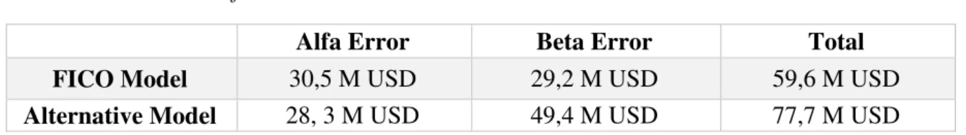
Table 9- Cost of the Models

Alfa Error Beta Error Total

FICO Model 30,5 M USD 29,2 M USD 59,6 M USD

Alternative Model 28, 3 M USD 49,4 M USD 77,7 M USD

Comparing both models, it is observed that FICO is more costly in terms of alfa error, although in terms of Beta error the loss is lower than through the alternative model. With this scenario is clear that the FICO model is preferable to the Alternative model.

Creation of the rule - Models working together

Since both models have distinct behaviours, another alternative is suggested. FICO is the best model, but the alternative is the most appropriate to identify Alfa Errors. It is possible that if both models work together the results can be improved. Based on previous models, the hypothesis of using both models together can be analysed, thus verifying if the performance of default prediction can be improved. Two simple analyses can be carried out:

 If both models agree to accept the loan, the loan is accepted. Otherwise the loan is rejected.

(19)

19

 If both models agree on rejecting the loan, the loan is rejected. Otherwise the loan is accepted.

The 5% default is maintained as a target. In order to achieve 5% default the FICO score and the Alternative model should be adjusted. This one, will decrease the score one point on the former model and will increase one to the latter model. The alternative model will adapt in order to get the 5% of default. This way is analysed if the performance of FICO can be improved or not.

The results of the two analyses are as follows:

Table 10 - Model sample: Both models agree to accept the loan, the loan is accepted

CUTOFF FICO=705; 𝜷0

=-71,9

Reality

Prediction Normal 23 761 1 233 24 994

Default 6 387 1 654 8 041

Total 30 148 2 887 33 035

=-71,9

Reality

Prediction Normal 71,9% 3,7% 75,7%

Default 19,3% 5,0% 24,3%

Total 91,3% 8,7% 100,0%

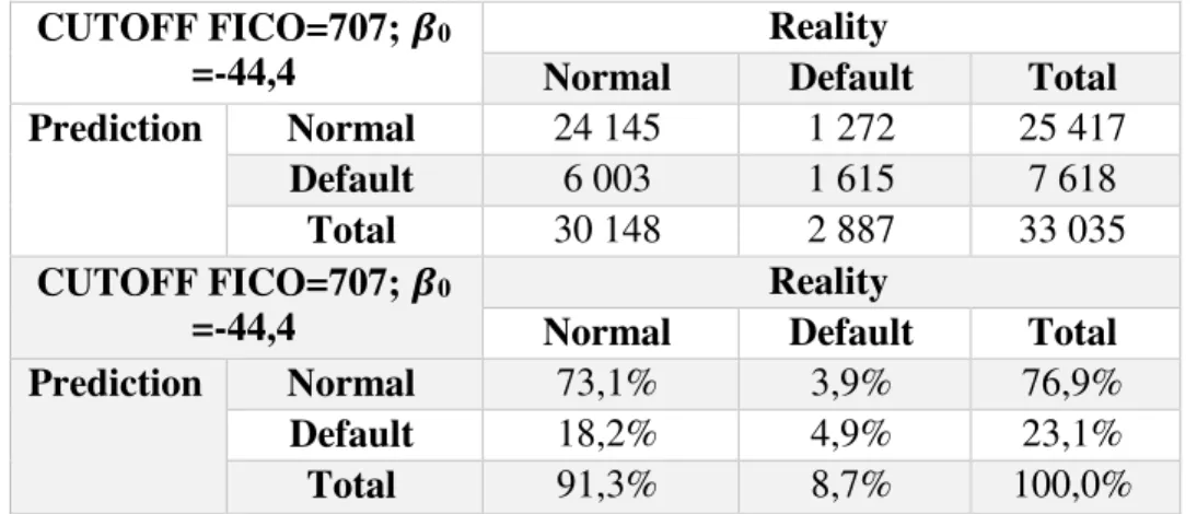
Table 11 – Model sample: Both models agree on rejecting the loan, the loan is rejected

=-44,4

Reality

Prediction Normal 24 145 1 272 25 417

Default 6 003 1 615 7 618

Total 30 148 2 887 33 035

=-44,4

Reality

Default 18,2% 4,9% 23,1%

(20)

20 Comparing the performance of both new models it seems that the latter is the more suitable. However, the former model has a less number of Alfa errors than the latter and the Alfa error is more costly for the bank than the Beta error. To do a suitable comparison should be estimated the cost of each model.

Interpreting the results obtained on the former analyses, the decrease of the FICO score CUTOFF (FICO score alone has the CUTOFF of 706) and the decrease of 𝜷0 of the alternative

model (Alternative model alone has 𝜷0= -58,63) are apparent. Lowering the CUTOFF of FICO

score, the more loans are accepted. The behaviour of 𝜷0 is similar to the FICO, the more negative

is 𝜷0, the more loans are accepted. Thus, both models match regarding acceptance and the target

of 5% default on the sample can be accomplished. If the CUTOFF of FICO and 𝜷0 do not differ

from the individual model performances, the results would show default values below 5% but higher percentage of rejection of loans.

For the latter model, the opposite behaviour is observed. The CUTOFF of FICO increases and the 𝜷0 is less negative. If the CUTOFF on the FICO score increases, rejection is higher. The

same happens if 𝜷0 is less negative. It is thus possible to match more rejected loans. If the

CUTOFF of FICO and 𝜷0 not differ from the individual model performances, the results would

show defaults above 5% but a lower percentage of loan rejection.

Testing the models working together

Since the models built are based on a sample, tests are performed to verify if the same results are obtained when the loans originate from another sample of the same population.

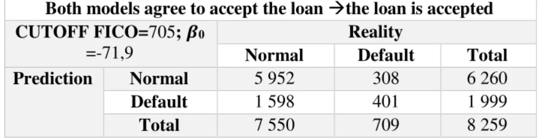
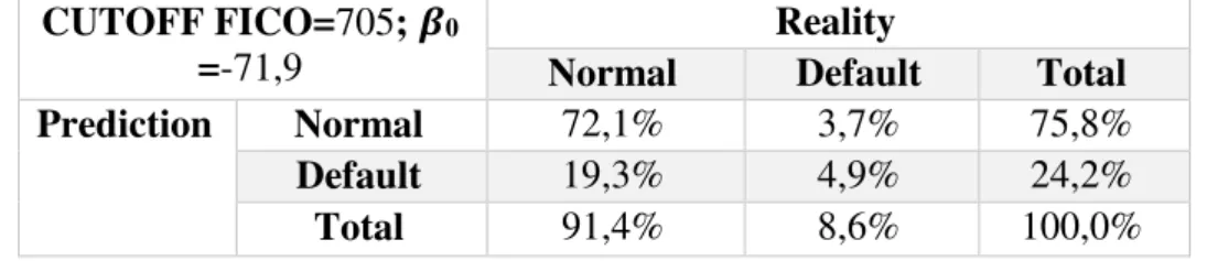
Table 12 - Test sample: Both models agree to accept the loan, the loan is accepted

Both models agree to accept the loan the loan is accepted CUTOFF FICO=705; 𝜷0

=-71,9

Reality

Prediction Normal 5 952 308 6 260

Default 1 598 401 1 999

(21)

21 CUTOFF FICO=705; 𝜷0

=-71,9

Reality

Default 19,3% 4,9% 24,2%

Total 91,4% 8,6% 100,0%

Table 13 - Test sample: Both models agree on reject the loan, the loan is rejected

Both models agree on reject the loan the loan is rejected CUTOFF FICO=707; 𝜷0

=-44,4

Reality

Prediction Normal 6 023 316 6 339

Default 1 527 393 1 920

Total 7 550 709 8 259

=-44,4

Reality

Default 18,5% 4,8% 23,2%

Total 91,4% 8,6% 100,0%

Comparing both performances with FICO score working alone, it is noticeable that both new models have a lower rejection than the FICO score working on its own. However, both models have a higher number of loans contributing to the alfa error. The Alfa error is more costly than the Beta Error.

Based on the previous formulas the cost for these two new performances are estimated and compared with the models working alone:

Table 14 -Cost of the Models

Alfa Error Beta Error Total

FICO Model 30,5 M USD 29,2 M USD 59,6 M USD

Alternative Model 28, 3 M USD 49,4 M USD 77,7 M USD

FICO Model + Alternative Model

Accept

30,3 M USD 29,3 M USD 59,6 M USD

FICO Model + Alternative Model

Reject

(22)

22 From this last table it is observed that the difference between performances is not significant. Only the alternative model showed to be more costly.

LIMITATIONS AND IMPROVEMENTS

Limitations

The Sample for the analysis was extracted from Freddie Mac website. The dataset is compounded by active data. This means that the information suffers updates throughout time. The study should take this matter into account, as this influences the accuracy of conclusions and can lead to errors. Another important fragility of the study is that it is only possible to analyse the loans that were accepted by Freddie Mac at the time and no information is available on the rejected loan requests. This means that the sample has already been treated. The study assumes that the samples available represent the behaviour of all the population.

The sample used is based on a USA dataset. The behaviour of Loans in Portugal is different to the behaviour in the USA. For Banco Popular, the use of the FICO model will require tests from performance in Portugal.

Legislation in Portugal has restrictions on the use of defaults non banking (such as default on payment of electricity). These limitations on available information can affect the performance of FICO.

The following types of mortgages were excluded by Freddie Mac, from the Dataset:

 Adjustable Rate Mortgages;

 Refinance Mortgages;

 Government-insured mortgages, comprising Federal Housing Administration, Guaranteed Rural Housing;

 Mortgages carried by Freddie Mac as a consequence of alternate agreements;

(23)

23

 Mortgages associated to Mortgage Revenue Bonds;

 Mortgages carried by Freddie Mac that has credit enhancements despide primary mortgage insurance.

Improvements

The FICO score proves to be efficient. However, it shows that a small variance on the score can make a big difference on the percentage of default. On a next phase of the study it is recommend develop a model where the decision can be rejected, accepted or further analysed. This third option arises when the scores are at limit situations, such as between the score of 704 and 708. When the score is within this gap, the analyst should take the decision based on parameters that are not FICO score (alternative model for instance).

RECOMMENDATIONS

This study explores how the default prediction Model FICO, for a Single Family Loans, behaves when compared to alternative models. We believe that this study has a high practical value, given that it explores the possibility of prediction models working together and gives a perspective on how this can be achieved. Thus, this study expects to create awareness on how different models can affect the performance of the financial entities.

Considering the results obtained during this study, it is proved that the FICO score is a good prediction model and that the performance of financial entities can be easily improved by defining a limit score which is more or less restrictive. It is important to note that the FICO performance test is limited to the information available and that application of this performance test in Portugal can have some discrepancies.

(24)

24

APPENDIX A

Table 15 - Variables Correlation

ORIGINA

L_DEBT- TO-INCOME

ORIGINAL_

LOAN-TO-VALUE

ORIGINA L_INTERE

ST_RATE

CHANNE L

LOAN _DUR ATIO

N

DELIQUENCY _STATUS ORIGINAL_

DEBT-TO-INCOME

1,000 0,165 0,149 0,058 0,143 0,137

ORIGINAL_

LOAN-TO-VALUE

0,165 1,000 0,208 0,022 0,233 0,133

ORIGINAL_ INTEREST_R

ATE

0,149 0,208 1,000 -0,060 0,284 0,171

CHANNEL 0,058 0,022 -0,060 1,000 0,008 0,080

LOAN_

DURATION 0,143 0,233 0,284 0,008 1,000 0,076

DELIQUENC

(25)

25 REFERENCES

Allen N. Berger, Christa H.S. Bouwman. 2013. “How does capital affect bank performance during financial crises?” Paper presented at the Journal of Financial Economics. Volume 109

Banco de Portugal. 2008. “Carta-Circular n.º 83/2008/DSB”. http://www.bportugal.pt/sibap/application/app1/docs1/circulares/textos/83-2 (accessed May 6, 2016)

Bank for International Settlements. 2015. “Revisions to the Standardised Approach for credit risk”. http://www.bis.org/bcbs/publ/d347.pdf (accessed April 10, 2016)

Brealey, R. A., S. C. Myers, and F. Allen. 2005. “Principles of Corporate Finance” 8th edition, McGraw-Hill/Irwin.

Damodaran Online. 2016. “Total Beta By Industry Sector”. http://people.stern.nyu.edu/adamodar/New_Home_Page/datacurrent.html (accessed May 6, 2016)

Federal Reserve Bank of New York .2008. “Federal Funds Data”. https://apps.newyorkfed.org/markets/autorates/fed%20funds (accessed May 6, 2016)

Fernández, P. 2009. “Market Risk Premium Used in 2008: A survey of more than a 1000 professors”. Master Dissertation. IESE Business School – University of Navarra.

Freddie Mac. 2008. “Loan-Level Dataset”.

Sample_orig_2008.http://www.freddiemac.com/news/finance/sf_loanlevel_dataset.html (accessed February 21, 2016)

Freddie Mac. 2008. “Loan-Level Dataset”. Sample_svcg_2008. http://www.freddiemac.com/news/finance/sf_loanlevel_dataset.html (accessed February 21, 2016)

U.S. Department of the Tresaury.2008. “Daily Treasury Yield Curve Rates”.