www.biogeosciences.net/6/2847/2009/
© Author(s) 2009. This work is distributed under the Creative Commons Attribution 3.0 License.
Biogeosciences
Estimation of NH
3
emissions from a naturally ventilated livestock
farm using local-scale atmospheric dispersion modelling
A. Hensen1, B. Loubet2, J. Mosquera1,*, W. C. M. van den Bulk1, J. W. Erisman1, U. D¨ammgen3, C. Milford4, F. J. L¨opmeier3, P. Cellier2, P. Mikuˇska5, and M. A. Sutton4
1Energy research Centre of the Netherlands (ECN), Petten, The Netherlands
2Institut National de la Recherche Agronomique (INRA), Thiverval-Grignon, France 3Federal Agricultural Research Centre, Braunschweig (FAL), Germany
4Centre for Ecology and Hydrology (CEH), Edinburgh, UK
5Institute of Analytical Chemistry, ASCR, v.v.i., Brno, Czech Republic *now at: Animal Sciences Group (ASG), Wageningen, Germany
Received: 11 September 2008 – Published in Biogeosciences Discuss.: 14 January 2009 Revised: 14 September 2009 – Accepted: 16 September 2009 – Published: 4 December 2009
Abstract. Agricultural livestock represents the main source of ammonia (NH3) in Europe. In recent years, reduction
poli-cies have been applied to reduce NH3emissions. In order to
estimate the impacts of these policies, robust estimates of the emissions from the main sources, i.e. livestock farms are needed. In this paper, the NH3 emissions were estimated
from a naturally ventilated livestock farm in Braunschweig, Germany during a joint field experiment of the GRAMINAE European project. An inference method was used with a Gaussian-3D plume model and with the Huang 3-D model. NH3 concentrations downwind of the source were used
to-gether with micrometeorological data to estimate the source strength over time. Mobile NH3concentration measurements
provided information on the spatial distribution of source strength. The estimated emission strength ranged between 6.4±0.18 kg NH3d−1 (Huang 3-D model) and 9.2±0.7 kg
NH3d−1(Gaussian-3D model). These estimates were 94%
and 63% of what was obtained using emission factors from the German national inventory (9.6 kg d−1NH
3). The effect
of deposition was evaluated with the FIDES-2D model. This increased the emission estimate to 11.7 kg NH3d−1,
show-ing that deposition can explain the observed difference. The daily pattern of the source was correlated with net radiation and with the temperature inside the animal houses. The daily pattern resulted from a combination of a temperature effect on the source concentration together with an effect of vari-ations in free and forced convection of the building
venti-Correspondence to:A. Hensen ([email protected])
lation rate. Further development of the plume technique is especially relevant for naturally ventilated farms, since the variable ventilation rate makes other emission measurements difficult.
1 Introduction
Atmospheric ammonia (NH3)is recognized as a major
pol-lutant impacting on sensitive ecosystems (Bobbink et al., 1992). NH3 deposition may indeed cause soil acidification
through nitrification processes (van Breemen et al., 1982), although this depends upon the biological and chemical sta-tus of the soil on which it is deposited, and upon the form of NHxdeposited (NH3or NH+4)(Galloway, 1995).
Further-more, atmospheric inputs of NHxmay induce eutrophication
of sensitive ecosystems, as well as decrease their biodiversity (Heij and Schneider, 1991; Bobbink et al., 1992). Agricul-ture is the main source of NH3in Europe (Asman, 1992; Heij
and Schneider, 1995), and represents more than 80% of the total anthropogenic input at the global scale (Bouwman et al., 1997). The inventory studies of Pain (1990), of Pain et al. (1998) and D¨ohler et al. (2002) show that cattle represents the largest source of agricultural NH3emissions in Europe.
100 300 500 700 900 1100
Site 1
Site 2
Buildings Sources
Other Grassland Measurement locations
Arable land Main sampling site
Wood & Sub-urban Main Field (grass)
Roads DWD meteo field
Transect measurement
Main Field
“Kleinkamp”
Site 3
Grass field II
Farm area
Site 5
N
1300 1500
Site 6
BackgroundTower
-300 -100 100 300 500 700 900 1100 1300 1500 1700 1900
Distance (m)
Site 7
Meteo data Testcrop
Site 4
sub-urban housing
PTB
K
J
I
E
C
A
B
H FG
Grass field III
Grass field IV
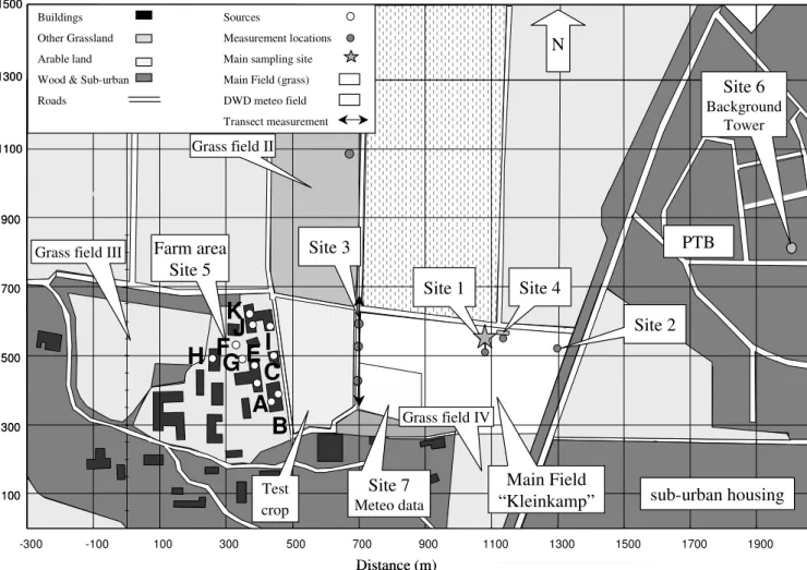
Fig. 1. Overview of the measurement site. The three locations of NH3air concentration measurement (grey circles) used in this analysis are indicated as Site 1, Site 2 and Site 3. The plume transect measurements were made along the track at Site 3. The sources buildings are labelled from A to K (see Table 1). Distances are shown on the axes of the map in meters (For further description of the site, see Sutton, 2009a).
Measurement of NH3emissions from naturally ventilated
animal houses is technically complex, expensive, and labour intensive (Phillips et al., 2001; Scholtens et al., 2004; Welch et al., 2005a, b). This is primarily due to difficulties in determining the ventilation rate, which varies according to temperature, wind speed, building design, orientation to the wind and animal occupancy (Zhang et al., 2005; Welch et al., 2005b), but also to difficulties inherent in accurately measur-ing the ammonia concentration on short-time basis (Phillips et al., 2005). However, methods such as the internal or ex-ternal tracer-ratio techniques or the flux-sampling technique have been successfully tested under real conditions (Dem-mers et al., 2001; Dore et al., 2004).
Dispersion models can be used as tools to estimate am-monia emissions from animal houses. Among them, the Gaussian-3D model, assuming constant wind-speed (U )and diffusivity (Kz) withzis widely used because of its simplic-ity (Gash, 1985). Analytical models that include variation of
U andKzwith height also exist (e.g., Smith, 1957; Philip, 1959; Yeh and Huang, 1975; Huang, 1979; Wilson et al., 1982). The technique using Gaussian models to infer NH3
source from a farm building has been reported in Mosquera et al. (2004). Lagrangian stochastic models have also been tested to infer sources of tracers from concentration measure-ments downwind of sources such as animal houses (Flesch et al., 2005) cattle feedlots (Flesch et al., 2007) and fields (Lou-bet et al., 2006; Sommer et al., 2005). More complex Eule-rian models have also been used and validated against ex-tensive measurements for estimating emissions of NH3from
buildings (Welch et al., 2005b).
with inventory emission factors. The daily variability of the emissions is analyzed in comparison with environmental fac-tors such as indoor temperature, external radiation and wind speed. The inferred emission strengths are used in a compan-ion paper (Loubet et al., 2006) as inputs for quantifying the local advection errors induced by the plume coming from the farm on NH3 fluxes measured over a grassland site nearby.
This study was performed within the framework of the Euro-pean project GRAMINAE.
2 Materials and methods
2.1 Measurement site
The field site is a 12 ha experimental grassland situated in the grounds of the Federal Agricultural Research Centre (FAL), Braunschweig, Germany. Directly adjacent to the field are an experimental farm of the FAL and a station of the German Weather Service (Deutscher Wetterdienst). A more detailed description of the site can be found in Sutton et al. (2009a)
The main source of ammonia in the area is the set of farm buildings A–K (Fig. 1). The distance from west to east is namedx, whereas the distance from south to north is called
y, and height above ground isz. The distance between the downwind edge of the farm building area and the different sites are: 230 m for Site 3 where plume measurements were done, and 610 m for Site 1, were micrometeorological mea-surements were done. The farm buildings themselves oc-cupy an area of approximately 180 m (E-W)×300 m (S-N). Table 1 gives an estimate of the yearly NH3 emission for
each building identified in Fig. 1, based on the emission factors of D¨ohler et al. (2002) which can be compared to measurement-based estimates emissions factors from Dem-mers et al. (2001) in Great-Britain, which are 3.5 and 8.9 kg NH3animal−1year−1, for beef and dairy cattle, respectively.
2.2 Concentration measurements
The locations of ammonia concentration measurements are shown as grey dots in Fig. 1. Three AMANDA rotating wet denuders (Wyers et al., 1993) were placed along the N-S tran-sect at Site 3, which gave NH3concentrations on a 15 min
averaging period at 1 m height. These instruments were also used to calibrate a fast-response mobile NH3analyser, itself
being moved along the North-West line on the adjacent track (marked as Site 3 in Fig. 1), to measure the plume cross-section at 1.5 m height. The background NH3concentrations
were measured with a batch denuder system, located at 42 m height on the top of a tower (Site 6 in Fig. 1), which was lo-cated at approximately 1600 m East-North-East of the farm and 800 North-East of the grassland. Mean and standard de-viation of the concentration were estimated for Site 3 over the three measurement systems.
For the mobile measurements, a fast response AMANDA sensor was used, with a time resolution of 30 s. This
sys-tem, described in Erisman et al. (2001), is essentially similar to an AMANDA, but the liquid flow is higher (10 ml min−1 instead of 1.6 ml min−1). However, it does not give an abso-lute concentration, and therefore requires regular calibrations against a reference. The fast response sensor was placed on a trolley and moved along a track through the plume cross-section, and calibrated against the three AMANDA sensors on the same transect (Fig. 1). Note that the calibration was done on differing integration time, as the AMANDA inte-grates over 15 min. Four subsequent transects were used to evaluate the emission strength with these data.
2.3 Micrometeorological measurements
Micrometeorological measurements were performed at Sites 1 and 2. The consensus micrometeorological database derived from the range of measurements performed and de-tailed in Nemitz et al. (2009) was used in this study. The wind-speed (U ), wind-direction (WD), friction velocity (u∗), Monin-Obukhov length (L), and sensible heat fluxes (H ), were derived from several ultrasonic anemometer measure-ments. The latent heat flux (LE) was derived from eddy co-variance measurements using the ultrasonic anemometers in combination with a close-path H2O analyser (Licor 6262) or
open-path H2O analyser (KH2O). Air temperature (Ta),
rel-ative Humidity (HR) and global (Rg)and net radiation (Rn)
were also used.
3 Inference of the source strength from NH3
concentration
3.1 General approach
In this paper, we compare two models: a 3-D Gaussian plume model that assumes a constant wind speed (U )and diffusivity (Kz)everywhere and the Huang (1979) 3-D model
(Huang-3D) that assumes that bothU andKz are power low
func-tions of height, and a plage source. Moreover, the FIDES-2D model, which is also based on Huang (1979) but assumes cross-wind homogeneity of the source (see Loubet et al., 2001, for details) is also used to estimate the potential er-ror made by neglecting deposition or emission of NH3from
nearby fields.
Three inference methods were used to estimate the source strength variability in space and time:
1. The Gaussian-3D model was used in conjunction with mobile NH3 measurements to estimate the source
strength, based on a source distribution equivalent to the emission inventory.
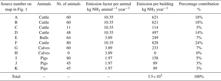
Table 1. Description of the farm animal houses, along with their potential emission estimated using German national emission factors (D¨ohler et al., 2002) and inventoried number of animals. The total yearly emission of the source is 3.5×10³kg year−1NH3and the total
number of animals is 553. The corresponding average daily total emission is 9.6 kg d−1NH3.
Source number on Animals Nr. of animals Emission factor per animal Emission per building Percentage contribution
map in Fig. 1 kg NH3animal−1year−1 kg NH3year−1 %
A Cattle 60 10.35 621 18%
B Cattle 60 10.35 621 18%
C Cattle 11 10.35 114 3%
D Cattle 48 10.35 497 14%
E Bulls 64 3.89 249 7%
F Cattle 80 10.35 828 24%
G Calves 60 3.89 233 7%
H Calves 0 3.89 0 0%
I Pigs 80 1.97 158 5%
J Pigs 45 1.97 89 3%
K Pigs 45 1.97 89 3%
Total – – – 3.5×10³ 100%
3. The Huang-3D and the Gaussian-3D model were used in conjunction with 15 min NH3 concentration
mea-sured at Site 3 to estimate the time course of the emis-sions, knowing its spatial variability.
The basic hypothesis made in these approaches are: (a) un-less specified, no NH3deposition is included, as it is
consid-ered to be of secondary importance compared with the effect of dispersion on the concentration (e.g., Loubet and Cellier, 2002); (b) no chemical reactions are envisaged, as again the effect on the overall NH3 concentration is not expected to
be large on such a small scale (Nemitz et al.; 2009); and (c) the surface characteristics are considered to be homoge-neous (i.e., z0,d), since the models used cannot deal with
varying surface roughness, though this is considered to be of minor importance when compared with the potential pertur-bations induced by the buildings.
With each of the models, the approach is based on the general superposition principle (e.g., Thomson, 1987; Rau-pach, 1989), which relates the concentration at a location (x,y,z),χ (x,y,z), to the source strength at another location (xs, ys, zs),Sfarm(xs, ys, zs), with the use of a dispersion
functionD(x, y, z / xs,ys, zs)(in s m−3): χ (x,y,z)=χbgd+
Z
allxsandys
Sfarm(xs,ys,zs)D(x,y,z|xs,ys,zs)dxs
(1) whereχbgdis the background concentration, assumed to be
constant with height. The three models are different in the way they calculate the dispersion functionD(x,y,z|xs,ys, zs)and the different approaches are detailed in the following.
In the following the dispersion function will be writtenD(x,
y,z)for simplicity.
3.2 The Gaussian-3D model
The Gaussian-3D model is based on the assumptions thatU
andKzare constant in the whole domain, which implies that χ (x, y, z) is a function of two independent Gaussian dis-tributions in the horizontal and the vertical planes (see e.g. Lin and Hildemann, 1997). The contribution from a single source located at (xs,ys, zs)to a point receptor located at (x, y, z)is the dispersion functionD(x, y, z/xs,ys, zs), which
was calculated usingX=x–xsandY=y–ys, as:
D(X,Y,z)= Q
2π·σy·σz· e−Y2
(2·σy)2
·e−(z−zs)2(2·σz)2+e−(z+zs)2(2·σz)2 (2) σy=g·Xh·zo0.2·T0.35
σz=c·Xd·(10·zo)0.53·e e=X−0.22
(3)
whereQis the source strength (in g s−1NH3),zs the height
of the source (animal house) (in m),σy andσzare the
stan-dard deviation of the lateral and vertical concentration dis-tribution respectively (in m),zois the roughness length (in
m),T is the averaging time, and the parametersg,h,candd
are dependent on the stability classes as detailed in Pasquill (1974). The model used is a multiple plume model based on the superposition of several Gaussian plumes each described by Eqs. (2–3). The concentration at each receptor is the sum of the contribution of all the sources according to Eq. (1). The downwind (X)and crosswind (Y )distances are calcu-lated for each source-receptor couple as follows:
X= −(x−xs)·sin(wd)−(y−ys)·cos(wd)
3.3 The Huang-3D plage source model
In this model based on Huang (1979),D(x, z/xs, zs)is
eval-uated from a solution of the advection-diffusion equation ob-tained assuming power law functions forU (z)andKz(z):
U (z)=azp Kz(z)=bzn
D(X,Y,z)= Q
σ y√2πexp
−2(Y )σ y22
×(zhs)bαX(1−n)/2
×exp−a(zα+hsα)
bα2X
×I−υ
2a(zhs)α/2
bα2X
σ y=√1
2Cyx
2−m
2
(5)
Whereα=2+p+n,ν=(1–n)/α, andI−νist the modified Bessel
function of the first kind of order−ν, andCy andmwere
determined from Sutton (1932). The values ofa,b,pandn
were inferred by linear regression between ln(U ), ln(Kz)and
ln(z), over the height 2×z0–20 m, usingU (z)andKz(z)
es-timated from the Monin-Obukhov similarity theory (see e.g. Kaimal and Finnigan, 1994). Since the model uses stability corrections, its use is limited to values of the Monin Obukhov length (L)and the friction velocityu∗such that|L|>5 m and
u∗>0.2 m s−1. In this model, the source is assumed to be a plage source of size 180 m inx and 300 m in y located at 230 m upwind from Site 3 (where concentration is mea-sured).
3.4 The FIDES-2D model
The FIDES-2D model was used to evaluate the influence of deposition and emission of NH3from downwind fields on the
estimation of the source strength. FIDES-2D is based on the two-dimensional dispersion model of Huang (1979), which is hence an integration of Eq. (5) over y. The dispersion model is coupled with a surface resistance model as detailed in Loubet et al. (2001). The equivalent 2-D source was con-sidered 180 m long inxand infinite iny. The source strength per unit area inferred with FIDES-2D has been multiplied by the equivalent surface of the source: 180 m×300 m.
3.5 Spatial distribution of the farm emissions with the Gaussian 3-D model
The Gaussian-3D model was used to infer the source strength of the farm buildings, using the ammonia concentration mea-sured at the three fixed points at Site 3 (AM1..3). The
Gaussian-3D model was run in forward mode to estimate the contribution of the eleven sources in Table 1 to the three receptor concentration levels. The sum of the eleven time series is compared with the measured data. The eleven emission levels were modified using the EXCEL (Microsoft) solver function optimizing the correlation coefficient be-tween the measured and modelled concentration time series. The emission strength of the whole farm areaSfarm was
cal-0.0 1.0 2.0 3.0 4.0 5.0 6.0 7.0 8.0 9.0 10.0
-6
0
-1
0
40
90
14
0
19
0
<--- South Space (m) North ---->
NH
3
co
n
cen
tr
at
io
n
s
(μ
g m
-3)
North to South (12:00) Model 12:00 AM1-3 12:00 North to South (14:00) Model calc 14:00 AM1-3 14:00
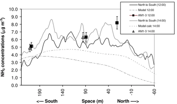
Fig. 2. Two fast-sensor measurements of the NH3plume cross-section at Site 3 the 12 June 2000 at 12:00 and 14:00. The simul-taneous concentrations measurements obtained with the 3 station-ary AMANDA systems (AM1..3)are shown at their
correspond-ing locations in the plume. The figure also shows the plume mod-elled with the Gaussian-3D model using the source distribution and strength as given in Table 1. The difference between the fast sensor and the stationary AMANDA concentrations is mainly due to the time response of the AMANDA being 15 min while the fast sensor has a 30 time response. For the N-S axis, 0 m corresponds to the intersection with the main E-W track N of Kleinkamp (Fig. 1).
culated for each 15 min measurement intervalt at the indi-vidual receptor locations (AM1..3)using:
Sfarm(t,AMi)=Qinput×
χmeasured(AMi)−χbgd
χmodel(AMi)
(6) whereQinput is the initial source strength used to estimate
χmodel, AMi=(AM1, AM2or AM3)are the receptor locations
at Site 3. The time-average and standard deviation ofSfarm
was then estimated at each receptor locations AM1..3. The
emission from the farm site were evaluated using all mea-surements with a wind direction between 200◦and 340◦. 3.6 Time course of the farm emissions
To evaluate the time course of the farm emissions, the av-erage concentration at Site 3 (over the three sensors)χmeas
(Site 3) was used. The Huang-3D, FIDES-2D and the Gaussian-3D model were all used in the same manner to eval-uate the source strengthSfarmsimply as:
Sfarm(t )= (χmeas(Site 3)−χbgd)
D(XSite3,YSite3,z=1m)
(7) WhereXSite3andYSite3are the coordinates of Site 3, andDis
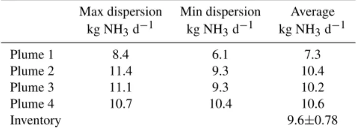
Table 2.Emission estimates using 4 plume transects measured with the fast response sensor (12 June 2000). Uncertainty of the mean is given as standard error.
Max dispersion Min dispersion Average kg NH3d−1 kg NH3d−1 kg NH3d−1
Plume 1 8.4 6.1 7.3
Plume 2 11.4 9.3 10.4
Plume 3 11.1 9.3 10.2
Plume 4 10.7 10.4 10.6
Inventory 9.6±0.78
4 Results
4.1 Spatial variability of the farm emissions inferred with the fast response NH3sensor
Figure 2 shows two NH3 concentration transects across the
plume coming from the farm, obtained with the fast response sensor at Site 3. The transects were obtained at midday from 12:00 to 14:00 on 12 June. The absolute concentration differs slightly between the two periods, which could be explained on the basis of differences in wind-speed.
Four plumes obtained with the mobile measurements sys-tem were used to evaluate the emission of the farm site. A set of two model runs was performed using the source distribu-tion in Table 1. The potential for large and small initial mix-ing close to the farm area was evaluated by settmix-ing an initial horizontal dispersion at the farm source of either 50 or 10 m. Initial dispersion in the vertical direction was set to 5 m. The two model runs provide concentration patterns along the transect that were compared with the measured concentra-tion levels. The source estimates for the four plumes and two model runs are shown in Table 2. The emission needed in the model to make the output fit with the measurements is about 10% higher for the plumes 2–4 compared with the inventory source strength. Including plume 1, the emission estimate equals the inventory estimate at 9.6 kg NH3d−1.
The mobile plume measurements show the shape of the plume providing information on the lateral dispersion. The model runs for these plumes showed that the lateral disper-sion in the model corresponds with the measurement data at a roughness lengthzo=0.2 m. The mobile measurements
only covered a small time-period and were hard to do during the night. Therefore, the spatial distribution of the sources within the farm area was evaluated further using the three AMANDA stations AM1–AM3at Site 3. Using the source
distribution of Table 1 (emission inventory), and tuning the overall source strengthSfam, the modelled and measured
con-centration patterns for the three AMANDA locations showed low correlation coefficients of R=0.36, 0.30 and 0.20, re-spectively (Table 3). The model calculations were used to
obtain insight in the source-receptor relation for each mea-surement location. Sources A, B, D and F give the highest contribution to the modelled signal at the three receptor lo-cations. The time series of the estimatedSfarm (Eq. 5) were
used to estimate the average, standard deviation and median (Table 3). The average emission level obtained in this way was 9.8±0.8 kg NH3d−1, which is close to the expected level
of 9.6 kg NH3d−1. The uncertainty range of 0.8 kg NH3d−1
was obtained from the standard errors in Table 3. The stan-dard deviation of the source estimate is about 100% this is a combination of uncertainty in the method and of the actual temporal variation of the source strength (discussed below).
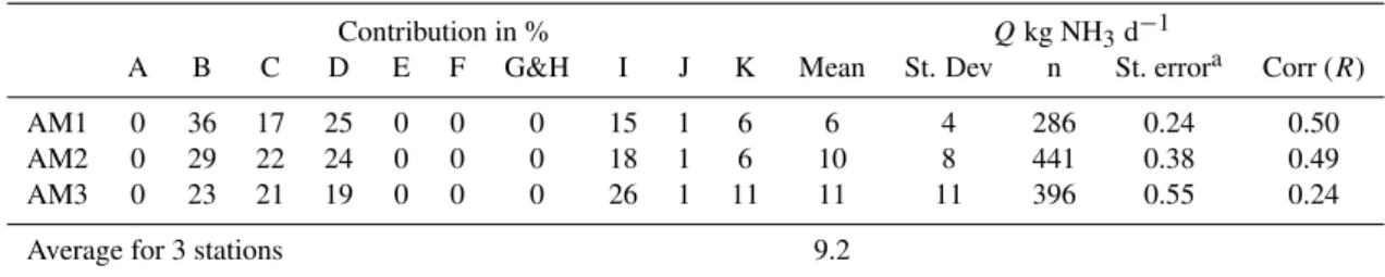
In a second step, the correlation between the measured and modelled concentration pattern at Site 3 was optimised by modifying the source distribution. The results are shown in Table 4. The source distribution estimated by this means shows a decreased contribution from sources A, E and F, and an increase in the emission from B and C. The correlation between measured and modelled concentration patterns in-creased toR=0.5 and 0.49 for stations AM1 and AM2. No significant effect is observed for AM3. The revised total source strength estimate obtained from the time-series at this source distribution is 9.2 kg NH3d−1. Accounting for
sim-ple uncertainty in estimates by system AM1-3 (n=3) gives a standard error of 1.6 kg NH3d−1, which gives a conservative
estimate of the uncertainty. Conversely, given the large sam-ple sizes (n=286 to 441), standard errors for the individual AMANDA systems are in the range 0.2–0.6 kg NH3d−1.
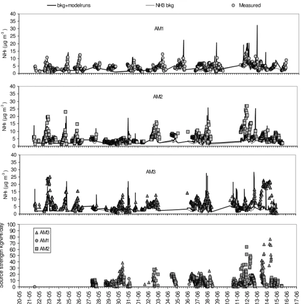
Figure 3 shows an illustration of the measured and mod-elled concentrations using the Gaussian-3D model for AM1-3 at Site AM1-3 over a two-day period using the adjusted source distribution. The correlation coefficient in Table 4 shows that 10–25% of the temporal variation can be explained. The dif-ferences are expected due to the assumption of a constant source-strength with time. This shows that the combination of time variation in meteorological conditions and the spatial variability of the source can explain part of the variability in the concentration, but not all.
Table 5 gives the estimated source strength using the Gaussian-3D model, as well as the source strength estimated using the emission factors of D¨ohler et al. (2002). The modi-fication in the source distribution, which was done in order to increase the correlation between measurements and model, suggests that the sources in the south have a low emission, whereas the sources in the north are a factor 3–5 higher. For building A, E, G the Gaussian-3D model significantly un-derestimates the relative source strength, whereas it overesti-mates for buildings C,D, I, and K.
4.2 Temporal variability of the farm emissions esti-mated with the Huang 3D model
Figure 4 shows an example result of inferred source strength (kg NH3day−1)using the Huang-3D model for the
Table 3.Source-receptor relation and source estimate obtained with the Gaussian-3D model using the spatial source distribution as obtained using the inventory data.
Contribution in % Qkg NH3d−1
A B C D E F G&H I J K Mean St. dev N St. errora Corr (R)
AM1 26 30 3 9 4 13 3 6 2 2 7 4 456 0.19 0.36
AM2 22 26 4 11 6 15 4 7 3 3 10 10 568 0.42 0.30
AM3 18 23 4 10 6 19 5 8 3 4 12 14 459 0.65 0.20
Mean for 3 stations 9.8
astandard error =st. deviation/sqrt(n)
Table 4.Source-receptor relation and source estimate obtained with the Gaussian-3D model after modification of the spatial distributions of sources with in the farm area.
Contribution in % Qkg NH3d−1
A B C D E F G&H I J K Mean St. Dev n St. errora Corr (R)
AM1 0 36 17 25 0 0 0 15 1 6 6 4 286 0.24 0.50
AM2 0 29 22 24 0 0 0 18 1 6 10 8 441 0.38 0.49
AM3 0 23 21 19 0 0 0 26 1 11 11 11 396 0.55 0.24
Average for 3 stations 9.2
astandard error =st. deviation/sqrt(n)
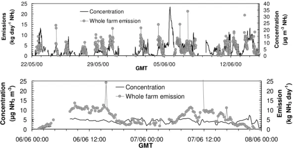
from 0 to 0.5 kg h−1 NH3. Figure 4 shows a clear diurnal
variation with a maximum emission at midday and a mini-mum during the night. This daily variability is not always due to concentration changes, as shown in Fig. 4 (bottom graph) where concentration difference χ–χbgd is constant and the source strength varies. The variability is also due to the turbulent diffusivity increasing during the day, therefore requiring a larger source to generate a similar concentration at a given distance. Averaging the inferred hourly emission rates over all the available data (for westerly winds), and con-verting to daily emission rates lead to an average emission of 6.4 kg d−1NH3, with a standard error of 0.18 kg d−1 NH3
(N=495).
The inferred emission strength was averaged to hourly val-ues in order to estimate a mean daily pattern (Fig. 5). The daily pattern was observed throughout the period, with a min-imum between 01:00 and 02:00 GMT in the morning and a maximum between 07:00 and 09:00 GMT in the morn-ing, then decreasing towards the end of the day. This pat-tern is partly reflected by the concentration difference be-tween Site 3 and the background concentration, also shown in Fig. 5. Note that there are not many data at night, due tou∗
or|L|being below the model requirement under stable con-ditions, so that the results obtained for night-time conditions are based on less data than for the day.
5 Discussion
5.1 Emissions from the farm buildings estimated with different techniques and sensitivity analysis
The averaged daily emission estimated with the Gaussian-3D model was found to be 9.2±0.7 kg d−1 NH3, and
6.4±0.18 kg d−1NH3(±standard errors) with the Huang-3D
model, while it was estimated as 9.6 kg d−1 NH3 with the
emission factors approach. The inferred emission strength with the Gaussian-3D and the Huang-3D model would rep-resent 3.3 t NH3year−1and 2.3 t NH3year−1, respectively.
Although, the inventory emission factors do not include for-mal uncertainty estimates, the comparison with the esti-mates of Demmers et al. (2001) for dairy cattle of 8.9 kg NH3 animal−1yr−1compared with 10.35 kg animal−1yr−1
0 5 10 15 20 25 30 35 40 NH 3 (µ g m
-3 )
bkg+modelruns NH3 bkg Measured
AM1 0 5 10 15 20 25 30 35 40 NH
3 (µ
g
m
-3 )
AM2 0 5 10 15 20 25 30 35 40 NH
3 (µ
g m -3 ) AM3 0 10 20 30 40 50 60 70 80 90 100 20-05 21-05 22-05 23-05 24-05 25-05 26-05 27-05 28-05 29-05 30-05 31-05 01-06 02-06 03-06 04-06 05-06 06-06 07-06 08-06 09-06 10-06 11-06 12-06 13-06 14-06 15-06 16-06 17-06 S our c e s tr engt h k gN H 3 /day AM3 AM1 AM2 0 5 10 15 20 25 30 35 40 NH 3 (µ g m
-3 )
bkg+modelruns NH3 bkg Measured
AM1 0 5 10 15 20 25 30 35 40 NH
3 (µ
g
m
-3 )
AM2 0 5 10 15 20 25 30 35 40 NH
3 (µ
g m -3 ) AM3 0 10 20 30 40 50 60 70 80 90 100 20-05 21-05 22-05 23-05 24-05 25-05 26-05 27-05 28-05 29-05 30-05 31-05 01-06 02-06 03-06 04-06 05-06 06-06 07-06 08-06 09-06 10-06 11-06 12-06 13-06 14-06 15-06 16-06 17-06 S our c e s tr engt h k gN H 3 /day AM3 AM1 AM2
Fig. 3.Example of measured and modelled concentration with the Gaussian-3D model by AM1-3 at Site 3. The source-strengths of the farm buildings were estimated by minimizing the difference between the measured and the modelled concentrations at all locations.
In order to better understand the uncertainty in the differ-ent emission estimates a sensitivity analyses was done. The result of this exercise is summarized in Table 6 with the ma-jor parameters that might affect the estimation of the emis-sion strength using the two models 3-D disperemis-sion models, as well as the effect of taking into account dry deposition downwind of the source using FIDES-2D.
It can be seen that the Huang-3D and the FIDES-2D mod-els are sensitive to the height of the source and the roughness length with a maximum error around 20%. The Gaussian-3D model calculation showed a similar result for thezochange
from 0.1–1. The Gaussian-3D model uses differentzovalues
per source with larger values for stables at the back of the fram. A change of 50% of all these values had a 10% effect on the average emission level.
The difference in source height, already mentioned above, can have a 20% effect for the Huang-3D model with a lower emission estimates when the source height increases. This will bring the Huang-3D model and the Gaussian-3D model closer together. The source height range in Table 6 only shows a small (2%) effect on the Gaussian-3D model esti-mate. Only when changing the source height further for ex-ample from 4 to 10 m this model would decrease the emis-sion estimate by 8%. For the Gaussian-3D model changing the stability classification at a 15 min interval from Pasquill class D neutral to C or E would increase or decrease the emis-sion estimate by 40% respectively. Furthermore, changing the initial dispersion in the wake of the buildings from 5 m to 10 m reduced the emission by 20%.
0 5 10 15 20 25
22/05/00 29/05/00 05/06/00 12/06/00
GMT
E
m
is
si
o
n
s
(k
g day
-1 NH
3
)
0 5 10 15 20 25 30 35 40
C
oncent
rat
io
n
(µ
g
m
-3 NH
3
)
Concentration
Whole farm emission
0 5 10 15 20 25
06/06 00:00 06/06 12:00 07/06 00:00 07/06 12:00 08/06 00:00
GMT
C
onc
e
n
tr
a
tion
(µ
g
N
H3
m
-3 )
0 5 10 15 20 25
E
m
issi
o
n
(k
g
N
H3
da
y
-1 )
Concentration Whole farm emission
Fig. 4.Top graph: time course of the NH3emission strength as inferred with the Huang-3D model using the averaged concentration measured
for the wind direction 240◦–300◦at Site 3 and the background concentration measured at Site 6. Also shown is the concentration difference Site 3–Site 6. Bottom graph: magnification for the period 6–8 June.
Table 5. Ammonia source-strength estimated with the Gaussian-3D model, as compared to that estimated from the emission factors of D¨ohler et al. (2002). The total amount of ammonia emitted per year estimated using the Gaussian-3D model is 3.3×10³kg year−1NH3as compared to the inventory estimate of 3.5×10³kg year−1NH3. These values correspond to averaged daily emissions of 9.2 kg d−1NH3and
9.6 kg d−1NH3, respectively.
Estimated from emission factors (D¨ohler et al., 2002) Estimated with the AMANDA measurements (Site 3) and Gaussian model (this study) Building Animals Number of animals Emission per building Percentage contribution Emission per building Percentage contribution
(Fig. 1) kg NH3year−1 % kg NH3year−1 %
A Cattle 60 621 18% 0 0%
B Cattle 60 621 18% 729 22%
C Cattle 11 114 3% 559 17%
D Cattle 48 497 14% 598 18%
E Bulls 64 249 7% 0 0%
F Cattle 80 828 24% 4 0%
G Calves 60 233 7% 0 0%
H Calves 0 0 0% 0 0%
I Pigs 80 158 5% 926 28%
J Pigs 45 89 3% 43 1%
K Pigs 45 89 3% 483 14%
Total 3.5×10³ 100% 3.3×10³ 100%
151% increase for a 400 m source). The measured NH3
con-centration at 230 m downwind from the farm will be lowered by the dry deposition taking place between the farm build-ings and Site 3. This was studied with the FIDES-2D model and the effect was in the order of 40%. When correcting both the Gauss model and the Huang 3-D model, the latter will be close to the emission inventory result and the Gauss model estimate will be above that level.
Neglecting the deposition issue for the Gauss model, the different sensitivity runs provide a set of emission estimates that have a standard deviation of 25% around the emission level of 9.2 kg NH3 d−1. This uncertainty range is
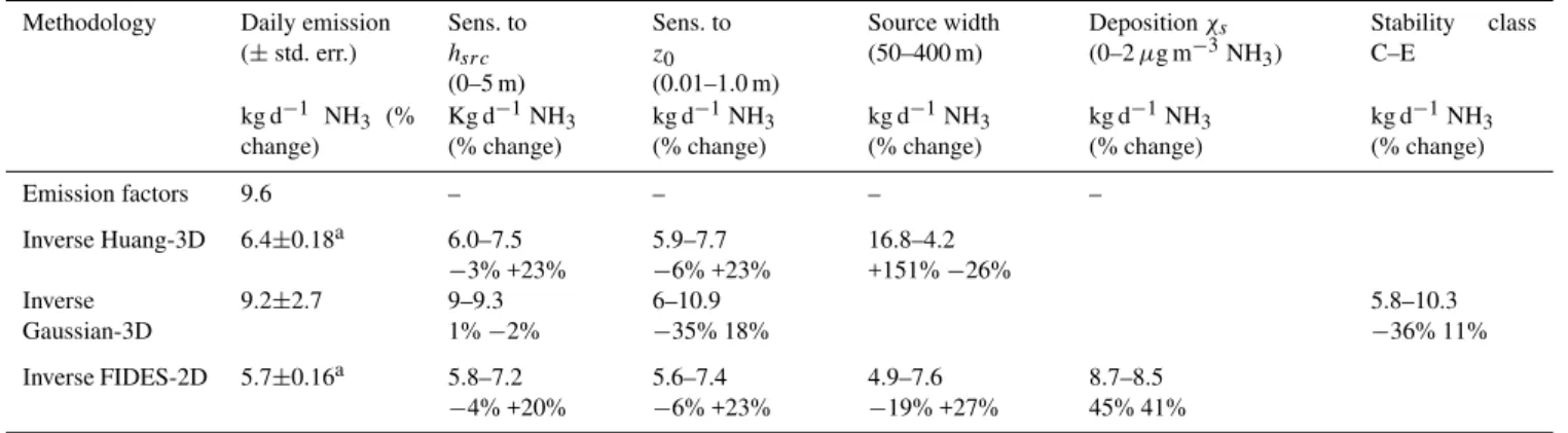
Table 6.Daily emission of the source estimated using the emission factor and the modelling approach, and sensitivity of each estimate to micrometeorological parameters. Standard parameters used were:zsrc=1.0 m,z0=0.10 m, source width = 180 m, and no dry deposition. In
the sensitivity analysis,hsrchave been set to 0 and 5 m height,z0has been set to 0.01 m and 1.0 m, the source width has been set to 50 and
400 m, and in the deposition sensitivity analysis, the stomatal compensation pointχs has been set to 0 and 1µg m−3NH3. The cuticular Rw and stomatal resistanceRs were estimated asRw=7 exp((100−RH)/12), andRs=30×{1+200/max(0.01, St)}, where RH is the relative
humidity atz′0and St is the global solar radiation.
Methodology Daily emission (±std. err.)
Sens. to
hsrc
(0–5 m)
Sens. to
z0
(0.01–1.0 m)
Source width (50–400 m)
Depositionχs
(0–2µg m−3NH3)
Stability class C–E
kg d−1 NH3 (% change)
Kg d−1NH3 (% change)
kg d−1NH3 (% change)
kg d−1NH3 (% change)
kg d−1NH3 (% change)
kg d−1NH3 (% change)
Emission factors 9.6 – – – –
Inverse Huang-3D 6.4±0.18a 6.0–7.5 −3% +23%
5.9–7.7 −6% +23%
16.8–4.2 +151%−26% Inverse
Gaussian-3D
9.2±2.7 9–9.3 1%−2%
6–10.9 −35% 18%
5.8–10.3 −36% 11%
Inverse FIDES-2D 5.7±0.16a 5.8–7.2 −4% +20%
5.6–7.4 −6% +23%
4.9–7.6 −19% +27%
8.7–8.5 45% 41%
astandard error estimated with 632 data.
0 200 400 600 800 1000
0:00 4:00 8:00 12:00 16:00 20:00 0:00
GMT
Emission strength
(g NH
3
ho
ur
-1)
0 2 4 6 8 10
Concentration difference
(µ
g NH
3
m
-3) Srce strength mean
C - Cbgd
Fig. 5.Diurnal variability of the farm NH3source strength as
esti-mated with the Huang-3D model for a wind sector of 240◦–300◦. The concentration difference between Site 3 and the background at Site 6 (C–Cbgd)is also given. The dark circles represent the source
strength during the whole period that has been hourly averaged to give the mean source strength for each hour. The error bars are the standard errors.
along a vertical profile up to about 10 m height would have provided better constraints on the parameters that set the ver-tical dispersion in the model.
The analysis shows that deposition as well as the source geometry can really influence the emission strength inferred with inverse modeling techniques. However of these two effects, deposition is probably the more problematic in the case of emissions from farm building, since there is a much larger uncertainty on the deposition parameters (Rs and
par-ticularlyRw andχs)than on the source geometry. Indeed,
the fields in between the source and Site 3 were patches of small crop trials of varyingRs,Rw andχs, which makes it
difficult to define a unique surface characteristic. Moreover,
Rw is a very uncertain parameter that has a major influence
on local deposition (Flechard et al., 1999; Loubet and Cellier, 2002; Burkhardt et al., 2009). This constitutes a major uncer-tainty in the dispersion model approach, which is difficult to overcome. One way would be to perform the measurements closer to the source and at higher levels (such as Welch et al., 2005b). However close to the farm, the influence of the farm buildings on the flow would prohibit the use of Gaussian-like models, and would require more sophisticated approaches. This study also suggests that the used of a 3-D model relies on a precise description of the size of the source.
Finally, apart from the model uncertainties there are ad-ditional possibilities that can cause a difference between the emission factor calculation and the model result:
1. The small sampling time due to the concentration mea-surements being done only on the east of the farm, which may hence induce a bias if wind directions show a daily pattern. This was indeed the case, for the west sector at 15:00 there are 4 times more datapoints avail-able compared with 05:00. However, this would have lead to a bias toward higher emission estimates. 2. The experimental farm seemed especially well
0 50 100 150 200 250 300 350 400 450 500
14 16 18 20 22 24
Indoor temperature (°C)
Em
issio
n
st
reng
th
(g
NH3 ho
ur-1)
× ±
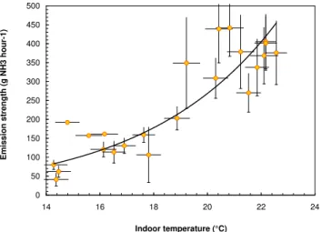
Fig. 6. Hourly averaged emission strength for a wind sector of 240◦–300◦as a function of hourly mean indoor temperature (mea-sured for the main cattle building A). The bold line is a regression with equation: Source [g h−1 NH3]=2.03 exp(0.2342×T [◦C]), R2=0.771. The error-bars are±standard deviation.
In literature the underestimation of emissions by the disper-sion models has been observed before. For example, Welch et al. (2005b) found a collection efficiency of 80% using the ADMS model in a controlled NH3release experiment.
How-ever, Flesch et al. (2004) found a much better collection effi-ciency with a methane tracer using a backward Lagrangian Stochastic model under flat terrain conditions. Flesch et al. (2004) also showed that the modelling approach was not reliable under strongly stratified conditions. Michorius et al. (1997) evaluated that the underestimation of NH3
emis-sion by a farm building using a Gaussian-3D approach and concentrations measured at 100 m varied from 47% to 68% of the expected emission.
5.2 Daily variability of the emissions from a naturally ventilated building
Figures 4 and 5 show that the emission strength followed a clear diurnal pattern, with a maximum in mid-morning and a minimum at night. Although some of this variability is re-flected in the concentration change (Fig. 5), this is not always the case, because of the daily pattern of the turbulent diffusiv-ity. The question arises whether this variability in emission is real or is a bias linked with the inference method. Indeed, the emission from farm houses with forced ventilating sys-tems can be rather constant with time, due to a rather con-stant indoor temperature regulated by the ventilation system. However, at the FAL farm studied here, most of the buildings are naturally ventilated, which implies that the indoor tem-peratures fluctuate and that the flow rate through the build-ings also changes with environmental conditions (Welch et al., 2005b; Zhang et al., 2005). This seems to be confirmed by Fig. 5, where one can see a morning maximum, which
0 200 400 600 800
Emissio
n
stre
ngth
(g
N
H
3
hour
-1
)
0.3 0.4 0.5 0.6 0.7 0.8 0.9 1.0
Co
nvectio
n ve
clocity
(m
m
s-1)
Srce strength mean Free convection veclocity Forced convection velocity (a)
0 200 400 600 800
0:00 4:00 8:00 12:00 16:00 20:00 0:00
GMT
Emi
s
si
o
n
st
ren
g
th
(g
NH3 ho
ur-1
)
0.9 1.1 1.3 1.5 1.7 1.9
Co
nv
ec
ti
on
ve
lo
ci
ty
(mm
s-1)
Srce strength mean
Modelled convection velocity (b)
± Fig. 7. Hourly averaged emission strength for a wind sector of 240◦–300◦,(a)free and forced convection velocities calculated as 1/Rb, and(b)resultant total convection velocity (sum of free and
forced convection velocities). The error-bars are±standard errors. A linear regression between the convection velocity and the emis-sion strength gives anR2=0.97.
might for example be due to a flushing out of NH3
accumu-lated during the night.
Figure 6 shows the hourly-mean emission strength as a function of the indoor temperature of the main cattle building (A in Fig. 1). This suggests that the inferred daily variability of the emission strength is real, since NH3 emission is
ex-pected to vary as the exponential function of the temperature according to the Clausius-Clapeyron law (e.g., with a dou-bling of emission for every 5◦C increase, Sutton et al., 2001). This dependence of NH3 emissions to indoor temperature
was experimentally demonstrated by Zhang et al. (2005) over a range of temperature 5–23◦C. However Zhang et al. found a maximum increase by a factor of 3 over the range of tem-perature observed here (14–23◦C), whereas Fig. 6 shows an
increase of up to a factor of 7. On the basis of the solubil-ity equilibria, a factor 4 increase would have been expected. This suggests that the response of Fig. 6 may include ef-fects of temperature as well as correlated efef-fects linked with changes in the ventilation rate.
velocity were calculated by adapting Monteith and Unsworth (1990) and Murphy et al. (1977) approaches, respectively. These velocities were computed as the inverse of the transfer resistanceRb, usingu∗as a velocity scale, the difference
be-tween indoor and outdoor temperatures, and a characteristic size of the building of 10 m was taken. Although the expres-sions from Murphy et al. (1977) are not adapted to free and forced convection in buildings, they can give a good quali-tative information on the daily variability of the ventilation rate. They are shown in Fig. 7, calculated from hourly aver-ages, along with the source strength, and the resultant con-vective velocity (the sum of the two). The daily pattern of free convection (Fig. 7a) shows two maxima, one between 4h and 8h, and the other around 22 h. This pattern is due to a time de-correlation between the indoor and the outdoor tem-peratures, which might be explained by the building being heated more rapidly than the air in the morning (because of the solar radiation onto the roof and small ventilation), and a longer decrease at night due to the naturally forced ventila-tion being small at that time. On the opposite, the modelled forced convection velocity follows directly the daily pattern ofu∗.
It can be seen that the resultant convective velocity fol-lows the source strength pattern very well (Fig. 7a). A linear regression between the convective velocity and the emission strength gives anR2=0.67. This suggests that the emission pattern observed in Fig. 5 is probably caused by (i) the in-door concentration increasing with inin-door temperature, as suggested by Fig. 6, and (ii) the ventilation rate increasing also during the day as resulting from the combination of nat-ural convection (indoor temperature change), and forced con-vection (external wind).
6 Conclusions
Within the framework of the European GRAMINAE project, an intensive joint field experiment was performed at the FAL research station in Braunschweig (Germany), during May and June 2000. This experiment, summarized in Sutton et al. (2009b) has brought together many atmospheric NH3
con-centration measurements techniques located at several sites around a cluster of farm buildings. This gave a great op-portunity to use the measured NH3concentration, as well as
mobile fast sensor measurements to infer the emission from the farm building with inverse modelling technique. Three models were used, a Gaussian-3D plume model, the local dispersion model of Huang (1979), and the FIDES-2D model to account for NH3deposition downwind from the source.
The inferred emission strength was on average 6.4 kg d−1 NH3 for the Huang-3D model and 9.2±0.7 kg d−1NH3 for
the Gaussian-3D plume model. The mobile NH3
measure-ments provided valuable data on the horizontal dispersion of the NH3plume form the farm houses. These data were used
to constrain the dispersion model parameters. Concentration
measurements of the vertical distribution of NH3that could
be used to evaluate the vertical dispersion of the NH3plume
were not available but are recommended for similar experi-ments in future.
A sensitivity analysis showed that the inference method was very sensitive to the deposition scheme used, and when a maximum deposition was applied, the farm emission strength could be increased by 45%. The height and size of the source, the surface roughness, the Pasquill stability classes were found to influence the emission strength estimates both with the Huang-3D and the Gauss model by up to 50%. The source-strength exhibited a clear diurnal cycle with a maxi-mum in the morning (07:00–08:00 GMT) and a minimaxi-mum at night. This variability can be fully explained by changes in the indoor temperature and the ventilation rate.
In the context of remaining uncertainty in the inventory es-timates and lack of independent measurement of NH3
emis-sions from the buildings, the present work does not fully val-idate the approach used. However, the application of disper-sion models combined with NH3 concentrations measured
at large distances downwind, provides an approach in close agreement with the inventory, while this study demonstrates the need to consider other interacting factors, such as dry de-position between the source and the measurement location.
Acknowledgements. The work presented here was partly funded by the EU FP5 GRAMINAE Project (EU contract ENV4-CT98-0722). Final synthesis of this paper was conducted as part of the NitroEurope Integrated Project We thank the Spanish Commission of Advanced Education and Scientific Research (Direcci´on General de Ense˜nanza Superior e Investigaci´on Cient´ıfica) who provided funding for J. Mosquera to come to the Energy Research Center of the Netherlands (ECN) as a postdoctoral fellow, and the UK Department for Environment Food and Rural Affairs (Defra).
Edited by: J. K. Schjoerring
References
Asman, W. A. H.: Ammonia emission in Europe: updated emission and emission variations, Report 228471008, National Institute of Public Health and Environmental Protection (RIVM), Bilthoven, The Netherlands, 1992.
Bobbink, R., Boxman, D., Fremstad, E., Heil, G., Houdijk, A., and Roelofs, J.: Critical loads for nitrogen eutrophication of terres-trial and wetland ecosystems based upon changes in vegetation and fauna, in: Critical loads for nitrogen, edited by: Grennfelt, P. and Th¨ornel¨of, E., 41 p., Nordic Council of Ministers, Copen-hagen, 1992.
Bouwman, A. F., Lee, D. S., Asman, W. A. H., Dentener, J. F., van de Hoek, K. W., and Olivier, J. J. G.: A global emission inventory for ammonia, Global Biogeochemical Cycles, 11, 561– 587, 1997.
grassland canopy, Biogeosciences, 6, 67–83, 2009, http://www.biogeosciences.net/6/67/2009/.
Bussink, D. W. and Oenema, O.: Ammonia volatilization from dairy farming systems in temperate areas: a review, Nutrient Cy-cling in Agroecosystems, 51, 1352–2310, 1998.
Demmers, T. G. M., Burgess, L. R., Short, J. L., Phillips, V. R., Clark, J. A., and Wathes, C. M.: Ammonia emissions from two mechanically ventilated UK livestock buildings, Atmos. Envi-ron., 33, 107–116, 1999.
D¨ohler, H., D¨ammgen, U., Berg, W., Bergschmidt, A., Brunsch, R., Eurich-Menden, B., L¨uttich, M., and Osterburg, B.: Adaptation of the German emission calculation methodology to international guidelines, determination and forecasting of ammonia emissions from German agriculture, and scenarios for reducing them by 2010, Umweltbundesamt (Berlin), Forschungsbericht 299, UBA FB000249, 2002 (in German, summary in English).
Dore, C. J., Jones, B. M. R., Scholtens, R., Huis in’T Veld, J. W. H., Burgess, L. R., and Phillips, V. R.: Measuring ammonia emission rates from livestock buildings and manure stores – Part 2: Com-parative demonstrations of three methods on the farm, Atmos. Environ., 38, 3017–3024. 2004.
Erisman, J. W., Otjes, R., Hensen, A., Jongejan, P., v. d. Bulk, P., Khlystov, A., Mols, H., and Slanina, S.: Instrument development and application in studies and monitoring of ambient ammonia, Atmos. Environ., 35, 1913–1922, 2001.
Flesch, T. K., Wilson, J. D., Harper, L. A., and Crenna, B. P.: Es-timating gas emissions from a farm with an inverse-dispersion technique, Atmos. Environ., 39, 4863–4874, 2005.
Flechard, C., Fowler, D., Sutton, M. A., and Cape, J. N.: A dy-namic chemical model of bi-directional ammonia exchange be-tween semi-natural vegetation and the atmosphere, Q. J. Roy. Meteorol. Soc., 125, 2611–2641, 1999.
Flesch, T. K., Wilson, J. D., Harper, L. A., Todd, R. W., and Cole, N. A.: Determining ammonia emissions from a cattle feedlot with an inverse dispersion technique, Agric. For. Meteorol., 144, 139– 155, 2007.
Galloway, J. N.: Acid deposition: perspectives in time and space. Water, Air Soil Pollut., 85, 15–24, 1995.
Gash, J. H. C.: A note on estimating the effect of a limited fetch on micrometeorological evaporation measurements, Bound. Lay. Meteorol., 35, 409–413, 1985.
Heij, G. J. and Schneider, T. (Eds.): Acidification research in the Netherlands, pp. 3–24, Studies in Environmental Science 46, El-sevier, Amsterdam, 1991.
Heij, G. J. and Schneider, T. (Eds.): Dutch Priority Programme on Acidification. Final report No. 300-05, National Institute of Pub-lic Health and Environmental Protection (RIVM), Bilthoven, The Netherlands, 1995.
Hensen, A. and Scharff, H.: Methane emission estimates from land-fills obtained with dynamic plume measurements, Water, Air Soil Pollut., Kluwer, focus, 1, 455–464, 2001.
Huang, C. H.: A theory of dispersion in turbulent shear flow, Atmos. Environ., 13, 453–463, 1979.
Jarvis, S. C. and Pain, B. F.: Ammonia volatilisation from agricul-tural land. Proceedings of the Fertiliser Society 298, 35 pp., The Fertiliser Society, Peterborough, 1990.
Lin, J. S. and Hildemann, L. M.: A Generalized mathematical scheme to analytically solve the atmospheric diffusion equation with dry deposition, Atmos. Environ., 31, 59–71, 1997.
Loubet, B. and Cellier, P.: Experimental assessment of atmospheric ammonia dispersion and short-range dry deposition in a maize canopy, Water Air Soil Pollut., 1(5/6), 157–166, 2002.
Loubet, B., Cellier, P., Milford, C., and Sutton, M. A.: A coupled dispersion and exchange model for short-range dry deposition of atmospheric ammonia, Q. J. Roy. Meteorol. Soc., 132, 1733– 1763, 2006.
Loubet, B., Milford, C., Sutton, M. A., and Cellier, P.: Investiga-tion of the interacInvestiga-tion between sources and sinks of atmospheric ammonia in an upland landscape using a simplified dispersion-exchange model, J. Geophys. Res., 106(D20), 24183–24196, 2001.
Michorius, J. A. T., Hartog, K. D., Scholtens, R., and Harssema, H.: Measuring ammonia emissions from building complexes using the flux frame method and the Gaussian plume model: a feasibil-ity study, Translation – Silsoe Research Institute, 1997. Milford, C., Theobald, M. R., Nemitz, E., Hargreaves, K. J.,
Hor-vath, L., Raso, J., D¨ammgen, U., Neftel, A., Jones, S. K., Hensen, A., Loubet, B., Cellier, P., and Sutton, M. A.: Ammo-nia fluxes in relation to cutting and fertilization of an intensively managed grassland derived from an inter-comparison of gradient measurements, Biogeosciences, 6, 819–834, 2009,
http://www.biogeosciences.net/6/819/2009/.
Monteith, J. L. and Unsworth, M. H.: Principles of Environmental Physics, 2nd ed., 291 pp., Arnold, New York, 1990.
Mosquera, J., Monteny, G. J., and Erisman, J. W.: Overview and assessment of techniques to measure ammonia emissions from animal houses: the case of the Netherlands, Environ. Pollut., 135, 381–388, 2005.
Nemitz, E., Hargreaves, K. J., Neftel, A., Loubet, B., Cellier, P., Dorsey, J. R., Flynn, M., Hensen, A., Weidinger, T., Meszaros, R., Horvath, L., Dmmgen, U., Fr¨uhauf, C., L¨opmeier, F. J., Gallagher, M. W., and Sutton, M. A.: Intercomparison and as-sessment of turbulent and physiological exchange parameters of grassland, Biogeosciences, 6, 1445–1466, 2009,
http://www.biogeosciences.net/6/1445/2009/.
Pasquill, F.: Atmospheric Diffusion, 2nd ed., J. Wiley & Sons, New York, 1974.
Pain, B. F., van der Weerden, T. J., Chambers, B. J., Phillips, V. R., and Jarvis, S. C.: A new inventory for ammonia emissions from UK agriculture, Atmos. Environ., 32, 309–313, 1998.
Philip, J. R.: The theory of local advection: 1, J. Meteorol., 16, 535–547, 1959.
Phillips, V. R., Lee, D. S., Scholtens, R., Garland, J. A., and Sneath, R. W.: A review of methods for measuring emission rates of ammonia from livestock buildings and slurry or manure stores, part 2: monitoring flux rates, concentrations and airflow rates, J. Agricult. Eng. Res., 78, 1–14, 2001.
Raupach, M. R.: Stand overstorey processes, Philos. Trans. R. Soc. London, Ser. B, 324, 175–190, 1989.
Scholtens, R., Dore, C. J., Jones, B. M. R., Lee, D. S., and Phillips, V. R.: Measuring ammonia emission rates from livestock build-ings and manure stores – Part 1: Development and validation of external tracer ratio, internal tracer ratio and passive flux sam-pling methods, Atmos. Environ., 38, 3003–3015, 2004. Smith, F. B.: The diffusion of smoke from a continuous elevated
point source into a turbulent atmosphere, J. Fluid Mech., 2, 49– 76, 1957.
of the backwards Lagrangian stochastic dispersion technique for measuring ammonia emission from small field-plots, European J. Agronomy, 23, 1–7, 2005.
Sutton, O. G.: A theory of eddy diffusion in the atmosphere, Proc. R. Soc. A, 135, 143–165, 1932.
Sutton, M. A., Nemitz, E., Theobald, M. R., Milford, C., Dorsey, J. R., Gallagher, M. W., Hensen, A., Jongejan, P. A. C., Erisman, J. W., Mattsson, M., Schjoerring, J. K., Cellier, P., Loubet, B., Roche, R., Neftel, A., Hermann, B., Jones, S. K., Lehman, B. E., Horvath, L., Weidinger, T., Rajkai, K., Burkhardt, J., L¨opmeier, F. J., and Daemmgen, U.: Dynamics of ammonia exchange with cut grassland: strategy and implementation of the GRAMINAE Integrated Experiment, Biogeosciences, 6, 309–331, 2009a, http://www.biogeosciences.net/6/309/2009/.
Sutton, M. A., Nemitz, E., Milford, C., Campbell, C., Erisman, J. W., Hensen, A., Cellier, P., David, M., Loubet, B., Personne, E., Schjoerring, J. K., Mattsson, M., Dorsey, J. R., Gallagher, M. W., Horvath, L., Weidinger, T., Meszaros, R., D¨ammgen, U., Neftel, A., Herrmann, B., Lehman, B. E., Flechard, C., and Burkhardt, J.: Dynamics of ammonia exchange with cut grassland: synthesis of results and conclusions of the GRAMINAE Integrated Exper-iment, Biogeosciences Discuss., 6, 1121–1184, 2009b,
http://www.biogeosciences-discuss.net/6/1121/2009/.
Thomson, D. J.: Criteria for the selection of stochastic models of particle trajectories in turbulent flows, J. Fluid Mech., 180, 529– 556, 1987.
Van Breemen, N., Burrough, P. A., Velthorst, E. J., van Dobben, H. F., de Wit, T., Ridder, T. B., and Reijnders, H. F. R.: Soil acid-ification from ammonium sulphate in forest canopy throughfall, Nature, 288, 548–550, 1982.
Welch, D. C., Colls, J. J., Demmers, T. G. M., and Wathes, C. M. A.: Methodology for the measurement of distributed agricultural sources of ammonia outdoors – Part 1: validation in a controlled environment, Atmos. Environ., 39, 663–672, 2005a.
Welch, D. C., Colls, J. J., Demmers, T. G. M., and Wathes, C. M.: A methodology for the measurement of distributed agricultural sources of ammonia outdoors – Part 2: Field validation and farm measurements, Atmos. Environ., 39, 673–684, 2005b.
Wilson, J. D., Thurtell, G. W., Kidd, G. E., and Beauchamp, E. G.: Estimation of the rate of gaseous mass transfer from a surface source plot to the atmosphere, Atmos. Environ., 16, 1861–1867, 1982.
Wyers, G. P., Otjes, R. P., and Slanina, J.: A continuous-flow denuder for the measurement of ambient concentrations and surface-exchange fluxes of ammonia, Atmos. Environ., 27A(13), 2085–2090, 1993.
Yeh, G. T. and Huang, C. H.: Three-dimensional air pollutant mod-eling in the lower atmosphere, Bound. Lay. Meteorol., 9, 381– 390, 1975.