SURFATM-NH<sub>3</sub>: a model combining the surface energy balance and bi-directional exchanges of ammonia applied at the field scale

(1)

BGD

6, 71–114, 2009

Bi-directional exchanges of ammonia – the

SURFATM-NH₃ model

E. Personne et al.

Title Page

Abstract Introduction

Conclusions References

Tables Figures

◭ ◮

Back Close

Full Screen / Esc

Printer-friendly Version

Interactive Discussion Biogeosciences Discuss., 6, 71–114, 2009

www.biogeosciences-discuss.net/6/71/2009/ © Author(s) 2009. This work is distributed under the Creative Commons Attribution 3.0 License.

Biogeosciences Discussions

Biogeosciences Discussionsis the access reviewed discussion forum ofBiogeosciences

SURFATM-NH

₃

: a model combining the

surface energy balance and bi-directional

exchanges of ammonia applied at the

field scale

E. Personne1, B. Loubet1, B. Herrmann2, M. Mattsson3, J. K. Schjoerring3, E. Nemitz4, M. A. Sutton4, and P. Cellier1

1

UMR Environment et Grandes Cultures/INRA – AgroParisTech, 78 850 Thiverval Grignon, France

2

Agroscope Reckenholz-T ¨anikon Research Station ART, Reckenholzstrasse 191, 8046 Z ¨urich, Switzerland

3

Plant and Soil Science Laboratory, University of Copenhagen, Faculty of Life Sciences, Thorvaldsensvej 40, 1871 Frederiksberg C, Copenhagen, Denmark

4

Centre for Ecology and Hydrology, Edinburgh Research Station, Bush Estate, Penicuik, Midlothian, EH26 0QB, UK

Received: 30 September 2008 – Accepted: 23 October 2008 – Published: 6 January 2009 Correspondence to: E. Personne (erwan@bcgn.grignon.inra.fr)

(2)

BGD

6, 71–114, 2009

E. Personne et al.

Title Page

Tables Figures

◭ ◮

Back Close

Full Screen / Esc

Interactive Discussion Abstract

A new biophysical model SURFATM-NH3, simulating the ammonia (NH3) exchange

between terrestrial ecosystems and the atmosphere is presented. SURFATM-NH3

consists of two coupled models: (i) an energy budget model and (ii) a pollutant ex-change model, which distinguish the soil and plant exex-change processes. The model

5

describes the exchanges in terms of adsorption to leaf cuticles and bi-directional trans-port through leaf stomata and soil. The results of the model are compared with the flux measurements over grassland during the GRAMINAE Integrated Experiment at Braunschweig, Germany. The dataset of GRAMINAE allows the model to be tested in various climatic and agronomic conditions: prior to cutting, after cutting and then

10

after the application of mineral fertilizer. The whole comparison shows close agree-ment between model and measureagree-ments for energy budget and ammonia fluxes. The major controls on the soil and plant emission potential are the physicochemical pa-rameters for liquid-gas exchanges which are integrated in the compensation points for live leaves, litter and the soil surface. Modelled fluxes are highly sensitive to soil and

15

plant surface temperatures, highlighting the importance of accurate estimates of these terms. The model suggests that the net flux depends not only on the foliar (stomatal) compensation point but also that of leaf litter. SURFATM-NH3 represents a

compre-hensive approach to studying pollutant exchanges and its link with plant and soil func-tioning. It also provides a simplified generalised approach (SVAT model) applicable for

20

atmospheric transport models.

1 Introduction

The exchange of trace gases and vapour pressure between terrestrial ecosystem and atmosphere is a key process the Earth’s Biosphere functioning: at the local, regional and global scale, these exchanges participate in element cycling, influencing

ecosys-25

(3)

BGD

6, 71–114, 2009

E. Personne et al.

Title Page

Tables Figures

◭ ◮

Back Close

Full Screen / Esc

Interactive Discussion of trace gases (e.g., NH₃, O₃, SO₂, N₂O) at the surface is often included in mesoscale

transport models or global scale models using a dry deposition velocity approach (Fowler et al., 1989; Wesely, 1989; Tulet et al., 2000) or emission factors (Li et al., 2001; Freibauer, 2003; Hyde et al., 2003), although recent studies use improved pro-cess based models (Grunhage and Haenel, 1997; Polcher et al., 1998; Ganzeveld et

5

al., 2002; Nikolov and Zeller, 2003; Pinder et al., 2004; Theobald et al., 2004). In this context, this paper concentrates on atmospheric ammonia (NH₃) as a reference pollutant for the conception of exchange schemes of soil-plant-atmosphere interface that can be integrated at the lower-boundary conditions in global scale models or in mesoscale transport models.

10

Indeed, atmospheric ammonia (NH₃) mainly originates from agriculture (Bouwman et al., 1997; Anderson et al., 2003; Sutton et al., 2007; Zhang et al., 2008), of which animal waste is the main source (Van der Hoek, 1998; Zhang et al., 2008). Ammonia deposition leads to acidification and eutrophication of semi-natural ecosystems (Van Breemen and Van Dijk, 1988; Fangmeier et al., 1994; Dragosits et al., 2002) and to

15

decrease of the plant biodiversity (Bobbink, 1991; Krupa, 2003; Stevens et al., 2004, 2006). The concentrations of NH₃ in the environment are generally in the range 0.1 to 5 µg m−3 NH3 and can reach several tens of µg m−

3

NH3 in the vicinity of strong

sources (Sutton et al., 1998b; Loubet et al., 2001). As a major constituent of the plant metabolism, NH3 can either be absorbed or emitted by the vegetation (Sutton et al., 20

1993; Schjoerring et al., 2000). The bi-directional nature of NH3 exchange between

the atmosphere and the surface has been demonstrated in many studies (Farquhar et al., 1980; Erisman and Wyers, 1993; Sutton et al., 1995, 1998a).

However, the NH3flux above a canopy results from the combination of sources and

sinks within the canopy, as emphasised by Nemitz et al. (2000a). In a grassland canopy

25

the litter may be a strong source of NH₃ as suggested by laboratory studies (Husted and Schjoerring, 1995; Mattsson and Schjoerring, 2002, 2003), but the stomata could also release NH3following fertilisation (Husted et al., 2000; Loubet et al., 2002).

(4)

BGD

6, 71–114, 2009

E. Personne et al.

Title Page

Tables Figures

◭ ◮

Back Close

Full Screen / Esc

Interactive Discussion Modelling NH3exchange has proven to be a good mean to interpret measured NH3

fluxes at the canopy scale, and especially to evaluate the contribution of each canopy compartment to the net flux (e.g. Nemitz et al., 2000b). However, NH3emissions from

the ground surface or from plants is known to depend exponentially on temperature, due to thermodynamic equilibria (e.g. Schjoerring, 1997), and stomatal resistance as

5

any other gases (Sutton et al., 1993). Hence the NH3 exchange model needs to

cor-rectly simulate the surface temperature of emitting or absorbing compartments (stom-ata and litter/soil surface) as well as the stom(stom-atal resistance.

In this paper, we present a bi-directional two-layer resistance model for heat and NH3, parameterised for a grassland canopy. The model SURFATM-NH3 combines 10

a resistive approach for the energy balance and for the NH₃exchange. It incorporates an NH3stomatal compensation point as well as a litter or soil NH3compensation point,

and a cuticular pathway. SURFATM-NH3 model is then evaluated against measured

fluxes of energy, water and ammonia, during the GRAMINAE Integrated Experiment above managed grassland at Braunschweig, Germany (Sutton et al., 2008).

15

2 Model description

SURFATM-NH₃ is a one-dimensional, bi-directional model, which simulates the latent (λE) and sensible (H) heat fluxes, as well as the NH3 fluxes between the biogenic

surfaces and the atmosphere. SURFATM-NH3 is a resistance analogue model

treat-ing separately the vegetation layer and the soil layer (Monteith and Unsworth, 1990;

20

Nemitz et al., 2001). SURFATM-NH3 couples the energy balance of Choudhury and

Monteith (1988), slightly modified (Appendix A), and the two-layer bi-directional NH3

exchange model of Nemitz et al. (2000b). The model includes a stomatal compensa-tion point for NH3(χs), and a cuticular resistance of foliage (R

χ

wf), which are modelled

following Husted et al. (2000) and Nemitz et al. (2000a). It also includes a soil/litter

25

(5)

BGD

6, 71–114, 2009

E. Personne et al.

Title Page

Tables Figures

◭ ◮

Back Close

Full Screen / Esc

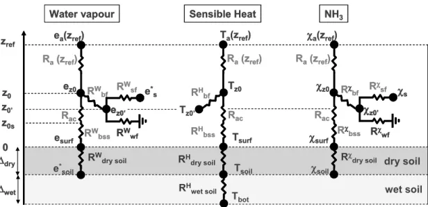
Interactive Discussion the energy balance and the NH3 exchange and so with the same transfer resistances

(aerodynamic, boundary layer, and stomatal) modulus the scalar diffusivities. The NH₃ exchange is directly coupled to the energy balance via the leaf temperature (T_z′

0) and

the surface temperature (Tsurf), and the humidity in the canopy (ez₀), which determine

χ_s,χsurf, and R

χ

wf, respectively. Figure 1 shows the resistance analogue scheme for

5

the heat, water vapour and NH3transfer.

2.1 Aerodynamic, boundary layer, stomatal, soil and “cuticular” resistances

In the following, the exponent or index i refers to either water vapour or NH₃. The diffusivity of NH3 in air,DNH₃, and the diffusivity for water vapour in air,Dw, are taken

asDNH₃=2.29 m 2

s−1andD_w=2.49 m2s−1(Massman, 1998).

10

Aerodynamic resistances.The usual hypothesis is made of similarity between turbulent transfers of scalars, hence the aerodynamic resistances Ra and Rac are supposed

identical for water vapour, heat and NH3(details given in Appendix B).

Boundary layer resistances. Following Shuttelworth and Wallace (1985) and Choud-hury and Monteith (1988), the canopy boundary layer resistances (R_bfi , wherei stands

15

for scalari), are expressed as a function of the leaf boundary layer resistance and wind speed inside the canopy:

R_bfi =

_D

i

D_W

−2/3

· αu

2.a.LAI_ss ·

LW

u(hc)

1/2

·

1−exp

−αu

2 −1

(1)

where LAI_ss is the leaf area index (single sided projected foliage surface), a is a co-efficient equal to 0.01 s m−1/2 (Choudhury and Montheith, 1988), αu is defined by

20

(6)

BGD

6, 71–114, 2009

E. Personne et al.

Title Page

Tables Figures

◭ ◮

Back Close

Full Screen / Esc

Interactive Discussion resistance (Rlitter) for transfer due to the litter laying the soil surface:

R_bssi = 2

κ·u∗_ground ·

_Sc

i

Pr 2/3

+Rlitter (2)

whereSc_i is the Schmidt number for the scalar i (Sc_i=ν_a/D_i,D_i being the diffusivity of the scalar i and ν_a the cinematic viscosity of air), Pr is the Prandtl number, and

u∗_ground is the friction velocity near the soil surface, which is calculated following Loubet

5

et al. (2006):

u∗_ground =

(u∗)2·exp

1.2×LAI_ss×

_z

0s

hc

−1

1/2

(3)

wherez0s is the ground surface roughness length, Rlitter is an additional resistance,

which is fixed at either 2000 s m−1 in order to simulate the transfer through the litter (from soil surface to the top of the litter) or 5000 s m−1in order to take into account the

10

closed stomata of the dead leaves over the soil (Jones, 1992).

Resistance parameterisation forNH3.For the component of transfer where turbulence

is small by comparison with the diffusive processes (Fig. 1), NH3molecular diffusivity

DNH₃ must be considered. Based on Eqs. (1) and (2), the diffusivity ratioℜNH₃ is used

to define the NH3boundary resistances for soil and vegetation (R NH₃

bss andR

NH₃

bf ). ℜNH₃ 15

varies with temperature (Massman, 1998) and is given as:

ℜNH₃ =

DNH₃

D_w =0.92 at 25

◦_C ₍₄₎

Hence, the model takes into account these effects in the boundary layers resis-tances:

  

 

RNH3

bf =

ℜNH₃

−2/3

·R_bf RNH3

=ℜNH

−2/3

·Rbss

(5)

(7)

BGD

6, 71–114, 2009

E. Personne et al.

Title Page

Tables Figures

◭ ◮

Back Close

Full Screen / Esc

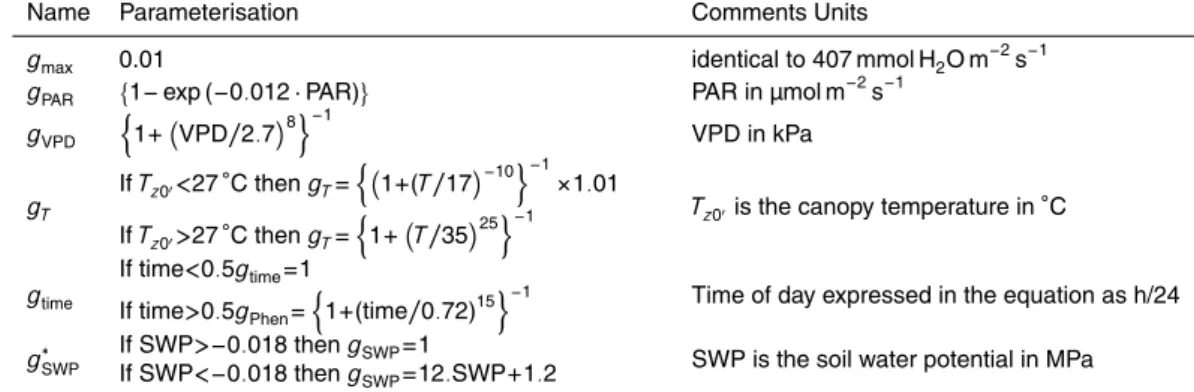
Interactive Discussion Stomatal resistance. The stomatal resistance for a gas compoundi (R_si) is calculated

following Jarvis (1976), as a function of the photosynthetycally active radiation (PAR), and stress functions, with the parameterisation of Pleijel et al. (2004) (Appendix C). Soil resistances. Following Choudhury and Monteith (1988), the dry and wet soil layer resistances for heat conduction are calculated as:

5

R_{dry soil}H =ρa·cp·

∆dry

κdry

(6)

R_{wet soil}H =ρa·cp·

∆wet

κwet

(7)

whereκ is the thermal conductivity, cpspecific heat capacity of air,ρa the air density

and the thickness of each layer. The subscripts wet and dry stands for the wet and the dry layer, respectively.

10

For the gas transfer in the soil, the soil resistance is evaluated according to the dry soil thickness∆dry with the following resistance:

R_{dry soil}i = τsoil·∆dry

p·Di

(8)

wherepis the porosity of the soil,τsoilis a tortuosity factor.

Cuticular resistance.For a simplified approach, cuticular exchanges for water are

sup-15

posed to be negligible compared with stomatal exchange, while for NH3, the resistance

is parameterised without taking into account the chemical reactions with the surface. Hence in SURFATM-NH3, the surface concentration χwf is assumed to be zero with

the resistance depending on microclimate. Following Sutton et al. (1993) and Sutton et al. (1995), cuticular resistance is set toRNH3

wf vary according to air relative humidity

20

(8)

BGD

6, 71–114, 2009

E. Personne et al.

Title Page

Tables Figures

◭ ◮

Back Close

Full Screen / Esc

Interactive Discussion (Sutton et al., 2001; Milford et al., 2001a):

RNH3

wf =R

NH₃

wf min·exp

100−RH 7

(9)

where RH is the relative humidity, andRNH3

wf min=30 s m

−1

.

2.2 Sub-stomatal cavity and soil surface/litter NH3concentration

Following Schjoerring et al. (1998), the compensation point is modelled as resulting

5

from the thermodynamic equilibrium between NH3 in the liquid and in the gas phase

as well as the acid-base equilibrium between NH+₄ and NH₃in the liquid phase:

χ_i=K_HA·K_AC·exp ∆H

0

HA+ ∆H

0

AC

R ·

1 298.15 −

1

T_iK

!!

·Γi (10)

where K_HAand K_ACare equilibrium constants at 25◦C, and∆H0are free enthalpies,R

is the perfect gas constant,TK is the temperature in Kelvin, andΓ is the emission

po-10

tential. SubscriptsHAandAC stand for “Henry” and “dissociation”, respectively; while subscripti designs the compartment considered : the sub-stomatal cavity (s), the in-terface between wet and dry soil (soil), or the ground surface/litter (surf). The temper-atures have the corresponding subscript, except for the sub-stomatal cavity where the temperatureT_s=T_z0′. The compensation point (χi) varies according to the temperature

15

Ti and Γi, where Γi is the non-dimensional ratio [NH+4]/[H+], where brackets denote

concentrations in mol mol−1 of available compound (not bound to soil colloids or leaf cells). Concerning the emission potential for the stomatal pathway, Γs can in some

instances be estimated from measurements of [NH+₄] and the pH of the plant apoplast, or it can represent an adjustment parameter in fitting the model to measured fluxes. In

20

the literature, estimates of Γs are typically in the range 60–5800 (e.g., Loubet et al.,

(9)

BGD

6, 71–114, 2009

E. Personne et al.

Title Page

Tables Figures

◭ ◮

Back Close

Full Screen / Esc

Interactive Discussion plant metabolism (Riedo et al., 2002). In the model scheme used here (Fig. 1),

con-cerning the soil pathway,Γsurf can either be the emission potential of the soil surface

or that of the litter or dead leaves lying on the groundΓlitter, whileΓsoilis the emission

potential at the dry-wet interface in the soil. Various models have examined the con-tributions of fertilisation, the soil water status, the microbiological activity and this “soil

5

compensation point” (Genermont et al., 1998; Pinder et al., 2004). In the following,Γi

will be computed from measured [NH+₄] and [H+].

2.3 Soil water balance

The evolution of the soil water balance is based on a two-layer approach where the soil evaporation leads to a drying of the upper dry layer, and to an increase of the thickness

10

of this dry layer (∆dry) according to Choudhury and Montheith (1988). The plants are

supposed to take up the water in the wet soil only. Hence the transpiration decreases the soil water content of the wet soil and hence the water availability for plants.

2.4 Operational of the model

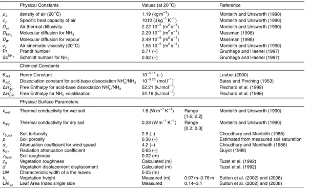
SURFATM-NH3 requires input data of concentration at the reference height, meteo-15

rology, soil and vegetation stand structure. Meteorological forcing includes values of air temperature (T_a), relative humidity (RH), net radiation (Rn) and, wind speed (u) at a reference heightzref and precipitation (Rain). Soil water content is described by the

field capacity (θcc), wilting point (θwp) and dry soil humidity (θHA) in order to define the

soil water availability for plants. The single sided leaf area index (LAI_ss) and the height

20

(10)

BGD

6, 71–114, 2009

E. Personne et al.

Title Page

Tables Figures

◭ ◮

Back Close

Full Screen / Esc

Interactive Discussion 3 Material and methods

3.1 Experimental data

The energy balance model was validated against measurements performed over a grassland field. And the modelled NH3 exchange is compared to NH3 flux and

concentration measurement performed at the same time. The dataset used is briefly

5

described in this section.

The European project GRAMINAE (Grassland Ammonia Interactions Across Eu-rope – Sutton et al., 2002, 2008) was instigated to quantify exchange of NH3 with

grasslands across an East-West transect across Europe. As part of this effort, an integrated experimental campaign took place 18 May–15 June 2000 at a 6.4 ha

ex-10

perimental agricultural grassland of the German Federal Agricultural Research Centre Braunschweig, V ¨olkenrode (52◦18′N, 10◦26′E; 79 m a.s.l.).

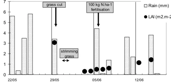
Agronomic conditions in the experiment are described by Sutton et al. (2008) and show a large range of situations to evaluate the model: a) the vegetation was at first tall and dense; b) it was cut on 29 May 2000, and then left for 7 days; and c) the

15

field was fertilized on 6 June with 108 kg N ha−1 as calcium ammonium nitrate. The calendar events are summarized in Fig. 2. During the measurement period before the cut, the canopy heighthc increased from 0.65 to 0.75 m with a single sided leaf area

index (LAIss) of 3.1 m2m−2. After the cut, hc and LAIss were 0.07 m and 0.3 m2m−2

and developed up to 0.32 m and 1.4 m2m−2by 15 June.

20

The model is performed with quarter-hourly time-step in order to take into account the fast changes of surface temperature and energy fluxes and the hypothesis of the stationarity of the climatic data on this time-step (Lumley and Panofsky, 1964). Climatic data of the experimental site (Nemitz et al., 2008), provided inputs forTa, RH, Rn, u

and Rain, with the other input parameters used for the simulations summarized in

25

(11)

BGD

6, 71–114, 2009

E. Personne et al.

Title Page

Tables Figures

◭ ◮

Back Close

Full Screen / Esc

Interactive Discussion temperatures were estimated from measured temperature in the canopy litter and soil

with fine thermocouples.

3.2 Evaluation of heat balance model

As discussed in Nemitz et al. (2008), the measured heat fluxes lead to a lack of clo-sure of the energy balance (R_n=H+λE+G+l ack), by about 30%. However, since the

5

model is based on the energy closure, the heat fluxesH andλE were adjusted so that

H+λE=R_n−G. Based on the arguments of Twine et al. (2000), the bowen ratio was maintained and both H and λE were increased by 29% (Nemitz et al., 2008). The canopy height hc, and the leaf are index were prescribed from measurements. The

measured and modelledH,λE,G,T_z0′ andT_surf are compared against each other for

10

estimating the validity of the heat model.

3.3 Parameterisation of the NH3emission potentialsΓs,ΓsoilandΓlitter

The model inputs for Γs and Γsoil were derived from plant and soil measurements

made during the experiment, which also provided estimates for plant litter (Γlitter). The

measurements of apoplastic, litter and soil [NH+₄] and pH are described by Mattsson

15

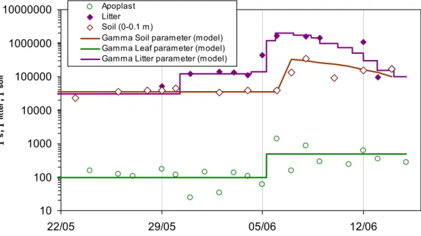
et al. (2008a), Herrmann et al. (2008), and Sutton et al. (2008), with the synthesis of the different values reported by Sutton et al. (2008). Based on this synthesis, we interpolated the measured values to provide simplified profiles of Γs, Γsoil and Γlitter

through the experiment (Fig. 3). The huge range of measured values betweenΓs,Γsoil

andΓlitteris apparent in Fig. 3. Γs values were rather modest, between 100–600, with

20

an increase occurring after fertilization. Values ofΓsoil were much larger, especially

after fertilization, indicating the ground surface as the dominant emission pathway for this period. It is notable, however, thatΓlittervalues were very high in comparison with

the values of Γs and Γsoil, both before and after the cut, while after fertilization Γlitter

increased further, possibly due to the presence of fertilizer ammonium adsorbing to the

25

(12)

BGD

6, 71–114, 2009

E. Personne et al.

Title Page

Tables Figures

◭ ◮

Back Close

Full Screen / Esc

Interactive Discussion The interpolated lines in Fig. 1 provided the input Γ values for the model

simula-tions, using two different approaches, named scenario S1 and scenario S2. In the first approach (S1), the ground surface emission was parameterised using the measured values ofΓsoil, with hypothesis that the NH3 comes from the boundary between wet

and dry soil (level soil in Fig. 3). Therefore, the value ofΓsoil was associated with the 5

temperature at this level (T_soil∗ ) and the soil resistance (Rsoil). In the second approach

(S2), the ground surface emission was parameterised using the measured values of Γlitter, with the hypothesis that the associated temperature is that of the soil surface

(T_ss- level surf in Fig. 1), with the stomata of the litter assumed to be inactive providing an additional resistanceRlitter=5000 s m−

1

in the simulation.

10

In both approaches, the modelledΓsis used to estimate the sub-stomatal cavity NH3

concentrationχ_s using based on Eq. (8).

4 Results

The simulations of SURFATM-NH₃ were compared with the detailed energy bal-ance measurements reported by Nemitz et al. (2008) and with the measured mean

15

NH3 fluxes determined by aerodynamic gradient method, as reported by Milford et

al. (2008), including appropriate corrections for advection where necessary (Loubet et al., 2008). For certain days there was significant uncertainty in the mean fluxes, so that Milford et al. (2008) also reported an “alternative estimate” of the flux. Further compari-son with flux measurements using a surface dispersion model (Loubet et al., 2007) and

20

(13)

BGD

6, 71–114, 2009

E. Personne et al.

Title Page

Tables Figures

◭ ◮

Back Close

Full Screen / Esc

Interactive Discussion 4.1 Energy budget

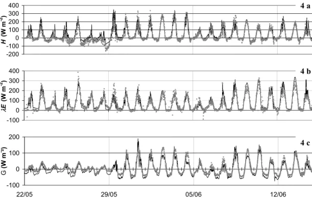
No calibrations were used for the part of the model which treats the energy budget. Figure 4 represents the various fluxes of the energy budget. The corrections of Twine et al. (2000), accounting for fluctuation methods and direct measurements of Rn, were applied and allow a coherent energy budget to be estimated with independent

mea-5

surements ofH and λE: the model shows a close agreement to the measured fluxes throughout the comparison (Table 2). A major change in fluxes magnitude occurs from the 29 May. The grassland cut led increased the total heat flux (H) and the soil heat conduction (G). This clear change is not observed for the modelled latent heat flux (λE) on 29 May, and may result from a transient increase in evaporation and drying of

10

the grass cuttings prior to their removal.

4.2 Temperature

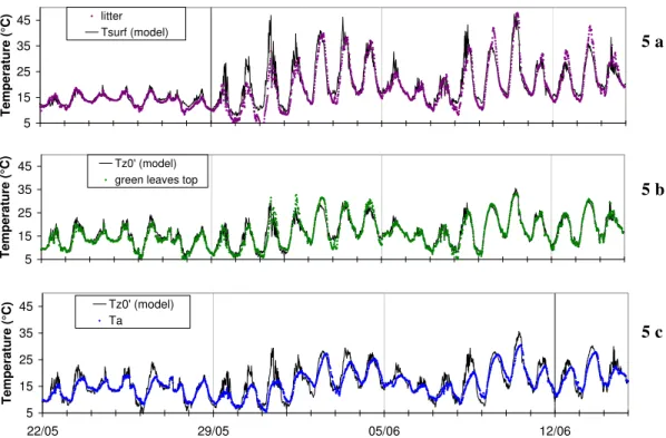
The modelled surface temperature of the soil and the foliage are the equilibrium vari-ables of the energy budget. These varivari-ables are the key-connections between the energy budget and the ammonia exchange. Figure 5 shows the results of measured

15

and modelled temperatures before and after the cut. The modelled soil surface and leaf temperature (TsurfandTz0′) are higher than the air temperature (Ta) during the day, and

vice versa during the night: the cooling and warming process of the canopy surfaces seems to be in good agreement with the measurements. During the day, the vegeta-tion temperature is ranged between the measurements of the top and the bottom of

20

the canopy. The agreement between the model and the measurements is within 2.5◦C forT_z0′ and so the foliage temperature and 4◦C forT_surf, the soil surface temperature. The worst agreement is just following the cut where the difference between measured and modelled temperatures reaches 4◦C for Tz0′ and 10◦C for T_surf. However before the cut, the agreement is much better 1◦C forT_z0′and 2◦C forT_surf. It can be underline

25

(14)

BGD

6, 71–114, 2009

E. Personne et al.

Title Page

Tables Figures

◭ ◮

Back Close

Full Screen / Esc

Interactive Discussion for the difference (T_a−Tlitter)

4.3 Ammonia fluxes and dynamics of the emission potential

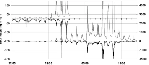
Figure 6 presents the comparison between modelled total NH3 fluxes and the

mea-sured NH3 fluxes above the field. From 21 to 29 May (before the cut), the

NH₃ exchanges ranged between a deposition of −50 ng NH₃m−2s−1 to an

emis-5

sion of +40 ng NH3m− 2

s−1. Following cutting, NH3 emissions increased up to up

500 ng NH3m− 2

s−1(Fig. 6). These emissions are an order of magnitude greater than the typical emission observed over the grassland previous to cutting. Following fertil-ization on 6 June, the fluxes immediately increased up to 2000 ng NH3m−

2

s−1. These high emission values continued few days before progressively decreasing to similar

10

emission fluxes prior to fertilization at daytime maxima near 500 ng NH₃m−2s−1. The typical diurnal pattern of emission fluxes after the cut and the fertilisation typically ex-hibited a clear increase in emission starting at 06:00 UT and reverting to near zero at 20:00 UT (Fig. 6).

The simulations are based on two scenarios: the soil emission scenario (S1) and

15

the litter emission scenario (S2). Both the simulations using litter and soil emissions reproduce the diurnal dynamics of emissions. Prior to the cut, the temporal dynamics of both models are similar, with the litter model most close to the absolute value of the measurements. The two scenarios reproduce satisfactorily the fluxes before the cut (with a tendency for the model to give more emissions periods than the measurements)

20

as well as a week after fertilisation (with higher modelled emissions at nights). The two scenario however fail to reproduce the pulse of emission the day of the cut (29 May). Moreover, the two scenarios show deposition the 28 May between 06:00 UT and 12:00 UT, while the measurements show small emissions, possibly denoting a local advection episode (Loubet et al., 2006).

25

(15)

BGD

6, 71–114, 2009

E. Personne et al.

Title Page

Tables Figures

◭ ◮

Back Close

Full Screen / Esc

Interactive Discussion overestimates it by roughly 30%, except on the 1 June, where it correctly predicted the

fluxes.

SURFATM-NH3clearly simulates the increase in NH3emission following cutting

us-ing both the litter and soil emission parameterisations. It may be noted from Fig. 3 (bioassay Gammas) that the parameterised Γsoil was unchanged following cutting. 5

Therefore, the increased NH3 emissions in the soil source simulation are a result

of other factors, primarily the removal of the overlying canopy (which would recap-ture a fraction of the ground surface emission) and the warmer ground temperarecap-tures (Fig. 5). However, the modelled soil source (S1) does not generally explain all the in-crease in NH3 fluxes observed during this period (apart from 30–31 May). The larger 10

emissions on 1–4 June are more closely simulated using the litter NH₃ source (S2), including the larger values on 3 June.

For the post-fertilization period, both the soil source and litter source parameterisa-tions (S1 and S2) demonstrate the further increase in NH₃ emission, which is closely coupled to the changing measured values ofΓsoil,Γlitterover this period (Fig. 3). It is no-15

table that the simulation using the soil source parameterisation does not reproduce the initial emission after fertilization on 5 June, since measured soil [NH+₄] only increased on 6–7 June, which may reflect sampling uncertainty, linked also with soil sampling depth over the layer 0–10 cm. Conversely, the litter parameterisation (S2) over esti-mates emissions on 8–10 June, while both parameterisations reveal the subsequent

20

decrease in emissions on 11–14 June.

In details during the two days following fertilisation, the soil emission scenario show almost no NH3emissions, while the litter emission scenario reproduces fairly well the

magnitude and the pattern of the fluxes (especially the night time emissions during the nights 5–6 June and 6–7 June). Following the pattern ofΓsoil (Fig. 3), three days 25

after fertilisation, the soil emission scenario start to give larger NH3emissions, but still

smaller than the measured ones, while the litter emission scenario agree very well with measured NH3fluxes. From day 4 to day 6 after fertilisation, the soil emission scenario

(16)

BGD

6, 71–114, 2009

E. Personne et al.

Title Page

Tables Figures

◭ ◮

Back Close

Full Screen / Esc

Interactive Discussion which overestimates the fluxes both during nights and during days.

5 Discussions

The close agreement for H, λE and G fluxes (Fig. 4) between measurements and simulations ensures a consistent calibration for the physical and biological parameters (Table 1). It can be supposed that the values used for the stomatal resistance and

5

soil thermal conductivities are well adapted to the experimental site. The correction of Twine et al. (2000) was used to have a closing measured energy budget. However, without Twine’s corrections the modelled latent heat flux (λE) is overestimated by 26%, while the modelled sensible heat flux (H) is only overestimated by 11%, hence suggest-ing that the measuredλE was probably underestimated, which confirms the analysis

10

of Nemitz et al. (2008).

The litter is taken into account in the resistance scheme of the energy balance model with an additional resistance (Rlitter). This litter layer reduces the transfer of sensible

heat between the soil and the canopy (largerR_drysoilH ) and reducesG, which was over-estimated by the model at night by 28%. The additional “litter” resistance of 2000 s m−1

15

almost decreases the difference between modelled and measuredG at night. The lit-ter would also induce an additional walit-ter “reservoir” in the canopy which would lead to evaporation during the day and condensation at night, hence modifying the energy partition at the ground (Tuzet et al., 1993).

The modelled canopy temperatureTz0′is close to the measured top green leaves, by

20

less than 2◦C, which is smaller than the difference between the measuredTa andTz0′ (Fig. 5). The soil surface temperatureTsurf is also well modelled except for three days

following the cut, where it reaches 3 to 6◦C above the measuredTsurf. This

overestima-tion is certainly linked with the presence of the grass left on the field (striming in Fig. 2), which would have increase the resistance for heat transfer at the ground surface.

(17)

BGD

6, 71–114, 2009

E. Personne et al.

Title Page

Tables Figures

◭ ◮

Back Close

Full Screen / Esc

Interactive Discussion 5.1 Uncertainty in stomatal resistance and emission potential

The good agreement between the modelled and measured heat fluxes and tempera-tures also implies that the stomatal resistanceRsW,R

NH₃

s and the canopy temperatures

(T_z0′ and T_surf, respectively), and humidity are all correctly predicted. This is without questioning the Twine et al. (2000) correction which drastically changes R_s. A new

5

parameterisation should multiplicateRsW by two in order to reproduce the range of the

latent heat flux directly measured, without correction.

An increase of 100% of the stomatal resistance increases the heat exchanges and increases the gap between model and measurements by 18% for the heat fluxesH

and 2% for the soil heat conductionG while this variation for the stomatal resistance

10

induces a decrease of 25% for the latent heat fluxλE. Such variation of the stomatal resistance induces only a small change of the temperature smaller than 0.5◦C. The uncertainty on R_s based on the error of H, λE and G induces a small effect on the surface temperatures

The temperaturesTz0′ andT_surf are very sensitive parameters of the NH₃ exchange

15

model since the compensation pointsχ_s andχsurfare exponentially dependent to

tem-perature (Eq. 8). The coupling between the energy balance model and the pollutant exchange model is essentially made viaTz0′ and T_surf. Hence the fact that these two modelled temperatures are in agreement with the measured ones within 2◦C (in gen-eral), implies a potential error onχ_sandχsurfof 20%.

20

5.2 Dynamic of the exchanges

Examining the period prior to the cut (Fig. 6a), NH₃fluxes are lower than 100 ng m−2s−1 and deposition was predominant. This deposition would have been governed by the plant exchanges according to the covering foliage of plant (LAI_ss=3). Similar fluxes have been reported elsewhere for managed grassland (Milford et al., 2001a) and as in

25

our experiment, deposition fluxes are close to 50 ng NH3m− 2

(18)

BGD

6, 71–114, 2009

E. Personne et al.

Title Page

Tables Figures

◭ ◮

Back Close

Full Screen / Esc

Interactive Discussion of the cuticular deposition. For ammonia, air water content (expressed as relative

humidity or vapour pressure) is a determinant variable, and in this simplified approach based on the parameterisation of Milford et al. (2001b), only this variable is sufficient to reproduce much of the pattern in deposition. In fact, this approach is simple and operational with only climatic forcing (RH at the reference height zref), but does not 5

reproduce NH3 desorption processes (Sutton et al., 1998a; Flechard et al., 1999) or

specific microclimate in the vicinity of the foliage. However it remains consistent for the model because this approach is validated for various conditions and plant surface types (van Hove et al., 1989; Sutton et al., 1995; Nemitz et al., 2001). The first improvement could be simply done by using the relative humidity of the air in the vicinity of the foliage

10

(at the levelz0′) instead of the air ambient RH on condition that the parameterisation of Milford et al. (2001a) remains adapted to this change of compartment level (z′₀instead ofzref). The cuticular exchanges could also be treated in a dynamical approach, as

an electric capacitor with a surface chargeχwf, which may be released under certain

conditions (Sutton et al., 1998b). The exchange conditions are related to the surface

15

chemical processes, the air vapour pressure and the temperatures, and to the climatic events (rainfall and surface leaching) (Flechard et al., 1999). The potential importance of these cuticular adsorption/desorption processes for the Braunschweig dataset are investigated by Burkhardt et al. (2008).

After the vegetation is cut, the role of the ground surface exchange enhances, as

20

does the influence of the ground surface temperature. The role of ground temperature was particularly important during the period after cutting where soil surface tempera-ture increased by 15◦C during the day in comparison with values at night.

The ammonia exchanges from plant were parameterised by values of emission po-tential ranged between 100–600 (Fig. 3), which are typical of other similar

measure-25

ments (e.g., Loubet et al., 2002). For the soil emission following N fertilisation, the simple linear decrease from a maximum value ofΓsoil=300 000 to a value of 40 000 ten

(19)

BGD

6, 71–114, 2009

E. Personne et al.

Title Page

Tables Figures

◭ ◮

Back Close

Full Screen / Esc

Interactive Discussion emission potential should be take into account the degradation on the soil surface and

the dilution or leaching with water soil in order to have an improvement of the simulated results in comparison with measurements, and these aspects should be considered in future work. This result demonstrates the influence of the agronomic/soil management and the link between the microclimate and the pollutant exchange. Similarly, while

5

overall agreement was found between the model and the measurements, as well as the results of parallel cuvette measurements (David et al., 2008), the measuredΓsoil

andΓlittervalues must also be considered as uncertain. For example, mineralization of

NH+₄ in litter may be considered will depend on moisture availability, so that loss of NH3

to the atmosphere will deplete Γlitter values substantially until more mineralization is 10

able to occur. Such dynamics, not included in the present simulation can easily explain the differences between model and measurements that were observed.

5.3 Partition of NH₃fluxes between the soil, the litter and the stomata

Baring in mind thatΓs,ΓsoilandΓlitterwere prescribed, the model with the litter scenario

agrees very well with the measurements over a period which shows a change two order

15

of magnitude of the NH3flux (Fig. 6). The only hypothesis made were that the litter had

an additional resistanceRlitter=5000 s m− 1

of the order of closed stomata (Jones, 1992; Weyers and Meidner, 1990), and that the bulk solution of the leaves was in equilibrium with the atmosphere, which implies that the NH+₄ measured in the bulk extracts is freely available, and that the bulk pH is representative of that solution. The good agreement

20

between the model and the measurements allows to investigate the origin of the flux with the model:

Before the cut. The good agreement at the transition from uncut to cut grassland, with a constantΓlitter/Γsoil(Fig. 3), and the fact that both scenario agree quite well before the

cut shows that before the cut, the stomata are absorbing most of the NH₃emitted from

25

the ground. The model shows that between 5 and 20 ng NH3m

−2

(20)

BGD

6, 71–114, 2009

E. Personne et al.

Title Page

Tables Figures

◭ ◮

Back Close

Full Screen / Esc

Interactive Discussion of−5 ng NH3m−

2

s−1due to vegetation absorption (Fig. 7). However, the ground NH3

emissions still have a great impact on the overall NH3exchange by increasing the NH3

concentration around the leaves. Based on the model, if there was no source at the ground before the cut, the NH3 flux within the canopy would be a deposition flux of 5

to 40 ng NH₃m−2s−1. The fact that the soil scenario (S1) shows a slight offset in the

5

predicted flux before the cut probably indicates an overestimation of the litter resistance during that period.

After the cut. The NH3fluxes increase following the cut (Fig. 6). There is some

discus-sion in the recent literature about whether the cut would increase the stomatal com-pensation point as a result of remobilisation (David et al., 2008). However, Loubet et

10

al. (2002) have found no increase inΓs immediately following the cut but a slight

in-crease later. Moreover the levels ofΓs in Loubet et al. (2002) were comparable to the

Γs found in this study and they can not explain the levels of emissions found after the

cut. The fact that the measured NH3fluxes lie between the litter emission scenario and

the soil emission scenario strongly suggests that the source of NH3emission following 15

the cut is the ground. The increased NH₃emissions following the cut can be explained by two factors: (i) the weight of the stomatal sink is reduced by the cut, and (ii) the temperature of the litter/soil changes from a daily mean of 15±10◦C before the cut to a daily mean of 20±15◦C after the cut (Fig. 5). Baring in mind that a 5◦C increase of the surface emitting NH3induces a twofold increase in emissions (Eq. 10), this means 20

that following the cut, the maximum emission from the litter is multiplied by 8, which is what is observed in Fig. 7. The fact that the litter emission scenario (S2) agrees better with the measurements than the soil emission scenario (S1) can be explained by the soil temperature being roughly 2–3◦C smaller than the litter temperature. This is clear on the 31 May, where the soil temperature is 5◦C smaller than the litter

temper-25

ature and the soil emission scenario gives NH₃ emissions twice as small as the litter emission scenario.

However, the litter emission scenario tends to overestimates the NH3 fluxes

(21)

BGD

6, 71–114, 2009

E. Personne et al.

Title Page

Tables Figures

◭ ◮

Back Close

Full Screen / Esc

Interactive Discussion at the litter being not a perfect equilibrium as expressed in Eq. (8), (ii) the Γlitter

be-ing overestimated by the extraction technique, (iii) the soil surface temperature bebe-ing overestimated by the model during that period, (iv) an underestimation of the litter re-sistance, (v) the progressive transfer of the ammonium from the litter to the soil, or (vi) the cuticular exchange which could be higher than modelled in this study. Although all

5

these hypotheses are plausible, they can not be proven with the available data.

After the fertilisation. The fertilisation induces an increases of the NH3 fluxes which

is well reproduced by the model (Fig. 6) due to the Γlitter increasing just following the

application of fertiliser (and two days later Γsoil increases also). The NH3 emissions

during the night between the 5 and the 6 June and the 6 and the 7 June is typical of

10

non-stomatal emissions and is well reproduces by the litter emission scenario. The soil emission scenario gives deposition NH₃fluxes the 5 and 6 June, which shows that

χz0<χa(zref) (Fig. 1), hence demonstrating that the soil emission scenario (Γsoil, and

Rlitter) fails to reproduce the emissions with the observed increase of NH3

concentra-tion. However, the soil emission scenario gives progressively increasing NH₃

emis-15

sions and matches the measured emissions six days following the fertilisation, while in the same period, the litter emission scenario gives too large emissions. Hence the simulations shown in Fig. 6 suggest that the main source following fertilisation is the litter which has effectively received the ammonium-nitrate pellets, and which contain the water (due to condensation) necessary for dissolving these pellets. However, the

20

overestimation of the litter scenario in the following days (8 to 10 June) is still unclear. It might be due to (i) the litter temperature being overestimated by the model (Fig. 5) (ii) the litter resistanceRlitterchanging due to either a migration of NH+4 to the bottom of

the litter, or (iii) NH+₄ being not freely available due to metabolic changes.

6 Conclusions

25

(22)

BGD

6, 71–114, 2009

E. Personne et al.

Title Page

Tables Figures

◭ ◮

Back Close

Full Screen / Esc

Interactive Discussion based on the prescription of measured canopy height and leaf area index. The model

also succeeds in simulating the leaf and ground surfaces temperatures.

The overall agreement between the energy balance model and the measurements implies that the stomatal resistance is correctly modelled. The correct predictions of temperatures and stomatal resistance validates the coupling between the energy

bal-5

ance model and the NH3 exchange model, since NH3 exchange is mainly influenced

by the stomatal resistance and the surface concentration which is exponentially linked to the temperature.

Using measured emission potentials of the appoplasm and the litter, the NH3

ex-change model successfully simulates the measured NH3 fluxes during the cut and 10

fertilisation period, over which the fluxes changes by two order of magnitude. The analysis of the partitioning of the fluxes between the model compartments, especially before and after the cut shows that the grassland can be described as the superposi-tion of a litter/soil surface source and a stomatal sink. Of the different compensation points simulated, i.e. for green leaves, litter and the soil surface, the classical role of

15

a foliar compensation point is rather different in the present study. Here, instead of the net flux depending on the balance of the air concentration and the foliar (stomatal) compensation point, the overall canopy compensation point and net fluxes are influ-enced to a large degree by emission potentials from the leaf litter. Prior to the cut, these emissions are mostly recaptured by the overlaying canopy, while they dominate

20

net emissions following cutting and fertilization. Future work should thus pay more at-tention to the dynamics of nitrogen cycling with conditions at the litter and soil surface. The agreement between the modelled and measured NH₃fluxes hence demonstrate (i) the necessity to consider two layers (stomata and litter/soil surface), (ii) the need to couple with an energy balance model which can simulate the leaf and litter/soil surface

25

temperature, and (iii) the interests in using NH₃ emissions potentials in the litter and the apoplasm, which can be measured in the field.

(23)

BGD

6, 71–114, 2009

E. Personne et al.

Title Page

Tables Figures

◭ ◮

Back Close

Full Screen / Esc

Interactive Discussion and leaf area index. This emphasises the need to improve our understanding of the

seasonal pattern of these emissions potential, which implies a better understanding of the ammonium metabolism and pH regulation in the litter as well as the apoplasm of growing leaves, and their interaction with the soil.

Overall, the well behaviour of the coupled SURFATM-NH₃ provides a basis that is

5

also suited for application to other gaseous compounds. This model thus provides a simplified generalised approach for application to atmospheric transport modelling.

Appendix A

Description of the energy balance model

10

Radiation, heat and vapour transfer. The net absorption of radiation by the vegetation and the soil Rn_T is given by (Varlet-Grancher et al., 1989; Tuzet and Perrier, 1992):

Rn_T =Rnveg+Rnsoil (A1)

Rnveg=RnT ·exp(−kRn·LAI) (A2)

The energy received by the leaves is partitioned between latent and sensible heat

15

components, while at the soil surface, an additional conduction heat flux is included:

Rnveg=Hveg+λEveg (A3)

Rnsoil=Hsoil+λEsoil+G (A4)

The total heat fluxH_T , and the total latent heat fluxλE_T are calculated as:

H_T =ρ_a·c_p· Ta−Tz0

R_a (A5)

20

λET =

ρa·cp

γ ·

ea−ez0

(24)

BGD

6, 71–114, 2009

E. Personne et al.

Title Page

Tables Figures

◭ ◮

Back Close

Full Screen / Esc

Interactive Discussion In the canopy, the flux partition is given by:

Hveg=ρa·cp·

T_z0−Tz0′

R_bfH (A7)

λEveg=

ρa·cp

γ ·

ez0−ez0′

R_bfW =

ρa·cp

γ ·

ez0−e

∗

s

R_bfW +R_sfW (A8)

At the soil surface, the heat fluxes are given by:

Hs =ρa·cp·

Tz0−Tsurf

R_bssH +R_ac (A9)

5

λEs =

ρa·cp

γ ·

ez0−esurf

R_bssW +R_ac =

ρa·cp

γ ·

ez0−e

∗

soil

R_bssW +R_ac+R_{dry soil}W (A10)

G=λwet·

Tbot−Tsoil

∆wet

=ρa·cp·

Tbot−Tsoil

R_{wet soil}H (A11)

As in Choudhury and Monteith (1988), the volumetric heat capacity for air in Eq. (A11) appears for algebraic convenience (λwet is the thermal conductivity extending from the

soil bottom to the soil wet-dry boundary, over a thickness∆wet). The resolution of the 10

(25)

BGD

6, 71–114, 2009

E. Personne et al.

Title Page

Tables Figures

◭ ◮

Back Close

Full Screen / Esc

Interactive Discussion Appendix B

Details of the aerodynamic resistances

Aerodynamic resistance above the canopy. The aerodynamic resistance for scalar above the canopy (R_a), at heightzref, is calculated as:

5

Ra=

1

κ2_·_u₍_Z₎ ·

ln

_Z

z0

−ψH(Z/L) ln

_Z

z0

−ψM(Z/L)

(B1)

whereκis the Von-K `arm `an constant (0.4),Z=zref−d,d being the displacement height,

u(Z) is the wind speed, z₀ is the canopy roughness height, L is the Monin-Obukhov length, andΨH andΨM are the stability correction functions for heat and momentum,

respectively. The correction functions of Dyers and Hicks (1970) are used.

10

Aerodynamic resistance inside the canopy. Considering that the foliage has a homo-geneous vertically distribution, the windspeed decreases exponentially (Cowan, 1965):

u(z)=u(hc)·exp

αu·

z h_c −1

(B2)

withu(z), the wind speed inside the canopy at height z,u(hc) the wind speed at the

canopy height (h_c),α_uis the attenuation coefficient for the decrease of the wind speed

15

inside the cover (Raupach et al., 1996). With the hypothesis that the decrease of the diffusivity is proportional to the decrease of the wind speed inside the canopy, the aerodynamic resistance inside the cover (R_ac) takes the form:

R_ac= hc·exp(αu)

α_w·K_M(h_c) ·

exp (−α_u·z0s·hc)−exp

₋_α

u(d+z0)

h_c

(B3)

where KM(hc) is the eddy diffusivity coefficient at canopy height hc, and z0s is the

20

ground surface roughness length.

(26)

BGD

6, 71–114, 2009

E. Personne et al.

Title Page

Tables Figures

◭ ◮

Back Close

Full Screen / Esc

Interactive Discussion Appendix C

Details of the stomatal resistance model.

Following Pleijel and al (2004), the stomatal conductance for the gasi gis per leaf are

is calculated as:

5

gi_s= Di

D_w max{gmin;gmax(gVPD·gT ·gPAR·gSWP·gtime)} (C1)

whereDi andDw are the molecular diffusivities of the gasi and of water vapour in air,

respectively;gmin andgmaxdenote, respectively, the minimum and maximum stomatal

conductance allowed for a certain species by the model. The factorsgVPD, gT,gPAR

andgtimerepresent the short-term effects of leaf-to-air vapour pressure difference, leaf 10

temperature, photosynthetically active radiation and time of day. The influence of time-of-day is an effect of the internal water potential of the plant (Livingston and Black, 1987). The effect of soil water potential is reflected by the gSWP factor. Although at

very high concentrations NH3can have an effect on stomata aperture (van Hove et al.,

1989), at normal ambient concentrations this effect is expected to be minimal. So, no

15

effect of ammonia on gi_s is included in the present implementation of the model. As the fluxes from foliage surface integrate the exchanges from the individual leaves, the canopy stomatal resistance for water is estimated as:

R_sW =(g_s)−1=





LAI

Z

0

gw_s

·dLAI′ 

 −1

(C2)

Acknowledgements. The authors gratefully acknowledge funding of this work by under the Eu-20

(27)

BGD

6, 71–114, 2009

E. Personne et al.

Title Page

Tables Figures

◭ ◮

Back Close

Full Screen / Esc

Interactive Discussion References

Anderson, N., Strader, R., and Davidson, C.: Airborne reduced nitrogen: ammonia emissions from agriculture and other sources, Environ. Int., 29, 277–286, 2003.

Bates, R. G. and Pinching, G. D.: Dissociation constant of aqueous ammonia at 0 to 50◦C from m.f studies of the ammonium salt of a weak acid, Am. Chem. Soc. J., 72, 1393–1396, 1950. 5

Bobbink, R.: Effect of nutrient enrichment in Dutch chalk grassland, J. Appl. Ecol., 28, 28–41, 1991.

Bouwman, A. F., Lee, D. S., Asman, W. A. H., Dentener, F. J., and van der Hoek, K. W.: A global high-resolution emission inventory for ammonia, Global Biogeochem. Cy., 11, 561– 587, 1997.

10

Burkhardt, J., Flechard, C. R., Gresens, F., Mattsson, M., Jongejan, P. A. C., Erisman, J. W., Weidinger, T., Meszaros, R., Nemitz, E., and Sutton, M. A.: Modeling the dynamic chemical interactions of atmospheric ammonia and other trace gases with measured leaf surface wet-ness in a managed grassland canopy, Biogeosciences Discuss., 5, 2505–2539, 2008, http://www.biogeosciences-discuss.net/5/2505/2008/.

15

Carsel, R. F. and Parrish, R. S.: Developping joint probablility distributions of soil water retention characteristics, Water Resour. Res., 24, 755–769, 1988.

Choudhury, B. J. and Monteith, J. L.: A four-layer model for the heat budget of homogeneous land surfaces, Q. J. Roy. Meteor. Soc., 114, 373–398, 1988.

Cowan, I. R.: Transport of water in soil plant atmosphere system, J. Appl. Ecol., 2, 221–239, 20

1965.

David, M., Loubet., B., Cellier, P., Mattsson, M., Schjoerring, J. K., Nemitz, E., Roche, R., Riedo, M., and Sutton M. A.: Ammonia sources and sinks in an intensively managed grassland using dynamic chambers, Biogeosciences Discuss., submitted, 2008.

David, M., Roche, R., Mattsson, M., Sutton, M. A., D ¨ammgen, U., Schjoerring, J. K., and 25

Cellier, P.: The effects of management on ammonia fluxes over a grassland using dynamic chambers, Biogeosciences Discuss., submitted, 2008.

Dragosits, U., Theobald, M. R., Place, C. J., Lord, E., Webb, J., Hill, J., ApSimon, H. M., and Sutton, M. A.: Ammonia, emission, deposition and impact assessments at the field scale: a case of study of sub-grid spatial variability, Environ. Pollut., 117, 147–158, 2002.

30

(28)

BGD

6, 71–114, 2009

E. Personne et al.

Title Page

Tables Figures

◭ ◮

Back Close

Full Screen / Esc

Interactive Discussion

Erisman, J. W., and Wyers, G. P.: Continuous measurements of surface exchange of SO₂and NH₃ : implications for their possible interaction in the deposition process, Atmos. Environ., 27, 1937–1949, 1993.

Fangmeier, A., Hadwiger-Fangmeier, A., Van der Eerden, L., and J ¨ager, H. J.: Effects of atmo-spheric ammonia on vegetation – a review, Environ. Pollut., 86, 43–82, 1994.

5

Farquhar, G. D., Firth, P. M., Wetselaar, R., and Wier, B.: On the gaseous exchange of ammonia between leaves and the environment: determination of the ammonia compensation point, Plant Physiol., 66, 710–714, 1980.

Flechard, C., Fowler, D., Sutton, M. A., and Cape J. N.: Modelling of ammonia and sulphur dioxide exchange over moorland vegetation, Q. J. Roy. Meteor. Soc., 125, 2611–2641, 1999. 10

Fowler, D., Cape, J. N., and Unsworth, M. H.: Deposition of atmospheric pollutants on forest, Phil. Trans. Roy. Soc. London B., 324, 247–265, 1989.

Freibauer, A.: Regionalised inventory of biogenic greenhouse gas emissions from European agriculture, Eur. J. Agron., 19, 153–160, 2003.

Ganzeveld, L. N., Lelieveld, J., Dentener, F. J., Krol, M. C., and Roelofs, G.-J.: Atmosphere-15

biosphere trace gas exchanges simulated with a single-column model, J. Geophys. Res., 107(D16), 4297, doi:10.1029/2001JD000684, 2002.

Genermont, S., Cellier, P., Flura, D., Morvan, T., and Laville, P.: Measuring ammonia fluxes after slurry spreading under actual field conditions, Atmos. Environ., 32, 279–284, 1998. Gr ¨unhage, L. and Haenel, H.-D.: PLATIN (PLant-ATmosphere-Interaction) I : A model of plant-20

atmosphere interaction for estimating absorbed doses of gaseous air pollutants, Environ. Pollut., 98, 37–50, 1997.

Guyot G.: Physics of the Environment and Climate. John Wiley, Chichester, 632 pp., 1998. Hensen, A., Nemitz, E., Flynn, M., Blatter, A., Jones, S., K., Sørensen, L. L., Hensen, B.,

Pryor, S., Jensen, B., Otjes, R. P., Cobussen, J., Loubet, B., Erisman, J. W., Gallagher, M. 25

W., Neftel, A., and Sutton, M. A.: Inter-comparison of ammonia fluxes obtained using the Relaxed Eddy Accumulation technique, Biogeosciences Discuss., submitted, 2008.

Herrmann, B., Mattsson, M., Jones, S. K., Cellier, P., Milford, C., Sutton, M. A., Schjoerring, J. K., and Neftel, A.: Vertical structure and diurnal variability of ammonia exchange potential within an intensively managed grass canopy, Biogeosciences Discuss., 5, 2897–2921, 2008, 30

http://www.biogeosciences-discuss.net/5/2897/2008/.

(29)

BGD

6, 71–114, 2009

E. Personne et al.

Title Page

Tables Figures

◭ ◮

Back Close

Full Screen / Esc

Interactive Discussion

Water Air Soil. Poll., 36, 311–330, 1987.

Husted, S. and Schjorerring, J. K.: Apoplastic pH and ammonium concentration in leaves of Brassica napus L., Plant Physiol., 109, 1453–1460, 1995.

Husted. S., Schjorerring, J. K, Nielsen, K. H., Nemitz, E., and Sutton, M. A.: Stomatal compen-sation points for ammonia in oilseed rape plants under field conditions, Agr. Forest. Meteorol., 5

105, 371–383, 2000.

Hyde, B. P., Carton, O. T., O’Toole, P., and Misselbrook, T. H.: A new inventory of ammonia emissions from Irish agriculture, Atmos. Environ., 37, 55–62, 2003.

Jarvis, P. G.: The interpretation of the variation in leaf water potential and stomatal conductance found in canopies in the field, Phil. Trans. Roy. Soc. London. B, 273, 375–391, 1976

10

Jones, H. G.: Plants and Microclimate. A Quantitative Approach to Environnemental Plant Physiology, Cambridge University Press, 428 pp., 1992.

Krupa, S. V.: Effects of ammonia (NH₃) on terrestrial vegetation: a review, Environ. Pollut., 124, 179–221, 2003.

Li, C., Zhuang, Y., Cao, M., Crill, P., Frolking, S., Moore, B., Salas, W., Song, W., and Wang, 15

X.: Comparing a process-based agro-system model to the IPCC methodology for developing a national inventory of N₂O emissions from arable lands in China, Nutr. Cycl. Agrosys., 60, 159–175, 2001.

Livingston, N. J. and Black, T. A.: Stomatal characteristics and transpiration of three species of conifer seedlings planted on a high elevation south-facing clear-cut, Can. J. Forest Res., 17, 20

1273–1282, 1987.

Loubet, B.: Mod élisation du d ép ôt sec d’ammoniac atmosph érique à proximit é des sources, Ph-D. Th ésis, 329 pp., Paul Sabatier University, Toulouse, France, 2000.

Loubet, B., Milford, C., Sutton, M. A., and Cellier, P.: Investigation of the interactions between sources and sinks of atmospheric ammonia in an upland landscape using a simplified dis-25

persion exchange, J. Geophys. Res., 106(D20), 24 183–24 195, 2001.

Loubet, B., Milford, C., Hill, P. W., Tang, Y. S., Cellier, P., and Sutton, M. A.: Seasonal variability of apoplastic NH+₄ and pH in an intensively managed grassland, Plant Soil, 238, 97–110, 2002.

Loubet, B., Cellier, P., Genermont, S., Laville, P., and Flura, D.: Measurement of short-range 30

dispersion and deposition of ammonia over a maize canopy, Agr. Forest Meteorol., 114, 175–196, 2003.