Inversion of CO and NO<sub>x</sub> emissions using the adjoint of the IMAGES model

(1)

ACPD

4, 7985–8068, 2004

Inversion using IMAGES model

J.-F. M ¨uller and T. Stavrakou

Title Page

Abstract Introduction

Conclusions References

Tables Figures

◭ ◮

Back Close

Full Screen / Esc

Print Version

Interactive Discussion

EGU Atmos. Chem. Phys. Discuss., 4, 7985–8068, 2004

www.atmos-chem-phys.org/acpd/4/7985/ SRef-ID: 1680-7375/acpd/2004-4-7985 European Geosciences Union

Atmospheric Chemistry and Physics Discussions

Inversion of CO and NO

_x

emissions using

the adjoint of the IMAGES model

J.-F. M ¨uller and T. Stavrakou

Belgian Institute for Space Aeronomy, Brussels, Belgium

Received: 5 October 2004 – Accepted: 10 November 2004 – Published: 6 December 2004 Correspondence to: J.-F. M ¨uller (jfm@aeronomie.be)

(2)

ACPD

4, 7985–8068, 2004

Title Page

Tables Figures

◭ ◮

Back Close

Full Screen / Esc

Print Version

EGU

Abstract

We use ground-based observations of CO mixing ratios and vertical column

abun-dances together with tropospheric NO2 columns from the GOME satellite instrument

as constraints for improving the global annual emission estimates of CO and NO_x for

the year 1997. The agreement between concentrations calculated by the global 3-5

dimensional CTM IMAGES and the observations is optimized using the adjoint

mod-elling technique, which allows to invert for CO and NO_x fluxes simultaneously,

tak-ing their chemical interactions into account. Our analysis quantifies a total of 39 flux parameters, comprising anthropogenic and biomass burning sources over large

con-tinental regions, soil and lightning emissions of NO_x, biogenic emissions of CO and

10

non-methane hydrocarbons, as well as the deposition velocities of both CO and NO_x.

Comparison between observed, prior and optimized CO mixing ratios at NOAA/CMDL sites shows that the inversion performs well at the northern mid- and high latitudes, and

that it is less effi_{cient in the Southern Hemisphere, as expected due to the scarsity of}

measurements over this part of the globe. The inversion, moreover, brings the model 15

much closer to the measured NO2columns over all regions. Sensitivity tests show that

anthropogenic sources exhibit weak sensitivity to changes of the a priori errors asso-ciated to the bottom-up inventory, whereas biomass burning sources are subject to a strong variability. Our best estimate for the 1997 global top-down CO source amounts to 2760 Tg CO. Anthropogenic emissions increase by 28%, in agreement with previous 20

inverse modelling studies, suggesting that the present bottom-up inventories underes-timate the anthropogenic CO emissions in the Northern Hemisphere. The magnitude

of the optimized NO_x global source decreases by 14% with respect to the prior, and

amounts to 42.1 Tg N, out of which 22.8 Tg N are due to anthropogenic sources. The

NOx emissions increase over Tropical regions, whereas they decrease over Europe

25

and Asia. Our inversion results have been evaluated against independent observa-tions from aircraft campaigns. This comparison shows that the optimization of CO

(3)

ACPD

4, 7985–8068, 2004

Title Page

Tables Figures

◭ ◮

Back Close

Full Screen / Esc

Print Version

EGU between modelled and observed values, especially in the Tropics and the Southern

Hemisphere, compared to the case where only CO observations are used. A posteriori estimation of errors on the control parameters shows that a significant error reduction is achieved for the majority of the anthropogenic source parameters, whereas biomass burning emissions are still subject to large errors after optimization. Nonetheless, the 5

constraints provided by the GOME measurements allow to reduce the uncertainties on

savanna burning emissions of both CO and NO_x, suggesting thus that the incorporation

of these data in the inversion yields more robust results for carbon monoxide.

1. Introduction

The emissions of the ozone precursors carbon monoxide (CO), nitrogen oxides (NO_x)

10

and non-methane volatile organic compounds (NMVOCs) have a profound influence on both tropospheric ozone, a key actor in air quality and climate change, and the hydroxyl radical (OH), the primary oxidizing agent and scavenger of many gases, in-cluding methane and the other ozone precursors.

In the “bottom-up” approach for estimating the emissions, geographical and statisti-15

cal data are used to extrapolate measurements of emission factors, typically available only on a sparse spatial and temporal network. This extrapolation of local measure-ments generates important errors, due to the high spatio-temporal variability of emis-sion fluxes. As a result, the current emisemis-sion inventories are highly uncertain. In the “top-down” or inverse modelling approach, the surface emissions used in a chemistry-20

transport model (CTM) are adjusted in order to minimize the discrepancy between the model predictions and a set of atmospheric observations. This adjustment requires first to define the emission parameters to be optimized, and then to minimize a scalar function of these parameters (the cost function) which quantifies the discrepancy be-tween the model and the observations. It is implicitly assumed that the relationship 25

(4)

ACPD

4, 7985–8068, 2004

Title Page

Tables Figures

◭ ◮

Back Close

Full Screen / Esc

Print Version

EGU in the emission inventories.

The inversion method to be used depends on the type of the constituent under con-sideration. When the atmospheric concentrations are linearly dependent on their

emis-sions, as is the case for inert (CO2) or long-lived gases (e.g. CH4), Green’s function

and mass-balance methods or the linear Kalman filter scheme are appropriate to per-5

form tracer inversion. In addition, the calculation of a posteriori errors is straightforward and exact for these methods, in the sense that errors assigned to the inputs propagate

through the whole of the inversion (see the review paper byEnting (2000) and

refer-ences therein). Mass balance methods have been applied in the case of CO2(Enting

and Mansbridge, 1989; Ciais et al., 1995) and CH4 (Butler, 2004) inversion studies.

10

The synthesis approach has been used byEnting et al. (1995), Fan et al. (1998) for

CO2 or more recently, by Peylin et al. (2000), and Rodenbeck et al. (2003a). When

the linearity condition between emissions and atmospheric abundances does not hold, as happens for reactive trace gases like the ozone precursors, the aforementioned techniques for optimizing the emissions are no longer exact. However, they can still 15

be applied, as long as only weak non-linearities are present, as in the CO inversion

studies conducted recently byBergamaschi et al.(2000a) andP ´etron et al.(2002) in a

global scale, or byPalmer et al.(2003) in a continental scale.

The adjoint model technique, however, has two important advantages compared to the aforementioned techniques: it is able to address any non-linear problem, and it 20

can handle any large number of control parameters. This technique relies on the exact evaluation of the gradient of the cost function with respect to the control variables by

the adjoint model. Its main limitations are that it requires important programming eff_orts

and large computing resources, and that it does not provide an exact evaluation of the errors on the optimized emissions. For further information, the reader is referred to the 25

review article byGiering(2000).

Adjoint models have been used in atmospheric data assimilation (Errera and

Fonteyn,2001;Elbern and Schmidt,2001). A number of studies on inverse modelling

(5)

dur-ACPD

4, 7985–8068, 2004

Title Page

Tables Figures

◭ ◮

Back Close

Full Screen / Esc

Print Version

EGU

ing the last years either on a regional (Menut et al.,2000), continental (Elbern et al.,

2000), or a global scale (Kaminski et al.,1999;Rodenbeck et al.,2003b). However, in

past inversion studies only one chemical compound was optimized at a time, and the impact of the predicted emission changes on the chemical lifetime of the compound was usually neglected. In the present study, we address the problem of the simul-5

taneous inversion of emissions of diff_{erent chemical species, using the global CTM}

IMAGES (M ¨uller and Brasseur, 1995) and an adjoint modelling framework including

transport and chemistry.

The innovative features of the proposed inversion scheme are twofold. First, the

emissions of diff_{erent chemical species can be simultaneously optimized while}

tak-10

ing their chemical interactions into account, through the chemical feedbacks of the

CO−NOx−NMVOCs−OH system. In addition, as different species may have common

sources (like biomass burning), the information obtained from measurements of a given compound can be used to constrain the sources of other species, which are emitted

but not necessarily observed. Multi-compound inversion off_{ers, therefore, an}

alterna-15

tive and appealing approach, provided that a large set of high quality measurements

of diff_{erent species is available and the computational cost required to perform the}

minimization is not prohibitive. The feasibility of the proposed method will be demon-strated, and its skills but also its limitations to predict improved global emission rates will be highlighted throughout the remainder of the article.

20

The paper is organized as follows. The IMAGES model is briefly described in Sect.2.

The inversion technique, the specification of the control parameters used in the present study, as well as a method for estimating the a posteriori errors on the control variables

are thoroughly discussed in Sect. 3. Section 4 describes the diff_{erent observational}

datasets (ground-based networks, satellite observations and aircraft campaigns) used 25

to constrain the control parameters. Section5gives the results of the inversion studies

and explores their main features. The sensitivities of the results to diff_erent

assump-tions are also presented and investigated. Comparisons of the inversion results to

(6)

ACPD

4, 7985–8068, 2004

Title Page

Tables Figures

◭ ◮

Back Close

Full Screen / Esc

Print Version

EGU

the control parameters are given in Sect.7. Section8places the results in the context

of previous studies. The concluding section focuses on the advantages gained from using multi-compound inversion, the limitations of the method, as well as possibilities for future improvements.

2. The IMAGES model

5

IMAGES is a global three-dimensional chemical transport model of the troposphere that provides the global distribution of 59 chemical constituents between the Earth’s

surface and the pressure level of 50 hPa or approximately 22.5 km of altitude (M ¨uller

and Brasseur,1995). Recent updates and improvements will be discussed later in this

section. We also give a brief outline of the major features of the model; for further 10

details seeM ¨uller and Brasseur(1995).

IMAGES is run at a resolution of 5◦in latitude and longitude with 25 verticalσ-levels

and a time step equal to 6 h. It simulates the concentrations of 40 long-lived (trans-ported) and 19 short-lived chemical compounds through a chemical mechanism includ-ing 133 gas-phase reactions, 29 photodissociations, and 3 heterogeneous reactions on 15

the surface of sulfate aerosols. The chemical mechanism is described in full detail in the following subsection and in the Appendix. The chemical solver is an adaptation of

the quasi-steady state approximation of Hesstvedt et al. (1978). Advection is

repre-sented using a semi-Lagrangian transport scheme (Smolarkiewicz and Rasch,1991)

driven by monthly mean climatological winds derived from a global analysis of ECMWF 20

fields for the period 1985–1989. Interannual variability of the meteorological parame-ters is not considered in this study. The surface pressure, temperature and humidity fields are also climatological averages derived from the same ECMWF analysis. The horizontal velocities have been adjusted in order to ensure that the vertically integrated mass fluxes are consistent with the surface pressure field, by adapting the methodology 25

proposed byRotman et al. (2003). The mixing of the chemical compounds resulting

(7)

ACPD

4, 7985–8068, 2004

Title Page

Tables Figures

◭ ◮

Back Close

Full Screen / Esc

Print Version

EGU

vertical diff_{usion coe}ffi_{cients, estimated using the ECMWF wind variances. Turbulent}

mixing in the planetary boundary layer (PBL) is also parameterized as vertical diff

u-sion. Convection is approached following the Costen et al.(1988) parameterization.

The cloud updrafts are distributed according to the monthly averaged climatological (1983–2001) distributions of the cumulonimbus fractional cover provided by the Inter-5

national Satellite Cloud Climatology Project (ISCCP)(“D2” dataset, seeRossow et al.,

1996, and http://isccp.giss.nasa.gov/products/isccpDsets.html). The rainout/washout

scheme for soluble species, also based on the ISCCP-D2 dataset, has been modified

from the original version, as described inRodriguez and Dabdub(2003).

The model uses diurnally averaged photolysis rates, and calculates diurnally aver-10

aged concentrations. The diurnal variations in the photorates and in the concentrations are taken into account through correction factors on the photorates and on the

chem-ical kinetic rates, as described inM ¨uller and Brasseur (1995). The correction factors

are calculated from full diurnal cycle calculations, which are performed off_{-line in the}

present version of the model. 15

Model runs include a spin-up time of 4 months, starting on 1 September. The model results are confronted to observations between 1 January and 31 December of the second year.

2.1. Chemistry and photolysis rates

The chemical mechanism and kinetic rates are given in the Supplement (http://www.

20

copernicus.org/EGU/acp/acpd/4/7985/acpd-4-7985-sp1.pdf). Rate constants for most

reactions have been updated following DeMore et al. (1997), Sander et al. (2000),

Horowitz et al.(2003), andTyndall et al.(2001).

The degradation mechanism of ethane, propane, ethylene, propylene, isoprene, ter-penes and a lumped compound OTHC, intended to be a surrogate for the other hydro-25

carbons has been updated followingHorowitz et al.(2003) andAtkinson et al.(1999).

The OTHC+_{reaction rate constant at 298 K is taken equal to the average}

(8)

ACPD

4, 7985–8068, 2004

Title Page

Tables Figures

◭ ◮

Back Close

Full Screen / Esc

Print Version

EGU

1990). The temperature dependence of the reaction is as forn-C₄H₁₀+_{OH (}_Horowitz

et al.,2003). The isoprene oxidation mechanism has been considerably modified from

the scheme used inM ¨uller and Brasseur(1995) and is now based on Horowitz et al.

(2003). The yield of gaseous products in the reactions of α-pinene is assumed to be

85% on a carbon basis, and the oxidation mechanism follows the isoprene mechanism. 5

The yield of acetone from the oxidation of propane by OH is equal to 0.82 mol mol−1in

the mechanism. The production of acetone from higher alkanes is neglected, although

it could represent a significant source, on the order of 7 Tg/yr globally (Jacob et al.,

2002). Acetone production from terpenes is not considered here, since it is treated as

a direct surface source of acetone in the model. The oxidation of ONITR (surrogate 10

for the reactive organic nitrates, mostly from isoprene) by OH followsHorowitz et al.

(2003), except that nitric acid is produced (instead of NO2), since it is a more likely

product in the OH-addition pathway of alkyl nitrates (Atkinson,1994).

The heterogeneous reactions of N₂O₅, NO₃, HO₂ on sulfate aerosols are

repre-sented as pseudosecond-order reactions between the species and particulate sul-15

phate. Their rates are calculated following the assumptions ofDentener and Crutzen

(1993) on the particle composition (NH₄HSO₄) and size distribution. The reaction

prob-abilities are those recommended inJacob(2000). The heterogenous reactions of other

compounds (e.g. NO2, O3, HNO3) are neglected, as well as the reactions on other

aerosol types (e.g. dust). 20

The photodissociation frequencies (J-values) in the model are interpolated from

tab-ulated values calctab-ulated using the TUV photolysis calculation package (Madronich and

Flocke, 1998), which is based on the pseudo-spherical 8-stream discrete ordinate

method for radiative transfer (Stamnes et al., 1988). The model calculates J values

at each time step and each grid point by linearly intepolating the logarithm of J from 25

the table. References for absorption cross sections and quantum yields are given in the

Supplement (http://www.copernicus.org/EGU/acp/acpd/4/7985/acpd-4-7985-sp1.pdf).

(9)

ACPD

4, 7985–8068, 2004

Title Page

Tables Figures

◭ ◮

Back Close

Full Screen / Esc

Print Version

EGU taken from the US Standard Atmosphere, 1976), 6 temperature profiles defined by

their 500-hPa and 200-hPa temperatures, 8 zenith angles (secant of angle =_{1, 1.3,}

1.6, 2, 3, 6, 12, 50), 3 surface albedos (0.05, 0.2, 0.5), 3 cloud optical depths (0, 5, 10) and 3 aerosol optical depths (0, 1, 2). In these calculations, clouds are assumed to extend between 2 and 6 km of altitude, and their horizontal distributions are clima-5

tological monthly averages from the ISCCP-D2 climatology. Aerosols are distributed in the horizontal according to the TOMS total aerosol optical thickness (AOT) climatology

developed byTorres et al.(1998) (http://toms.gsfc.nasa.gov/aerosols/aot.html).

Com-parisons of the TOMS values with the ground-based measurements of the AERONET

network (Torres et al.,2002) indicate a fair agreement between both datasets. TOMS

10

captures the distribution patterns of the most predominant aerosol types, although the loss of spatial coverage due to clouds and snow leads to a likely underestimation of

total AOT poleward of about 35◦ in wintertime in our model. The vertical distribution

of the aerosol total optical thickness assumes an exponential decrease in the vertical with a 3 km scale height. A unique value of 0.9 is adopted for the single scattering 15

albedo of aerosols. Using this rather crude average might lead to an overestimation of the radiative impact of sulfate and sea salt. However, the resulting impact of aerosols

on photolysis rates (e.g., J(O(1D))) is calculated to be similar to the sensitivity

calcu-lated byMartin et al. (2003a) using the GOCART model and a more comprehensive

treatment of radiative eff_ects.

20

2.2. Emissions

The surface emissions for the year 1997 are summarized in Table1.

Technological sources include emissions from fossil fuel burning (oil, gas, coal), in-dustrial activities and waste disposal. Biomass burning accounts for forest and savanna fires, biofuel use and agricultural waste burning. Continental biogenic sources include 25

the emissions of hydrocarbons by vegetation as well as the release of NOx from soils.

The model also accounts for oceanic emissions.

(10)

ACPD

4, 7985–8068, 2004

Title Page

Tables Figures

◭ ◮

Back Close

Full Screen / Esc

Print Version

EGU

based on the EDGAR v3.2 inventory (Olivier and Berdowski,2001;Olivier et al.,2001,

2003; Peters and Olivier, 2003, see also http://arch.rivm.nl/env/int/coredata/edgar/). The 1997 inventory has been compiled by combining the inventory for 1995 with

re-gional trend data for various sources (seePeters and Olivier,2003, for details on this

approach). The seasonal variation of technological emissions is determined from the 5

seasonal variation of fossil fuel consumption and production and from the temperature

dependence of vehicle emissions followingM ¨uller(1992).

The distribution of vegetation fires has been provided byOlivier et al. (2003). This

inventory is based on the active fire counts from the Along Track Scanning

Radiome-ter (ATSR) sensor on board the ERS-2 satellite (Olivier et al.,2003). The distribution

10

of burnt biomass follows the ATSR fire counts over the year 1997. The emissions

are scaled in such a way that the globally integrated CO2emissions match the global

annual emissions estimate provided byHao and Liu(1994). The emissions of

chem-ical species other than CO₂are then computed using the emission ratios provided by

Andreae and Merlet (2001). The Figs. 1, 2, 3 and 4 display the 1997 NOx and CO

15

anthropogenic and biomass burning emissions.

Biogenic emissions of isoprene and monoterpenes are taken fromGuenther et al.

(1995), for CO, C2H6, C2H4, C3H6 from M ¨uller and Brasseur (1995), for C3H8 from

M ¨uller and Brasseur(1999), and for NOxfromYienger and Levy(1995). The biogenic

emissions of acetone are distributed as the monoterpene emissions ofGuenther et al.

20

(1995), and their global total followsWang et al.(1998) andM ¨uller and Brasseur(1995).

Ocean emissions of CO and NMVOCs are distributed according to the ocean emission

of CO derived byErickson(1989).

The lightning source of NOx, globally scaled to 3 TgN/yr, is distributed horizontally

according toPrice et al.(1997), and vertically followingPickering et al.(1998). Global

25

aircraft emissions of NO_xamount to 0.64 TgN/yr in 1997 (Olivier, J., personal

(11)

ACPD

4, 7985–8068, 2004

Title Page

Tables Figures

◭ ◮

Back Close

Full Screen / Esc

Print Version

EGU

deposition velocities are taken fromM ¨uller and Brasseur(1995).

3. The inversion method

The mathematical and technical aspects of the inversion scheme are presented below. The control parameters used in the inversion, their a priori global fluxes and the errors

associated to them are given in Tables4and5.

5

3.1. Optimizing emission distributions

Let us consider a modelF_t : Rn→Rn, which describes the time evolution of an initial

states₀ ∈ Rn :s(t)=_F_t₍s₀). In our case, the initial state s₀is obtained by the values

of trace gases concentrations at the model gridpoints; the values of surface fluxes provided by emission inventories serve as boundary conditions in our model.

10

As discussed in Sect. 1, our aim is to adjust the surface fluxes, so that the

pre-dicted states(t) exhibits minimal deviation from the observed state y(t). In practice,

the observed state is known for a discrete set of times {t1, . . . , tp}, and locations.

Since these locations generally do not coincide with the model grid, interpolations are required to compare these observations with the model. Let the observations be 15

y_i=y(t_i) ∈ Rk, i=₁_{, . . . , p}_{, and let} _π _: _Rn_→_Rk _{be the projection mapping the model}

state space onto the observation space. This operator vanishes on all entries in a

vector ofRn, except for those for which observations are available.

LetΦ_j₍_{x, t}_{) be the a priori emission and deposition velocity distributions used in the}

model, wherej=₁_{, . . . , m}_{denote the di}ff_{erent emission (or deposition) categories, and}

20

x, tthe space (latitude, longitude, altitude) and time (month) variables. For example,

the a priori emissions for a given species can be written as:

G0(x, t)=

j2 X

j=j₁

(12)

ACPD

4, 7985–8068, 2004

Title Page

Tables Figures

◭ ◮

Back Close

Full Screen / Esc

Print Version

EGU

wherej denotes the emission (or deposition) processes. The inversion scheme

con-sists in bringing the model predictions as close as possible to a set of observations,

by varying a set of dimensionless control parameters f_j, in a way that the optimized

emissions for the given species are expressed by the formula

G(x, t)=

j₂

X

j=_j₁

exp(fj)Φj(x, t). (2)

5

Note that exponentiation is used to ensure the positiveness of the optimized fluxes.

Given thatGprovides the surface boundary conditions in the model, then the states(t)

is a function of the vectorf; we will sets(ti)=Si(f).

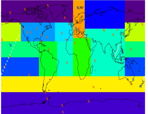
The control parameters chosen for the inversion are displayed in Tables 4 and 5.

They include the annual emissions of CO and NO_x over large geographical areas and

10

for diff_{erent broad source categories: (1) anthropogenic emissions of CO and NO}_x

in 8 regions (see Fig. 5) (2) NOx emissions from ships (3) biomass burnt in forest

and savanna fires in 4 regions (4) biomass burning emission factors for CO and NO_x

(5) natural emissions (vegetation, soils, lightning), and (6) CO and NOx deposition

velocities. 15

Note that in the case of vegetation fire emissions of CO and NO_x, changes between

a priori and optimized emissions result from the combined optimizations of biomass burnt and emission factors. For instance, the a posteriori savanna fire emissions of a compound are calculated by multiplying their a priori distribution by the exponentiated sum of the optimized control parameters corresponding to the region and to the species 20

emission factor:

G_sav(x, t)=_exp(_f_{E F,sav}₎

ℓ₄

X

ℓ=_ℓ 1

exp(f_ℓ)Φ_ℓ,sav₍_{x, t}₎ ₍₃₎

wheref_{E F,sav} is the optimized control variable corresponding to the savanna burning

(13)

ACPD

4, 7985–8068, 2004

Title Page

Tables Figures

◭ ◮

Back Close

Full Screen / Esc

Print Version

EGU

biomass burnt in savanna fires in four diff_{erent regions (cf. Table} ₅_{), and} Φ_ℓ,sav₍_{x, t}₎

are the a priori savanna fire emissions for the species considered.

The optimization algorithm proceeds as follows. In the first step, the model calculates

the state s(ti) for all ti, with fj=0,∀j. From this forward model simulation, the cost

function J : Rm→R, which quantifies the bias between the model prediction and the

5

observations, is calculated:

J(f)=_J_obs₍f)+_J_B₍f)

=1

2

p

X

i=₁

(H_i(f)−y_i)TE−1(H_i(f)−y_i)

+1

2(f−fB)

T_B−1

(f−f_B), (4)

J(f)=_J_obs₍f)+_J_B₍f)= 1

2

p

X

i=₁

(H_i(f)−y_i)TE−1(H_i(f)−y_i)+1

2(f−fB)

T_B−1

(f−f_B), (5) 10

whereE,Bare the matrices of error estimates on the observations and the emission

parameters, respectively,H_i=_π_◦_S_i_,_f_B _{is the first guess value for the control}

parame-ters (taken equal to zero as previously stated), and T means the transpose. The first

contribution,J_obs, measures the bias between the forward model predictions and the

chemical observations, whereas the second contribution,JB, is a regularization term

15

needed to ensure that the problem has a unique solution and to prevent a posteriori

emissions from being too diff_{erent from their initial guess values.}

We define the vectorǫoof observation errors and the vectorǫBof the a priori errors

on the emission parameters by the following relations:

ǫ_o=y−H(f_true), ǫ_B =f_true−f_B. (6)

20

Here, f_true is the best possible representation of the vector of control variables, and

(14)

ACPD

4, 7985–8068, 2004

Title Page

Tables Figures

◭ ◮

Back Close

Full Screen / Esc

Print Version

EGU includes errors produced during the observation process as well as errors on the

op-eratorH. Since it is supposed that the observation errors as well as the background

errors are uncorrelated, the matricesE and Bare diagonal; their diagonal terms are

the variances of the observation and a priori background errors, respectively. More precisely, the a priori background errors on the control parameters are defined as 5

f

∆_f_j = ∆_f_j_/Ω =q_B_jj_, ₍₇₎

where the values of∆_f_j _{are given in Tables} ₄ _and ₅_, _B_jj _{are the diagonal elements}

of the matrixB, andΩ _{is a regularization parameter adjusted to ensure an adequate}

weighting ofJ_obs and J_B in Eq. (5). Its value is initially taken equal to 5. The value

ofΩ_{will be modified in sensitivity tests presented in Sect.}₅_{. The values of}∆_f_j _range

10

from 0.5 for the best constrained emissions (i.e. anthropogenic emissions in Western Europe, North America and Oceania) to 1 for highly uncertain emission categories (e.g. natural emissions).

In the next step, the adjoint of the model (see next subsection) is used to calculate

the gradient of J with respect to the parameter vector f. Subsequently, applying a

15

suitable iterative descent algorithm onJ, which makes use of this gradient, we obtain

a new estimate for the parameter vector f. The latter is used as input for the next

simulation, and this algorithm continues untilJ reaches its minimum.

The gradient (∇J)f of the cost function with respect to the control variables is

calcu-lated as follows. By straightforward calculation, we obtain that ifI:Rm →Ris a scalar

20

function of the form:

I(x)= 1

2α(x)

T_Kα_(x)_, _∀_x_∈_Rm_, ₍₈₎

whereα is a diff_{erentiable vector function}_α _: _Rm_→_Rn_,_K_{a symmetric constant}_n_×_n

matrix, andT means the transpose, then the gradient (∇I)x is given by

(∇I)_x =₍_Dα)T_xK α(x). (9)

(15)

ACPD

4, 7985–8068, 2004

Title Page

Tables Figures

◭ ◮

Back Close

Full Screen / Esc

Print Version

EGU

Here (Dα)x, the derivative of α at x is viewed as a linear transformation R

m

→ Rn

(Jacobian matrix):

(Dα)x =

     

∂α₁

∂x1(x). . . ∂α₁

∂xm(x)

..

. ...

∂α_n

∂x1(x). . . ∂α_n

∂xm(x)

     

. (10)

Applying now Eq. (9) in the case of the cost function of Eq. (5), it is straightforward

that: 5

(∇J)f =

p

X

i=₁

(DH_i)T_fE−1(H_i(f)−y_i)+_B−1₍f −f_B) (11)

3.2. Adjoint code generation and minimizer

The cost function is an example of a complicated numerical algorithm consisting in a

composition of diff_{erentiable mappings. Let us now examine how the gradient of this}

function can be calculated, by using Eq. (11).

10

Let us consider the general algorithmA :Rm→Rn, which can be decomposed into

K ∈ N steps, A=_AK _◦_{. . .}_◦_A1_{, where} _Aℓ _: _Rnℓ−1_→_Rnℓ_, _Zℓ−1 _7→ _Zℓ_, _ℓ _{∈ {}₁_{, . . . , K}_}

are diff_{erentiable maps. Applying the chain rule of di}ff_{erentiation, we can write for the}

derivative ofAatX=_X₀_:

(DA)_X

0 =(DA

K₎

Z₀K−1◦. . .◦(DA2)Z₀1◦(DA1)X₀, (12)

15

where we have used the notationZ₀ℓ=₍_Aℓ _◦_{. . .}_◦_A1₎₍_X₀_{), 1}_≤_ℓ_≤_K_{, and the convention}

Z₀0=_X₀_{. For the computation of multiple matrix products like in Eq. (}₁₂_{), we might either}

(16)

ACPD

4, 7985–8068, 2004

Title Page

Tables Figures

◭ ◮

Back Close

Full Screen / Esc

Print Version

EGU operate in reverse mode, from the left to the right. Taking the adjoint (transpose) of

Eq. (12) we have:

(DA)T_X

0

=₍_DA1₎T

X₀◦. . .◦(DA K₎T

Z₀K−1. (13)

Therefore, the reverse mode in Eq. (12) operates in the direction of the forward mode

in Eq. (13). This is the reason why the reverse mode is known as adjoint mode. Now,

5

since

D(AK ◦. . .◦Aℓ)_Zℓ−1 0

= _D₍_AK _◦_{. . .}_◦_Aℓ+1₎

Z₀ℓ ◦(DA ℓ₎

Z₀ℓ−1, K ≥ℓ ≥1, (14)

we can write:

D(AK ◦. . .◦Aℓ)T_Zℓ−1 0

=₍_DAℓ₎T

Z₀ℓ−1◦ D(A

K _◦_{. . .}_◦_Aℓ+1

)T_Zℓ 0

. (15)

This means that the derivative (DAℓ)T

Zℓ−1 0

of theℓth component ofAallows us to

calcu-10

late the derivative of the compositionAK ◦. . .◦Aℓ (k−ℓ terms) from the derivative of

the compositionAK ◦. . .◦Aℓ+1(k−ℓ−1 terms). Based on Eq. (15), we can calculate

the adjoint (transpose) of the model matrix, needed to derive the gradient of the cost

function of Eq. (11), for all algorithm stepsℓ.

In our case, the adjoint model is derived directly from the numerical code of the IM-15

AGES model. This code, viewed as a composition of functions, is diff_{erentiated by}

applying the chain rule, as previously described. Since application of the adjoint model reverses the execution order, the backward in time calculation requires the knowledge of the model state at each time step. For this reason, trace gases concentrations are stored on disk at every time step in the forward run (totalling approximately 14GB, 20

when the model time step is equal to 1 day). Using this checkpointing scheme, the adjoint model reads these concentrations, and thus, long recomputations are avoided.

The adjoint code is implemented using the automatic diff_{erentiation software TAMC}

(17)

ACPD

4, 7985–8068, 2004

Title Page

Tables Figures

◭ ◮

Back Close

Full Screen / Esc

Print Version

EGU

programming eff_{ort, due to redundant recomputations generated by the compiler; the}

elimination of these recomputations has involved important modifications of the forward and adjoint codes. Using 8 processors on a SGI Origin 3400 Batch server, the runtime is 15 minutes for a complete simulation of the forward model and 1 h for the adjoint one. The cost function and the derivatives calculated in the forward and adjoint mod-5

els respectively, are used as inputs in the minimization subroutine M1QN3 developed byGilbert and Lemar ´echal(1989). This minimizer solves unconstrained minimization problems using a variable storage quasi-Newton method, where the inverse Hessian

matrix is updated by the inverse BFGS formula (see for exampleNocedal and Wright,

1999, and the next subsection). The computation of the cost function and its

gradi-10

ent is then performed iteratively. The convergence criterion used in the optimization runs is that the norm of the gradient of the cost function after minimization is reduced by a factor of 1000 with respect to the initial one. In most optimization runs, how-ever, the minimization procedure has been continued after the convergence criterion was reached. These additional iterations were found to result in negligible changes, 15

however.

3.3. A posteriori error estimation

The relation between the inverse Hessian matrix of the cost function at the minimum and the a posteriori error estimates of the control parameters has been discussed in

Thacker(1989) andRabier and Courtier(1992). This result is briefly presented below, 20

and adapted to the case of the IMAGES model. Next, the estimation of the a posteriori errors using the inverse BFGS algorithm and the DFP formula will be discussed.

Using the fact that in a euclidean space the Hessian matrix of a (scalar) function can be obtained as the derivative of the gradient of the function, we can write for the Hessian of the cost function:

25

Hess(J)_f =_[_D₍_∇_J_)]_f =

p

X

i=1

(D2H_i)T_fE−1(H_i(f)−y_i)+

p

X

i=1

(18)

ACPD

4, 7985–8068, 2004

Title Page

Tables Figures

◭ ◮

Back Close

Full Screen / Esc

Print Version

EGU It is clear that, when the model is linear, the second order term of the Hessian is zero.

As long as the model is not too far from being linear, the Hessian of the cost function

is well approximated by the first order term of Eq. (16) and the second derivative term

is ignored.

The linearity assumption has been checked by evaluating the diagonal elements of 5

the first and second order terms of the Hessian by finite diff_{erences on the forward}

model results. The second order term, which takes the non-linearities into account, is indeed found to be about one order of magnitude smaller than the first order term. Due to the expensive computational cost required in these calculations, this comparison is

performed for only one optimization run (case study A, see Table9). For the rest of this

10

work, we will proceed with the linearized Hessian matrix.

By putting now (∇J)f=0 in Eq. (11) and using Eq. (6), and taking into account that

the observation and background errors are uncorrelated, we find that the expectation

valueE[(f −f_true)(f −f_true)T]=_E˜_{, which represents the a posteriori error covariance}

matrix, is related to the Hessian of the cost function through the following relation: 15

˜

E=

p

X

i=1

(DH_i)T_fE−1(DH_i)f +B−1

−1

=_Hess₍_J₎−1

f . (17)

In the present study, two algorithms have been used in order to approximate the true

Hessian matrix, based on the inverse BFGS and DFP updating formulas (e.g.Nocedal

and Wright,1999). Both algorithms start with an initial approximation of the inverse

Hessian matrix (IH)₀ (usually chosen to be a diagonal matrix, e.g., the identity matrix

20

or the Hessian of the background term in the cost function,B) and combine the most

recently acquired information about the objective function with the existing knowledge

embedded in the current Hessian approximation. Given a sequence s_k=f_k+1 −fk

andy_k=₍_∇_J₎_f

(19)

ACPD

4, 7985–8068, 2004

Title Page

Tables Figures

◭ ◮

Back Close

Full Screen / Esc

Print Version

EGU

Hessian matrixIHcan be generated either by the inverse BFGS update formula:

(IH)_k+1=(IH)k+

s_ksT_k

yT_ks_k −

(IH)kyksTk

sT_ky_k −

s_kyT_k(IH)k

yT_ks_k

+sky

T

k(IH)kyksTk

sT_ky_ksT_ky_k , (18)

or by the DFP formula:

(IH)k+1=(IH)k+

s_ksT_k

yT

ksk

−(IH)kyky

T k(IH)k

yT

k(IH)kyk

. (19)

Both updates generate symmetric and positive definite approximations whenever 5

the initial approximation (IH)₀is positive definite andsT_ky_k>0 (e.g.Nocedal and Wright,

1999).

Iterative application of the inverse BFGS or DFP formulas (Eqs.18,19) on the

vec-torsf_kand (∇J)_f_k calculated in the minimization procedure, provides an approximation

of the inverse Hessian matrix. This estimation for the inverse Hessian is evaluated 10

against finite diff_{erence calculations performed on the adjoint model. In order to obtain}

reliable results, the Hessian is calculated for diff_{erent perturbations around the initial}

parameter vector. Although generally far too computationally demanding, this method

has been applied in the case studies A and B of Table9. The results will be compared

and discussed in Sect. 7. The square roots of the diagonal elements of the inverse

15

Hessian matrix correspond to standard errors for each control parameter of the model;

the off_{-diagonal terms represent correlations between pairs of control parameters.}

4. Observations

Three diff_{erent types of observations are used as constraints in the case studies}

pre-sented in the next section: ground-based measurements of CO mixing ratios and CO 20

vertically integrated columns, NO2 tropospheric columns retrieved from a satellite

(20)

ACPD

4, 7985–8068, 2004

Title Page

Tables Figures

◭ ◮

Back Close

Full Screen / Esc

Print Version

EGU addition, aircraft campaign measurements of CO are used as independent

observa-tions in order to evaluate the inversion results. These observaobserva-tions are decribed below.

4.1. Ground-based measurements

a)CO mixing ratios are provided by the NOAA/CMDL global sampling network (Novelli

et al.,1998,2003) and made freely available via ftp (ftp://140.172.192.211/ccg/co/flask/

5

event). Data consist of CO volume mixing ratios, sampling and analysis information for

each flask sample, for 47 sampling locations (described in Table 6) and 2 shipboard

programs, the Pacific Ocean Cruise and the South China Sea Cruise. The site locations

(shown in Fig. 8) have wide latitudinal as well as longitudinal coverage, although a

majority of sites are located in the northern mid-latitudes. As the CMDL network was 10

originally intended to monitor the atmospheric composition in unpolluted conditions, most sites are located in the remote atmosphere.

In the present study, continental sites situated above 2500 m a.s.l. (Plateau Assy, Niwot Ridge, Mt. Waliguan, Assekrem) are not taken into account in the inversion, since the model resolution does not allow to account for topographical heterogeneities. 15

Furthermore, when measurements from neighbouring stations present similar concen-trations and seasonal features (e.g. Alert, Svalbard, Mould Bay), then, to avoid redun-dancy, we consider data from only one station in the calculation of the cost function

(see Table6). For instance, among high-latitude southern hemisphere stations (Tierra

Del Fuego, Palmer, Syowa, Halley, South Pole), only data from Tierra Del Fuego station 20

have been taken into account for the inversion.

Contrary to previous inversion studies based on the same measurements (P ´etron

et al.,2002), we take into account CMDL data representing non-background conditions

(i.e., samples contaminated due to winds blowing from the direction of areas likely to produce CO), since the model introduces no filtering. However, exceptional events with 25

concentrations more than three times greater than the mean value calculated over the period 1997–2001, are considered exceptional, and are excluded from further analysis.

(21)

com-ACPD

4, 7985–8068, 2004

Title Page

Tables Figures

◭ ◮

Back Close

Full Screen / Esc

Print Version

EGU bines the standard deviation of the measurements around their monthly means with an

assumed representativity error of 10%:

σ_obs2 =₍1 n

n

X

j=1

c2_j −c¯2)+₍₀_.₁₀_·c¯)2, (20)

wherec_j are the detrended monthly concentrations, ¯ctheir monthly averages, and n

their number. The actual errors on the flask measurements are believed to be small, 5

on the order of a few ppb (Novelli et al.,2003) and are therefore neglected. The first

term of Eq. (20) corresponds to a variability error associated with the variability of the

observations around their monthly averages. It is usually small when the number of

measurements is suffi_{ciently large (}_n_≫_{10). It is found to be most significant at the}

shipboard locations in the South China sea, where n is small and variability is large

10

due to the proximity of large emission sources.

b) The CO vertical column abundances are provided by the column-measuring

sta-tions listed in Table7. Ground-based FTIR (Fourier Transform InfraRed) instruments

are used in all cases. Part of the data (for Ny-Alesund, Kitt Peak, Mauna Loa and Wol-longong) is publicly available via the Network for the Detection of Stratospheric Change 15

(NDSC) web site (http://www.ndsc.ncep.noaa.gov). The data for the NDSC stations of

Jungfraujoch and Lauder were provided byBarret et al.(2003) andJones et al.(2001),

respectively. The CO columns at St Petersburg were provided by Makarova et al.

(2001). The error associated to the data is calculated as in the case of CMDL stations,

except that the error on the column retrieval by FTIR (on the order of 10%) must also 20

be taken into account. The representativity error is therefore replaced by a 15% error which includes both the representativity and measurement errors.

4.2. Satellite observations

This study uses an improved version (V1b)(Richter et al.,2003) of the tropospheric NO2

columns retrieved from measurements by the GOME spectrometer aboard the ERS-25

(22)

ACPD

4, 7985–8068, 2004

Title Page

Tables Figures

◭ ◮

Back Close

Full Screen / Esc

Print Version

EGU

method (TEM) was used in Richter and Burrows (2002) in order to separate

tropo-spheric and stratotropo-spheric contributions of the total measured NO₂column. It assumes

that the stratospheric NO2column is longitudinally constant, and that the tropospheric

NO2 column amounts above a Pacific sector between 170◦W to 180◦W can be

ne-glected. The first assumption is reasonable at low latitudes; however, close to the 5

poles, longitudinal variations cannot be neglected and artifacts are introduced in the tropospheric columns. In version 1b, the subtraction of the stratospheric column uses

the stratospheric NO₂fields calculated by the SLIMCAT model, as described inRichter

et al. (2003). This procedure reduces, but doesn’t suppress, the errors associated to

stratospheric variations. The next step to the data analysis is the correction of the tro-10

pospheric light path using the airmass factor calculation. In version 1b, these airmass

factors are estimated using the the tropospheric NO2 distributions from the MOZART

model. Due to the sun-synchronous orbit of ERS-2, measurements of GOME are per-formed around the same local time, 10:30 LT.

GOME measurements for the year 1997 are used in this study (http://www.

15

doas-bremen.de/gome no2 data.htm), gridded at the resolution of the model. The

Figs.6and7display the NO₂column distribution for March and September. To account

for the fact that measurements take place at 10:30 LT, the diurnally averaged NO2

con-centrations calculated by the model are multiplied by a correcting factor expressing the

ratio of the NO₂concentration at 10:30 LT to the average NO₂concentration. This ratio

20

is calculated from the full diurnal cycle calculations, which are performed off_-line.

The uncertainties on the tropospheric NO2 columns derived from GOME

measure-ments are related to the stratospheric subtraction procedure, to the calculation of

air-mass factors (i.e. on the NO2vertical profile, surface albedo, and aerosol loading), and

to the presence of clouds (seeRichter and Burrows,2002, for a detailed error analysis;

25

error estimation for a particular case has been done byHeland et al.(2002)). In order

to calculate the NO2 contribution to the cost function (Eq. 5), we take the

observa-tion errors to be equal to the maximum value of 5·1014molecule/cm2and 20% of the

(23)

ACPD

4, 7985–8068, 2004

Title Page

Tables Figures

◭ ◮

Back Close

Full Screen / Esc

Print Version

EGU

model errors (i.e. errors associated with to the design of the operatorH); their

quan-tification stands beyond the scope of this work. Due to the short lifetime of the NO_x

family, the NO2concentrations predicted by the IMAGES model in remote areas (e.g.

the oceans) are likely to be less reliable than in the vicinity of the emission regions. Therefore, only continental pixels are considered in the calculation of the cost function. 5

Furthermore, snowy pixels and pixels located poleward of 60◦ are rejected, since the

NO2retrieval is expected to be more uncertain in these areas.

4.3. Methane lifetime

Loss of atmospheric methane is dominated by its reaction with the hydroxyl radical (OH) in the troposphere. The loss term can be deduced from methylchloroform budget 10

studies (see for examplePrinn et al.,2001;Krol and Lelieveld,2003). The tropospheric

methane lifetime due to the reaction with OH is defined as the quotient of the total bur-den by the tropospheric loss by OH. In this study, the TAR recommended OH value is

used (IPCC,2001). This value is equal to 9.6 yr and is scaled from a methylchloroform

OH lifetime of 5.7 yr. An additional term of the form 15

JCH4=A(τCH4−9.6)2 (21)

is then added to the cost function, which quantifies the discrepancy between the tropo-spheric methane lifetime calculated by the model and the aforementioned value. In this

equation,τCH4 is the tropospheric methane lifetime calculated by the model (yrs), and

Ais a constant suitably adjusted in order to ensure that the methane lifetime constraint

20

is eff_{ective (}_A=₅_·₁₀3_).

4.4. Aircraft campaigns

Tropospheric data from a number of aircraft campaigns compiled by Emmons et al.

(2000) are used as independent observations to be compared to the optimized

con-centrations of carbon monoxide. The observations are averaged onto a 5◦×5◦

hori-25

(24)

ACPD

4, 7985–8068, 2004

Title Page

Tables Figures

◭ ◮

Back Close

Full Screen / Esc

Print Version

EGU data sets (number of measurements, minimum, maximum, mean, standard deviation)

can be accessed through the data composites web site (http://acd.ucar.edu/∼_emmons/

DATACOMP/camp table.htm). For our purposes, CO measurements have been

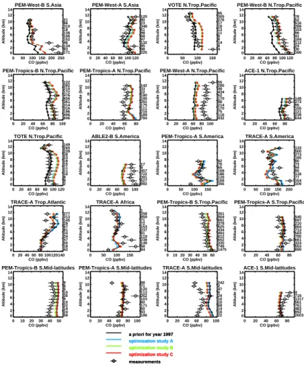
aver-aged over 14 large regions (Fig. 8). The model concentrations are averaged in the

same regions taking into account the location of the measurements and the number of 5

measurements at each location.

5. Inversion results

Five optimization studies were performed, using diff_{erent combinations of the}

obser-vational datasets described in the previous section, as shown in Table9. The target

period for the inversions is the year 1997. In these studies, CO (or CO and NO_x)

emis-10

sions are constrained using 1997 observations, the a priori emissions being provided

by the 1997 inventory summarized in Tables4and 5. In cases A, B and C the

back-ground errors on the control parameters are given by Eq. (7), with Ω=_{5. In order to}

test the stability of the results, two sensitivity studies have been conducted, where the background errors are halved (case B1) and doubled (case B2).

15

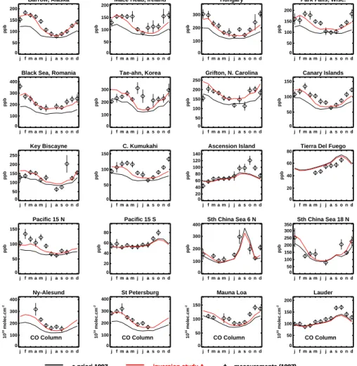
In Fig.9we compare the a priori and (in black) and optimized (in red) monthly

aver-aged CO measurements (mixing ratios and total columns) at selected sites. Only case

A results are shown, since the diff_{erences between cases A, B and C are found to be}

very small at these sites.

As seen on Fig.9, the optimization brings the model values much closer to the

mea-20

surements at mid- and high latitudes, compared to the a priori. The increase in CO mixing ratios, on the order of 10 ppbv in summer and 40 ppbv or more in late winter, is mainly achieved by increasing anthropogenic emissions at these latitudes, as will be discussed later in detail. However, a significant bias remains between the model and the data during springtime at most remote stations of the Northern Hemisphere, which 25

(25)

ACPD

4, 7985–8068, 2004

Title Page

Tables Figures

◭ ◮

Back Close

Full Screen / Esc

Print Version

EGU to a small but discernible improvement in springtime CO mixing ratios. As the

chem-ical lifetime of methane (8.63, 9.13 and 9.58 years in cases A, B and C, respectively) reflects primarily tropical OH concentrations, its constraint in case C has only a negli-gible influence on CO outside the Tropics. Model transport flaws are likely to explain most of the remaining discrepancies between observed and optimized mixing ratios. 5

The well reproduced concentration peak observed by the shipboard cruise at 6◦N from

August to October 1997 (also detected by GOME, as seen on Fig.10) is due to intense

Indonesian forest fires (e.g., Hauglustaine et al., 1999; Duncan et al., 2003), which

appear to be correctly represented in the 1997 emission inventory. A good agreement between optimized and observed CO columns is achieved in the Northern Hemisphere 10

(Ny-Alesund, St-Petersburg, Mauna Loa). However, the inversion has only a small im-pact on the calculated mixing ratios and columns at Southern high latitudes (Lauder, Wollongong, Cape Grim, Crozet and Tierra del Fuego). In this region, the model under-estimates CO columns, while overestimating the surface concentrations. This feature is consistent with the underestimation of vertical gradients at these latitudes seen in 15

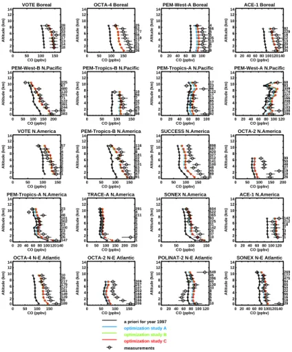
the comparisons with aircraft measurements (see Sect.6).

The inversion study A predicts an increase of the global surface emission flux of CO by 4%, whereas slight decreases are found in cases B and C (2% and 5%, resp.). The photochemical production of CO by methane and NMVOCs oxidation decreases in all

cases, by 1% in case A, 8% in B, and 11% in case C, as shown in Table 10. The

20

direct sources increase is mostly due to anthropogenic emissions over industrialized regions and countries in economical transition. More precisely, the largest increases occur over N. America (48% in A, 37% in B and C), Europe (24% in A, 16% in B and C), Former Soviet Union (168% in A, 145% in B, 151% in C), South Asia (29%, 23%, 25% in A, B, C resp.), and Far East (21% in A, 14% in B, C), with respect to their prior 25

values displayed in Table4. The diff_{erent inversions agree on a decrease of about 16%}

over Oceania.

The TAR recommended value for the total CO source of year 2000 amounting to

(26)

partic-ACPD

4, 7985–8068, 2004

Title Page

Tables Figures

◭ ◮

Back Close

Full Screen / Esc

Print Version

EGU ular the estimate in case B (2760 Tg CO/yr). Furthermore, anthropogenic emissions

derived by our analysis and the estimates proposed byIPCC(2001) are generally in

good agreement, e.g. over North America and Africa (their 137 against 124–134 Tg CO/yr, their 80 against 79–86 Tg CO/yr, respectively), with the exception of European

anthropogenic emissions, estimated at 109 Tg CO/yr byIPCC(2001), i.e., significantly

5

higher than our best estimates ranging between 54 and 58 Tg CO/yr.

A posteriori anthropogenic emissions over South America and Africa present a more significant increase in case B, compared to the other inversion studies. For instance, African emissions increase by 12% in B, and by 3% in A, while emissions over South America decrease by 3% in A, increase by 6% in B and remain constant in C. The 10

increase in Tropical CO emissions in case B appears to be necessary in order to

com-pensate for the higher photochemical sink of CO caused by increased Tropical NOx

emissions, as will be discussed further below.

The biogenic emissions of CO and NMVOCs are decreased by 11–20%. The poste-rior isoprene emissions amount to 504 Tg/yr in case A and 454 Tg/yr in case B, while 15

monoterpene emissions amount to 128 Tg/yr in A and 115 Tg/yr in inversion B. Biomass burning emissions of CO are decreased by 12–18% compared to their bottom-up value

(Table10). Savanna burning emissions decrease by a factor equal to 1.4 in A and 1.3

in B. Asian tropical forest burning emissions are reduced by 15–22%. On the other hand, extratropical forest burning emissions present an important increase (43% in A, 20

C, 50% in B) which might be partly driven by the model underestimation at Tae-ahn in

June–July (Fig.9). Whereas African forest burning emissions preserve their a priori

value in case study A, they increase significantly when GOME observations are con-sidered in the inversion (55% in B, 50% in C). Note that the magnitude of the latter two

sources being very small (Table5), these large relative changes predicted by the

inver-25

sions have only a small influence on the concentrations. As will be explained in Sect.7,

little confidence should be given to the results obtained on vegetation fire emissions, since their estimated a posteriori uncertainties remain quite large.

(27)

ACPD

4, 7985–8068, 2004

Title Page

Tables Figures

◭ ◮

Back Close

Full Screen / Esc

Print Version

EGU

by 14-17%, as described in Table11and illustrated in Fig.12. It is mostly due to

pro-nounced anthropogenic emission decreases over the Former Soviet Union (52%), the

Far East (36%), and Europe (27%). Although these changes bring the calculated NO2

columns closer to the observations during the summer over Europe and the Far East

(Fig.10), they also result in a significant underestimation in wintertime. The reasons

5

for this poor representation of the seasonal cycle of NO2 columns at mid-latitudes are

unclear.

Whereas in case A, the higher CO anthropogenic emissions lead to a decrease in OH abundances at mid- and high latitudes, amounting to 15–25% on annual average,

the NOx decrease at mid-latitudes in cases B and C brings OH at still lower levels at

10

these latitudes, on the order of 25–35%, as seen on Fig.13. The resulting longer CO

lifetime explains the weaker increases of CO anthropogenic emissions at mid-latitudes in cases B and C, compared to case A. This gives an example of how the chemical

interplay between NO_xand CO influences the inversion results.

Another example is provided by the decrease in biogenic CO and VOC emissions 15

noted in case B. This change is related to the underestimation of NO2columns in the a

priori simulation over continental tropical regions during the wet season (Fig.10), which

lead to an increase in NOx emissions over those regions: anthropogenic emissions

over Africa increase by 19%, and the tropical soil emissions almost double, reaching

10.5 Tg N. In an attempt to further increase NO2 abundances in the Tropics, the

in-20

version scheme provides decreased biogenic VOC emissions, because the formation of nitrates and PAN associated with the oxidation of biogenic VOCs (in particular

iso-prene) is a significant sink of NOxover source regions (Chen et al.,1998). As a result,

an increase by 30% in oceanic CO emissions is also predicted, which partly compen-sates for these decreased biogenic emissions and for the substantial increase in OH 25

levels in the Southern Tropics, as seen on Fig.13. A sensitivity test, where the isoprene