www.atmos-meas-tech.net/8/1901/2015/ doi:10.5194/amt-8-1901-2015
© Author(s) 2015. CC Attribution 3.0 License.
Observing crosswind over urban terrain using scintillometer and
Doppler lidar
D. van Dinther1, C. R. Wood2, O. K. Hartogensis1, A. Nordbo3, and E. J. O’Connor2,4 1Meteorology and Air Quality Group, Wageningen University, Wageningen, the Netherlands 2Finnish Meteorological Institute, Helsinki, Finland
3Department of Physics, University of Helsinki, Helsinki, Finland 4Department of Meteorology, University of Reading, Reading, UK
Correspondence to:C. R. Wood ([email protected])
Received: 28 April 2014 – Published in Atmos. Meas. Tech. Discuss.: 1 July 2014 Revised: 26 March 2015 – Accepted: 6 April 2015 – Published: 24 April 2015
Abstract.In this study, the crosswind (wind component per-pendicular to a path,U⊥) is measured by a scintillometer and
estimated with Doppler lidar above the urban environment of Helsinki, Finland, for 15 days. The scintillometer allows acquisition of a path-averaged value ofU⊥(U⊥), while the
lidar allows acquisition of path-resolvedU⊥ (U⊥(x), where
x is the position along the path). The goal of this study is to evaluate the performance of scintillometer U⊥ estimates
for conditions under whichU⊥(x)is variable. Two methods
are applied to estimateU⊥from the scintillometer signal: the
cumulative-spectrum method (relies on scintillation spectra) and the look-up-table method (relies on time-lagged correla-tion funccorrela-tions). The values ofU⊥of both methods compare
well with the lidar estimates, with root-mean-square devia-tions of 0.71 and 0.73 m s−1. This indicates that, given the data treatment applied in this study, both measurement tech-nologies are able to obtain estimates of U⊥ in the complex
urban environment. The detailed investigation of four cases indicates that the cumulative-spectrum method is less sus-ceptible to a variableU⊥(x)than the look-up-table method.
However, the look-up-table method can be adjusted to im-prove its capabilities for estimatingU⊥under conditions
un-der for whichU⊥(x)is variable.
1 Introduction
The general application of a scintillometer in micrometeorol-ogy is obtaining path-averaged surface fluxes (among others De Bruin, 2002; Meijninger et al., 2002a, b). The path can
range from a few hundred metres to a few kilometres depend-ing on the type of scintillometer used (De Bruin, 2002). In this study, the focus is on obtaining the path-averaged cross-wind from a scintillometer (among others Briggs et al., 1950; Wang et al., 1981), where the crosswind (U⊥) is defined as
the wind component perpendicular to the scintillometer path. By obtaining a path-averaged value ofU⊥(U⊥) instead of a
point measurement, a scintillometer is more suitable to vali-date wind fields calculated by models – given the resolution of numerical weather prediction models (∼10 km). Further-more, point measurements can more easily be biased than path-averaged values, especially for urban areas at heights within about 2–3 times the canopy-layer depth (the canopy layer is typically defined as the average building height).
From scintillometer data, one can obtainU⊥ from either
the scintillation power spectrum (S11(f ), wheref is the fre-quency) (van Dinther et al., 2013) or the time-lagged corre-lation function (r12(τ ), whereτ is the time lag) (among oth-ers Briggs et al., 1950; Poggio et al., 2000; van Dinther and Hartogensis, 2014). Validation attempts ofU⊥have mainly
taken place at flat grassland sites (Poggio et al., 2000; van Dinther et al., 2013). At such sites,U⊥is assumed to be
uni-form along the scintillometer path. Furthermore, there is also a need for scintillometerU⊥ in more complex areas, such
as mountain environments (Poggio et al., 2000) and urban environments (above the River Thames in London in Wood et al., 2013c). Ward et al. (2011) studied the influence of a variableU⊥field along the path (U⊥(x), wherexis the
parameter estimates rather than onU⊥estimates. TheU⊥(x)
fields used in their study were synthetic. In the present study, the focus is on the influence of a measured variableU⊥(x)
on theU⊥estimate of a scintillometer.
The measurements investigated in this study are taken in the urban environment. In such an environment, the wind speed and direction are spatially variable (Bornstein and Johnson, 1977), making it a suitable environment to study the influence of a variableU⊥(x)on the scintillometer
esti-mates ofU⊥. Key to this study are measurements of the
vari-ability of U⊥(x)that are estimated by a scanning Doppler
lidar. In this experiment the lidar was configured in a hori-zontal scan pattern, in order to estimate the horihori-zontal wind speed and wind direction along the scintillometer path using a duo-beam method (Wood et al., 2013c).
The measurements were taken in Helsinki, Finland, as part of the Helsinki Urban Boundary-layer Atmosphere Network (Helsinki UrBAN; Wood et al., 2013a, http://urban.fmi.fi). The spatial and temporal variability of U⊥(x) induced by
buildings poses challenges for both the lidar and the scintil-lometer technologies: (i) the lidar, since one assumes homo-geneity of the wind field within each range gate (sampling bin) for both beams in the lidar duo-beam pair, and (ii) the scintillometer, since bothS11(f )andr12(τ )used in theU⊥
-retrieval algorithms are influenced by a variable U⊥(x),
al-though the algorithms do not take this into account (van Dinther et al., 2013; van Dinther and Hartogensis, 2014). We are, therefore, working at the limit of both measurement tech-nologies.
The main goal of this study is to investigate the perfor-mance of the scintillometer to measureU⊥in conditions for
whichU⊥(x)is variable. In order to do so, estimates from
the scintillometer ofU⊥are compared to estimates from the
lidar. However, also for the lidar, heterogeneous wind con-ditions are challenging. Therefore, before the scintillometer and lidarU⊥estimates are compared to each other, the
appli-cability of the lidar to estimateU⊥(x)is investigated by
com-paring with sonic-anemometer measurements. Lastly, four cases will be selected where lidar-estimated U⊥(x)values
are used to obtain the theoreticalS11(f )andr12(τ ), from the models given by Clifford (1971) and Lawrence et al. (1972), respectively. The influence of a variableU⊥(x)on the
theo-reticalS11(f )andr12(τ )gives insight into the robustness of the scintillometer methods to obtainU⊥.
2 Theory and methods 2.1 Scintillometry
A scintillometer comprises a transmitter and a receiver. Here, a large-aperture scintillometer is used and its transmitter emits near-infrared radiation, which is scattered by con-stantly changing eddies as it passes through the turbulent atmosphere. Hence, the intensity measured by the receiver
fluctuates on short timescales (∼1 s). For these timescales Taylor’s frozen-turbulence assumption is valid, makingU⊥
the only driver of changes in the eddy field.
The value ofU⊥can be obtained from the intensity
fluc-tuations (also referred to as scintillation signal) by either the scintillation power spectrum or time-lagged correlation func-tion. The benefit of the methods relying on r12(τ ) instead ofS11(f )is that also the crosswind direction (i.e. the sign ofU⊥) can be obtained fromr12(τ ). Another benefit is that
r12(τ ) can be determined over a short timescale (∼10 s), whileS11(f )needs to be determined over a longer timescale (∼10 min). On the other hand,r12(τ )needs to be obtained from a dual-aperture scintillometer, while scintillation spec-tra be obtained from every type of scintillometer.
In this study we use the cumulative-spectrum method to obtain U⊥ from S11(f )(van Dinther et al., 2013) and the look-up-table method to obtainU⊥fromr12(τ )(van Dinther and Hartogensis, 2014). A detailed description of the meth-ods is given in van Dinther et al. (2013) and van Dinther and Hartogensis (2014); a brief outline of the methods is given below.
2.1.1 Scintillation spectra
The scintillation spectrum (S11(f )) gives insight into which frequencies contribute to the variance of the scintillation signal. Clifford (1971) describes a theoretical model of the scintillation spectrum. Adjusting this model for the large-aperture scintillometer gives (Nieveen et al., 1998)
S11(f )=16π2k2 1 Z
0
∞
Z
2πf/U⊥(x)
(1)
Kφn(K)sin2
K2Lx(1−x) 2k
h
(KU⊥(x))2−(2πf )2
i−1/2
2J1(0.5KDRx) 0.5KDRx
2
2J1(0.5KDT(1−x)) 0.5KDT(1−x)
2 dKdx,
wheref is the frequency at whichS11 is representative, k is the wavenumber of the emitted radiation,K the turbulent spatial wave number,Lis the scintillometer path length,xis the relative location on the path,J1is the first-order Bessel function of the first kind,DRis the aperture diameter of the receiver,DTis the aperture diameter of the transmitter, and
φn(K)is the three-dimensional spectrum of the refractive in-dex in the inertial range given by Kolmogorov (1941). As can be seen in Eq. (1),U⊥(x)influences the scintillation
spec-trum. In fact, the scintillation spectrum shifts linearly across the frequency axis as a function ofU⊥. Therefore, by
obtain-ing a characteristic point in the spectrum,U⊥can be obtained
(van Dinther et al., 2013).
characteristic frequency points (fCS), which here are defined as the frequency points for which the cumulative spectrum equals 0.5, 0.6, 0.7, 0.8, and 0.9 (as in van Dinther et al., 2013). For each of these five points, a value ofU⊥is
deter-mined by
U⊥=CCS·fCS, (2)
where CCS is a unique constant which depends on the ex-perimental setup and scintillometer used. Derivation ofCCS is possible from the theoretical S11(f )(Eq. 1) by filling in values of U⊥ and assuming thatU⊥(x)is constant for the
five different frequency points. Subsequently, the five differ-ent U⊥ values are averaged to obtain one value ofU⊥ per
cumulative spectrum. In this study, we will investigate to what extent the assumption thatCCSis constant holds when
U⊥(x)varies. This investigation is carried out by means of
four cases for which theU⊥(x)estimates of the lidar are used
in Eq. (1) to obtain the theoreticalS11(f ). Therefore, Eq. (1) is not integrated for x over 0 to 1, but over the 136 range gates measured by the lidar (see Sect. 4.3). In this study, cu-mulative spectra are obtained over periods of 10 min. 2.1.2 Time-lagged correlation function
The value ofU⊥can be obtained from a dual-aperture
scin-tillometer (scinscin-tillometer with horizontally displaced beams) using r12(τ ). For a dual-aperture scintillometer, the two transmitters and receivers are in general displaced by only a small distance (∼10 cm). This small spatial difference means that the eddy field barely changes as the wind trans-ports it through one beam to the next (i.e. the frozen-turbulence assumption is not unreasonable). The signals of the two spatially separated scintillometer beams should thus be almost identical except for a time shift. This time shift is related to U⊥, and can be obtained fromr12(τ ). A theoret-ical model of the time-lagged covariance function (C12(τ )) is given by Lawrence et al. (1972), here including the large-aperture averaging terms of Wang et al. (1978):
C12(τ )=16π2k2 1 Z
0
∞
Z
0
(3)
Kφn(K)sin2
K2Lx(1−x) 2k
J0{K[s(x)−U⊥(x)τ]}
2J1(0.5KDRx) 0.5KDRx
2
2J1[0.5KDT(1−x)] 0.5KDT(1−x)
2 dKdx,
whereJ0 is the zero-order Bessel function of the first kind, ands(x)is the separation distance between the two beams at locationx. The theoreticalr12(τ )can be obtained by divid-ing the theoreticalC12(τ )by the theoretical C11(τ ), where
C11(τ )is obtained from Eq. (3) by takings(x)=0 (i.e. vari-ance of the signal).
In this study, we will use the look-up-table method to ob-tainU⊥fromr12(τ ). A look-up table is created with values of
the theoreticalr12(τ )(using Eq. 3) given a range ofU⊥
val-ues (resolution of 0.1 m s−1) and time-lag values (resolution of 0.002 s, equal to the measurement frequency of the scin-tillometer) (van Dinther and Hartogensis, 2014). Note that
U⊥(x)is assumed to be constant when creating the
look-up table. The estimate ofU⊥ is obtained by comparing the
measuredr12(τ )values to the theoreticalr12(τ )values of the look-up table. The theoreticalr12(τ )that has the best fit with the measuredr12(τ )thus yields the value ofU⊥.
The effects of having a variable U⊥(x) on r12(τ ) and thus onU⊥will be investigated by means of four cases (see
Sect. 4.3). For these four cases Eq. (3) is integrated over the 136 range gates given the different values for U⊥(x)
esti-mated by the lidar. In this studyr12(τ ), and thusU⊥, are
de-termined over intervals of 10 s. For the comparison between the scintillometer and lidar the 10 sU⊥values are
arithmeti-cally averaged to 10 min. 2.2 Doppler lidar
In this study, a HALO Photonics (Malvern, UK) Stream Line scanning Doppler heterodyne lidar is used. Full details of this type of lidar are described in Hirsikko et al. (2014) and only briefly summarized here. The lidar emits pulses of radi-ation at a wavelength of 1.5 µm; any backscattered radiradi-ation from aerosols is used to estimate wind in the atmosphere by assuming that aerosols are perfect tracers of the wind. The pulse repetition rate is 15 000 Hz; a 1 s ray is obtained from the accumulation of 15 000 pulses. In the returned sig-nal there is a Doppler shift, which enables calculation of the Doppler velocity, i.e. the velocity component in the direction in which the lidar beam is pointing (also referred to as radial or along-beam wind).
In this study, the crosswind component of the wind speed is needed in order to compare with scintillometer estimates. Note that also a sonic anemometer can yield valuable infor-mation about the local wind field above cities. However, in this study the interest is in the variability ofU⊥along a path,
which can be estimated from the radial Doppler velocities by applying the duo-beam method (Wood et al., 2013c). The method determines the horizontal wind speed and wind di-rection using trigonometric identities, from whichU⊥(x)can
be determined.
The duo-beam method relies, as the name implies, on two sets of measurements from the lidar: at two differ-ent azimuths (i.e. beam-pointing directions in the horizon-tal plane). A detailed description of this method is given in Wood et al. (2013c); a brief outline of the method is given here. The radial velocity (Vbg) for each range gate (g), as es-timated by the lidar, and beam number (b) is given by
θb, the two unknownsUgandφgcan be solved, by assum-ingV1g=V2g. FromUgandφg, the value ofU⊥can be
ob-tained for each range gate. It is implicit in this method that the wind field is homogeneous between the two lidar beams. Clearly this is not the case in the atmosphere, and one might expect the effects to average out well above buildings (e.g. often assumed so above the roughness sublayer; Roth, 2000; Kastner-Klein and Rotach, 2004). But at heights within, say, 2–3 mean building heights, there will inevitably be error, per-haps including bias, caused by this implicit assumption.
The fixed resolution of the radial wind (of 0.023 m s−1) also limits the duo-beam method; i.e. in general as the beam separation becomes infinitesimally small, so does the need for accuracy to become infinitesimally fine. Hence, a key drawback of the method is that, when winds are nearly par-allel to the path, winds cannot be estimated correctly.
3 Experimental setup
The measurements investigated in the present study were taken from 1 to 15 October 2013. The measurement devices used in this study are a scintillometer, a Doppler lidar, and two sonic anemometers. The layout of the measurement de-vices is given in Fig. 1.
The scintillometer used in this study is a BLS900 (Scin-tec, Rottenburg, Germany) running with SRun software ver-sion 1.09. Note that in this study the output ofU⊥, as given
from SRun, is not used. The BLS900 is a scintillometer with two transmitters and one receiver. Raw signal intensi-ties were measured and stored at a frequency of 500 Hz. The setup of the scintillometer is the same as that of other recent Helsinki scintillometer work (Wood et al., 2013b). The scin-tillometer measured over a path of 4.2 km. The transmitter unit was placed on a roof section of Hotel Torni at a height of 67 m, while the receiver was placed on a roof near the so-called SMEAR-III-Kumpula station at a height of 52.9 m (see Fig. 1). The surrounding areas have average building heights of 24 and 20 m, and zero-plane displacement heights of 15 and 13 m, at the transmitter and receiver, respectively (Nordbo et al., 2013). The orientation of the scintillometer was nearly north–south (17◦); therefore, the wind was nearly perpendicular to the scintillometer path when it was blowing from the east or west. In this study,U⊥is defined as positive
when the wind is blowing from the west into the path. The lidar was placed at a height of 45 m near the receiver of the scintillometer. Each ray lasts for 1 s and is repeated every 4 s. The lidar’s operational schedule only allowed two azimuth angles for this study (174 and 196◦) within each 5 min; see Fig. 1. This pair was wider apart than desired, due to line-of-sight issues. The elevation of the beam was 0.45◦. The lidar data are given in a series of 30-m range gates cen-tred at distances 105–9585 m from the instrument, but data were only needed until 4155 m (i.e. 136 range gates corre-sponding to the 4.19 km length of the scintillometer path).
24.9 24.92 24.94 24.96 24.98 60.14
60.15 60.16 60.17 60.18 60.19 60.2 60.21 60.22
Longitude [°E]
Latitude [
°
N]
(a)
4 3 2 1 00 20 40 60 80 100
><
Distance [km]
Height [m]
(b)
Anemometer North Anemometer South Lidar beams Scintillometer path Building maximum Building average Ground
Figure 1. (a)Experimental setup with the locations of the instru-ments in Helsinki indicated, including Doppler lidarbeam azimuths
of 174 and 196◦; shading is buildings/roads (white), grass/trees
(green), and water (blue) (land cover data source: HSY, SeutuCD);
the city centre is roughly the lower half of the map area.(b) A
cross section (height m a.s.l.) of the scintillometer beam and lidar
196◦beam; average building height and maximum building height
are with respect to±250 m laterally of the 196◦ beam (building
height data source available at https://sui.csc.fi/applications/paituli/ infra.html).
However – given the atmospheric aerosol loading, sensitiv-ity of the instrument, and integration times – sometimes not enough signal returned from the farthest gates and therefore resulting in a limited range of the data. In order to compare the lidar estimates withU⊥ estimates of the scintillometer,
two of the lidar estimates were averaged. Therefore,U⊥
es-timates of the lidar were available intervals of 10 min. A 3-D sonic anemometer was located at 75 m height (near the scintillometer transmitter, denoted here as “Anemome-ter South”) and another at 60 m (near the receiver, denoted here as “Anemometer North”); see Fig. 1. Due to the mast mounting, the wind directions are more uncertain for 0– 50◦ for Anemometer North and 50–185◦ for Anemometer South. Fortunately, the wind directions during the measure-ment period were mainly 210–350◦. For more details of the anemometer setup see Järvi et al. (2009) and Nordbo et al. (2013). The value ofU⊥measured by each of the
anemome-ters was added to the beginning and the end of the lidar-path estimates, giving a more complete data sample ofU⊥(x)
along the path. The estimates ofU⊥(x)were path-averaged
according to the scintillometer path-weighting function given by Wang et al. (1978) for fair comparison withU⊥estimated
by the scintillometer. In cases of missing U⊥(x)data, the
path-weighting factors were scaled to a total of 100 % in order to calculate the estimate ofU⊥ from lidar data. Note
the comparison between lidar and scintillometer, an arbitrary requirement was that at least 50 % ofU⊥(x)of the lidar data
were available along the scintillometer path.
4 Results and discussion
4.1 Doppler lidar path-resolved crosswinds
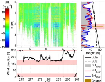
For the lidar, the urban environment is challenging, since the duo-beam method assumes a homogeneous wind field at each range-gate distance. This assumption will be violated to an unknown degree as the pair of beams diverges. How-ever, lidar is probably the only device which can measure the variability of the wind field along a beam. One other, al-beit unrealistic, alternative might be to measure the cross-wind along a path using multiple anemometers, but this will be a very challenging setup in the urban environment. How-ever, to ensure the quality of the lidar crosswind estimations, conditions are identified for which the lidar differs from the Anemometer South measurements. We evaluate the differ-ence between U⊥(x) estimated by the lidar and U⊥
mea-sured by Anemometer South, to see the impact of the wind direction and building height (see Fig. 2). Note that a per-fect agreement between the lidar and anemometer estimates is not expected, since the measurement locations are differ-ent. In this paper we only compare Anemometer South to the lidar, but comparing Anemometer North gave similar results (not shown here). The first 10 range gates of U⊥ of the
li-dar compared well with that measured by Anemometer South for the time-period studied, with root-mean-square deviation (RMSD) values of 0.57 m s−1. Hirsikko et al. (2014) showed for the same experimental setup, but a different time period, a RMSD of 0.53–0.67 m s−1for the Doppler velocity between lidar and sonic anemometer.
It should be noted that the sign ofU⊥(x)is determined by
the wind direction estimated by the lidar. When the wind is nearly parallel to the path, a small error in the estimated wind direction can result in an error of the sign of U⊥(x). The
wind directions for which the wind is nearly parallel to the path (167–227 and 347–47◦) are denoted in light-red shading in the lower figure panel (Fig. 2). It can clearly be seen that there is a substantial difference between lidar and anemome-ter data for these wind directions, especially when the wind is blowing from 200 to 227◦. Even sign changes of the
dif-ference are observed. The winds from the 200–227◦
direc-tions are also strong (>5 m s−1). Therefore, the correspond-ingU⊥(x)values are still moderate (absolute up to 3 m s−1)
for these wind directions. A small error in the wind direction can therefore result in a sign change of a moderateU⊥(x),
which is indeed what we see in Fig. 2. Also for the wind di-rection 347–46◦ there is a clear difference betweenU⊥(x)
of the lidar andU⊥ of the anemometer, with differences up
to 10 m s−1. Whilst we might expect differences above the urban canopy layer, to have such large differences for
hun-Figure 2.The upper left panel shows the difference inU⊥estimated by the Doppler lidar duo-beam method compared with Anemome-ter South (colour-bar, Doppler lidar minus sonic anemomeAnemome-ter) as a function of lidar beam distance (resolution of 30 m) and time (reso-lution of 10 min, DOY: day of year). A–D are cases (Table 1). The right panel shows the height (m a.s.l.) of the lidar beam and
build-ing height (BH)±25 m laterally underneath the paths (total, and
under beam with azimuth 174 and 196◦). When there are no
build-ings below the path, BH indicates the height of highest ground point or zero when it is over sea. The lower panel shows wind direction against DOY from Anemometer South.
dreds of metres seems unrealistic. That such large differences inU⊥(x)are unrealistic is also supported by Fig. 3, which
shows the estimates of the longitudinal wind component of the lidar along the path. These estimates seem slightly less heterogeneous along the lidar path. Perhaps the larger differ-ences ofU⊥(x)are caused by a breakdown of the
homogene-ity assumption required for the duo-beam method. Whatever the cause, in order to focus on when the method works, it was decided to exclude lidar values for which the wind direction is 167–227 and 347–46◦for the rest of the study (also when selecting the four cases).
The difference between lidar and anemometerU⊥ is also
large at 2000–2500 m along the lidar path (indicated in light red in Fig. 2 on the right). That the lidar estimates ofU⊥(x)
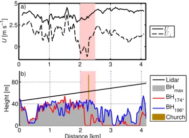
are unreliable for this part of the path is more clearly visible in Fig. 4, where the average horizontal wind speed (U) and the crosswind speed along the path as estimated by the lidar are shown. Note that in order to make this figure, the nearly parallel wind directions are excluded, as are times when the Doppler lidar data comprised less than 70 % of the total path. The value ofU⊥(x)even changes sign at the 2000–2500 m
section along the lidar path. The error inU⊥(x)for this
Figure 3. The Doppler wind component as estimated by the
Doppler lidar beam of 174◦, with lidar beam distance (resolution
of 30 m) and time (resolution of 10 min).
0 1 2 3 4
0 2.5
5 a)
U
[m s
−1
]
U U⊥
0 1 2 3 4
0 40 80
b)
Distance [km]
Height [m]
Lidar BH
max
BH174°
BH196°
Church
Figure 4. (a)Average horizontal wind speed and crosswind speed
estimated by the Doppler lidar. (b)The height (m a.s.l.) of the
li-dar beam and building height (BH)±25 m laterally underneath the
paths (total, and under beam with azimuth 174 and 196◦). When
there are no buildings below the path, BH indicates the height of highest ground point or zero when it is over sea.
distance from the lidar (see Fig. 1b). Although the church tower is somewhat to the east of the lidar path, it apparently has a significant influence on the wind field estimated by the lidar. The church alters the wind field of one of the lidar paths (196◦), while the other beam (174◦) does not encounter this alteration. Thus, the wind field sampled by the two lidar beams is not homogeneous, which causes problems for the duo-beam method. Therefore, we also excluded U⊥(x)
val-ues estimated by the lidar from 2000 to 2500 m for the eval-uation of scintillometer estimates with lidar estimates. How-ever, in order to evaluate the response of a variable U⊥(x)
onS11(f )andr12(τ ), and thus onU⊥estimated by the
scin-12:000 18:00 00:00 06:00 12:00
2 4 6
U⊥
B
L
S
[m
s
−
1]
a) Cum spectrum
Look-up table
12:000 18:00 00:00 06:00 12:00
2 4 6
U⊥
L
ID
A
R
[m
s
−
1] b)
12:000 18:00 00:00 06:00 12:00
2 4 6
Time[UTC] U⊥
S
on
ic
[m
s
−
1]
c) North
South
Figure 5.Time series ofU⊥as estimated by(a)the scintillometer,
(b)the Doppler lidar, and(c)the sonic anemometer for DOY 279
and 280.
tillometer, the four selected cases need the completeU⊥(x)
of the scintillometer path. Therefore, when selecting the four cases the value ofU⊥(x)had to be below 1.5·U⊥(of the lidar
estimates) for 2000 m≤x≤2500 m. The four cases selected are indicated in Fig. 2. These cases are spread over the mea-surement period and have differentU⊥values. The results of
the four cases are presented in Sect. 4.3.
Although the data for which the wind direction was 167– 227 or 347–46◦are excluded, as are the data at 2000–2500 m along the lidar path, there are still enough data left for the comparison between lidar and scintillometer. The exclusion resulted in 1288 10 min data points (60 % of the data) for the comparison between lidar and scintillometer.
Another issue which can influence the estimate ofU⊥(x)
of the lidar is temporal variability of U⊥(x). It is worth
briefly considering this issue. Temporal variability ofU⊥(x)
can result in biases and spread in the lidar estimate ofU⊥.
In order to investigate the temporal variability ofU⊥in these
data, the 10 min variance of 10 s estimates ofU⊥made by the
look-up-table method is calculated. The variance ofU⊥was
for 86 % of the time below 0.5 m s−1: a moderate temporal variability ofU⊥in these data.
4.2 Path-averaged crosswinds
In this section,U⊥obtained from the scintillometer is
0 2 4 6 8 0
2 4 6 8
|U⊥LIDAR|[m s−1]
|
U⊥
B
L
S
|
[m
s
−
1]
y = 0.72x + 0.96 R2 = 0.49 RMSD =0.73m s−1 # =1212
a)
−2 0 2 4 6 8
−2 0 2 4 6 8
U⊥LIDAR [m s−1]
y = 0.79x + 0.79 R2 = 0.56 RMSD =0.71m s−1 # =1286
b)
0.43052≤STD U<1 1≤STD
U<2 2≤STDU<3
3≤STDU<4
4≤STDU≤4.9856
Figure 6. (a)Crosswind 10 min averages estimated by the scintillometer (U⊥BLS) using the cumulative-spectrum method against Doppler
lidar crosswind (U⊥LIDAR).(b)Crosswind estimated by the scintillometer using the look-up-table method against lidar data. Both plots are
colour-coded with the lidar-derived path-weighted standard deviation of the crosswind along the 4.2 km path (see legend). The one-to-one lines are shown in thick black.
and the lidar beam causes a negligible difference in theU⊥
estimates. Assuming a neutral wind profile, the difference inU⊥ is merely 1.1 % (with the higherU⊥ estimate at the
height of the scintillometer), which suggests that the height difference between the two measurement devices should not influence the comparison. Note that this 1.1 % is only an ap-proximation; in reality the comparison is more complicated since part of the measurements are done just above the urban canopy layer where logarithmic wind profiles are not appli-cable.
Before looking into detail in the comparison between the lidar and scintillometer estimates of U⊥, we first show a
time series of U⊥ as estimated by scintillometer, lidar, and
sonic anemometers (Fig. 5). For the scintillometer estimates, it is clear that the cumulative-spectrum method and look-up-table method give very similar results. The lidar estimates of
U⊥fluctuates more strongly than both the scintillometer and
sonic anemometers. However, the lidar does capture the same pattern inU⊥as the scintillometer (especially on DOY 280
from 06:00 UTC onwards). For the sonic anemometers it is apparent that they do measure a different value ofU⊥, which
indicates that there is indeed spatial variability ofU⊥for this
instance.
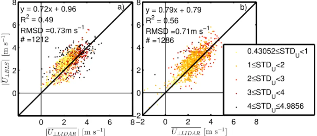
For the comparison of the lidar and scintillometer we first focus on the result of the cumulative-spectrum method (Fig. 6a). Note that the plots in Fig. 6 are coloured with the standard deviation averaged by the scintillometer path-weighting function (standard deviation of U⊥; i.e.
fluctua-tions of U⊥(x) in the middle of the path contribute more
to STDU⊥ than those at the ends of the path). Recall that
the sign of U⊥ is unknown with the cumulative-spectrum
method, and thus the absolute values ofU⊥are compared to
each other. The correlation betweenU⊥ of the
scintillome-ter and of the lidar gives confidence in the method, with a low RMSD of 0.73 m s−1. However, for a higher
path-weighted standard deviation along the scintillometer path (STDU⊥), more scatter occurs between the scintillometer
and lidar estimates. Only taking into account the data for which STDU⊥>2 m s−1 leads to anR2 value of 0.32 and
an RMSD of 0.86 m s−1. This higher scatter when STDU⊥>
2 m s−1 indicates the difficulty of estimating U⊥ when the
wind field is more variable along the path. An RMSD of 0.73 m s−1 is relatively low compared to other studies. For measurements in London (Wood et al., 2013c) for compa-rable wind conditions, horizontal wind speed RMSDs were found of 0.35 m s−1between two sonic anemometers on the same mast, 0.71–0.73 m s−1 between two sonic anemome-ters on different masts, and 0.65–0.68 m s−1 between lidar and sonic anemometers. ForU⊥, Wood et al. (2013c) showed
an RMSD of 1.12–2.13 m s−1between scintillometer and li-dar. For a flat grassland site, whereU⊥(x)can be assumed
to be rather homogenous, van Dinther et al. (2013) and van Dinther and Hartogensis (2014) showed RMSD values of quality-checked data of 0.41–0.67 m s−1 between a scintil-lometer and sonic anemometer for similarU⊥conditions
(ab-solute values are between 0 and 6 m s−1). Therefore, we can conclude that, despite the higher scatter for variableU⊥(x)
conditions, both measurement techniques seem able to obtain an estimate ofU⊥in this challenging environment.
In Fig. 6b, U⊥ obtained by the look-up-table method is
compared to the lidar estimates. Note that the following re-gression statistics are obtained when absolute U⊥ values
are considered: RMSD of 0.73 m s−1,y=0.76x+0.83, and
R2=0.53. Just like the cumulative-spectrum method, there is a clear correlation betweenU⊥ estimated by the
scintil-lometer and that estimated by the lidar. The regression statis-tics of the absoluteU⊥are similar with the same RMSD and
similar regression equation (although a slightly better fit for the look-up-table method). The scatter ofU⊥of the
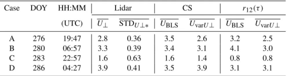
Table 1.Crosswind for the four cases estimated by the Doppler lidar and scintillometer (using either cumulative spectra, CS, or time-lagged
correlation function,r12(τ )).U⊥varU⊥is given by the theoretical CS andr12(τ )using the variableU⊥(x)estimated by the lidar.
Case DOY HH:MM Lidar CS r12(τ )
(UTC) U⊥ STDU⊥∗ UBLS UvarU⊥ UBLS UvarU⊥
A 276 19:47 2.8 0.36 3.5 2.6 3.2 2.5
B 280 06:57 3.3 0.39 3.4 3.1 4.1 3.0
C 283 22:57 1.6 0.63 1.6 1.4 0.8 0.8
D 286 04:27 3.9 0.41 3.5 3.9 3.1 3.1
that of the cumulative-spectrum method with an R2 value of 0.53 compared to 0.47. For the look-up table, the scatter is also higher (R2of 0.37 and RMSD of 0.88 m s−1) when
U⊥(x)is variable (STDU⊥>2 m s−1).
Overall, both scintillometer methods are able to obtain a similarU⊥ estimate as that of the lidar. This indicates that
both the lidar and scintillometer offer the potential to ob-tain an estimate ofU⊥over the complex urban environment.
However, remember that, in order to achieve these results, certain wind directions and a certain section of the path were not taken into account (see Sect. 4.1). The look-up-table method showed the best results, with the lowest RMSD and scatter.
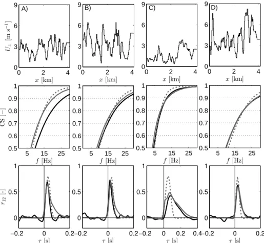
4.3 Variable crosswinds along the path
Four cases were selected to investigate the influence of a vari-ableU⊥(x)onS11(f )andr12(τ ): A, B, C, and D (see top panels in Fig. 7 and Table 1). As a measure of the variability ofU⊥(x), the weight-averaged standard deviation ofU⊥(x)
is normalized byU⊥(STDU⊥∗). For the four cases, the
the-oreticalS11(f )andr12(τ )are calculated using Eqs. (1) and (3), respectively.
We first focus on the cumulative scintillation spectra (CS, given in the middle panels of Fig. 7). Remember that the cumulative-spectrum method determines U⊥ from the
fre-quencies for which the CS is 0.5, 0.6, 0.7, 0.8, and 0.9. The spectra in Fig. 7 are zoomed such that the relevant points for this method stand out. For simplicity we abbreviate the cumulative spectrum obtained from the scintillometer as CSBLS, the cumulative spectrum obtained from Eq. (1) using
U⊥(x)of the lidar as CSvarU⊥, and the cumulative spectrum
obtained from Eq. (1) usingU⊥of the lidar as CSconstU⊥.
There is a difference between CSvarU⊥and CSconstU⊥for
all four cases. Therefore, the CS is indeed influenced by a variableU⊥(x)as was suggested by van Dinther et al. (2013).
Recall that, when a CS point shifts to a higher frequency, the retrieved value of U⊥ will be higher, and the other way
around (see Eq. 2). The CS points of 0.5, 0.6, and 0.7 lie at lower frequencies for CSvarU⊥than for CSconstU⊥, while
the 0.9 CS point lies at higher frequencies. CSBLS is more similar to CSvarU⊥than to CSconstU⊥, which indicates that
Eq. (1) is also applicable whenU⊥(x)is variable.
The results of applying the cumulative-spectrum method to CSBLS and CSvarU⊥ are given in Table 1. If the
as-sumption of the cumulative-spectrum methods – that CCS of Eq. (2) is constant – also holds for variableU⊥(x), then
the value ofU⊥ of the lidar should be identical to that of
UCSvarU⊥. For case D this is indeed true.
However, for case A, B, and C, UCSvarU⊥ is 0.2 m s −1
lower thanULiIDAR. Therefore, the assumption thatCCS is constant does not hold. However, the error that is made in
U⊥ is small (0.2 m s−1), which is due to the
cumulative-spectrum method calculatingU⊥ for five frequency points
and then averaging these to obtain one value for U⊥ (see
Sect. 2.1.1). For the 0.5, 0.6, and 0.7 CS points,UCSvarU⊥
is underestimated; while for the 0.9 CS point,UCSvarU⊥ is
overestimated. Therefore, applying a method with only one frequency point to obtainU⊥is more likely to have a higher
error. This makes the cumulative-spectrum method the most suitable method for obtainingU⊥fromS11(f )whenU⊥(x)
is variable, compared to other methods suggested by van Dinther et al. (2013). Alternatively, to obtainU⊥even more
reliably fromS11(f ) in variable U⊥(x)conditions, an
ap-proach similar to the look-up-table method can be applied. A look-up table can be created of the theoretical CS for differ-entU⊥values and also different variabilities ofU⊥(x).
Next we focus on the results of the look-up-table method, which relies onr12(τ )to obtainU⊥(given in the bottom
pan-els of Fig. 7). For all cases except case B, there is a sub-stantial difference in magnitude betweenr12varU⊥(τ )(grey
solid lines) andr12constU⊥(τ )(grey dotted lines). However,
the magnitude of r12(τ ) does not influence U⊥ obtained
by the look-up-table method, but the shape ofr12(τ ) does. The shape ofr12(τ ) also changes when U⊥(x)is variable:
it becomes wider. For cases C and D,r12varU⊥(τ )
resem-blesr12BLS(τ )clearly better thanr12constU⊥(τ ). This
resem-blance indicates that the theoretical model of Lawrence et al. (1972) (Eq. 3) can be used to obtainr12(τ )also given a vari-able U⊥(x). The fact that variable U⊥(x) causes a wider
r12(τ )can cause an underestimation ofU⊥obtained by the
scintillometer, since a widerr12(τ ) is normally associated with lowerU⊥ values. For the four cases selected in this
studyU⊥calculated fromr12varU⊥is indeed lower thanU⊥
0 2 4 0
3 6 9
x[km]
U⊥
[m
s
−
1]
A)
0 2 4
0 3 6 9
x[km]
B)
0 2 4
0 3 6 9
x[km]
C)
0 2 4
0 3 6 9
x[km]
D)
5 15 25 0.5
0.6 0.7 0.8 0.9 1
f[Hz]
C
S
[
−
]
5 15 25 0.5
0.6 0.7 0.8 0.9 1
f[Hz]
5 15 25 0.5
0.6 0.7 0.8 0.9 1
f[Hz]
5 15 25 0.5
0.6 0.7 0.8 0.9 1
f[Hz]
−0.2 0 0.2 0
0.5 1
τ[s] r12
[-]
−0.2 0 0.2 0
0.5 1
τ[s]
−0.2 0 0.2 0.4 0
0.5 1
τ[s]
−0.2 0 0.2 0
0.5 1
τ [s]
Figure 7.Four cases (A, B, C, and D): in the top panels the transect ofU⊥(x), in the middle panels the corresponding CS, and in the lower
panels the correspondingr12(τ ). The estimated CS andr12(τ )of the scintillometer are given as black solid lines, the theoretical CS and
r12(τ )givenU⊥(x)of the Doppler lidar are given as solid grey lines, and the theoretical CS andr12(τ )givenU⊥(x)=U⊥are given as
dashed grey lines.
obtained from r12(τ ). For case C and D, the error is high with a value of 0.8 m s−1. This high error is caused by the fact that for these two cases not only isr12(τ )lowered by the variableU⊥(x), but the peak inr12(τ )also changes location andr12(τ )becomes much wider due to the variableU⊥(x).
For these cases STDU⊥∗is also high with values of 0.63 and
0.41, respectively. Although the error with the lidar estimates is high for case C and D, the estimatedU⊥BLSof the look-up-table method are identical to that ofr12varU⊥(τ ). Therefore,
if the look-up table were expanded to also include a variable
U⊥(x)field, the results of the look-up-table method in a more
challenging environment could be improved. The underesti-mation ofU⊥given in the cases is however not clearly visible
in the comparison of lidar and scintillometer (see Sect. 4.2, Fig. 6). However, we do see that a higher STDU⊥ causes
more scatter betweenU⊥of the scintillometer and lidar.
From the analysis of these four cases, it follows that the present cumulative-spectrum method is better equipped to obtainU⊥than the up-table method. However, the
look-up-table method can be adjusted to take into account the vari-ability ofU⊥(x). The underestimation ofU⊥found for the
four cases for both methods was not clearly distinguishable
in Sect. 4.2, though more scatter occurred betweenU⊥
es-timated by scintillometer and lidar when STDU⊥ was high
(>2 m s−1).
5 Conclusions and outlook
In this study, estimates ofU⊥above the urban environment
of Helsinki from sonic anemometers and Doppler lidar data were compared with scintillometer data. The anemometers measured at either ends of the scintillometer path, and the lidar was measuring alongside the scintillometer path. For the lidar duo-beam method, sign problems ofU⊥ naturally
occurred when the wind direction was parallel to the scintil-lometer path (167–227 and 347–47◦). In the middle of the path (at 2000–2500 m) a church tower near one of the li-dar beams resulted in problems, presumably because of the heterogeneity it introduced in the wind field. Therefore, for the comparison with the scintillometer these points were ex-cluded.
based onS11(f ), and the look-up-table method (van Dinther and Hartogensis, 2014), based onr12(τ ). Both methods gave similar results to the lidar estimates, albeit with scatter be-tween the lidar and the scintillometer (especially for condi-tions for which STDU⊥>2 m s−1). Still, given that the
li-dar and scintillometer did not sample the exact same area in this urban environment, the good fit and low RMSD (≤ 0.73 m s−1) indicate that both measurement devices are able to obtainU⊥ estimates, given the data treatment applied in
this study. For the scintillometer the method relying onr12(τ ) (look-up-table method) is preferable, since r12(τ ) is deter-minable over a short timescale (∼10 s) compared to scin-tillation spectra (∼10 min), and it also includes information about the sign ofU⊥.
Four cases were selected to investigate the influence of a variableU⊥(x)onU⊥estimated by the scintillometer.
Vari-ability of U⊥(x) causes only a slight difference between
U⊥ estimated by the cumulative-spectrum method and
li-dar (error≤0.2 m s−1).r12(τ )was more affected by a vari-ableU⊥(x)field thanS11(f ), leading to higher errors inU⊥
obtained by the look-up-table method (error≤0.8 m s−1). The look-up-table method can however be adjusted to in-clude heterogeneous wind fields, thereby probably making the scintillometer more suitable to estimate U⊥ in a more
challenging environment.
In this study the focus was on the influence of spatial vari-ability of U⊥(x)on scintillometer U⊥ estimates. However,
temporal variability of U⊥(x)will also influence the
esti-mates of U⊥. We expect that this temporal variability has
the same influence as the spatial variability: a smoothing of
S11(f ) and a widening of r12(τ ). However, methods that rely onr12(τ ) are likely not affected by temporal variabil-ity of U⊥(x), sincer12(τ )is determined over a reasonably short time interval (∼10 s). Methods that rely onS11(f )are more likely to be affected by a temporal variability ofU⊥(x),
sinceS11(f )is determined over a relatively long time inter-val (∼10 min).
In the future, by applying two scintillometers with paths perpendicular to each other, not only U⊥ but also the wind
direction and horizontal wind speed could be estimated (An-dreas, 2000), thereby obtaining an area-averaged value of the horizontal wind speed and wind direction above an urban en-vironment. Compared to a Doppler lidar the scintillometer is less expensive and easier to use. A path-averaged value of wind direction and horizontal wind speed would be directly useful for nowcasting for meteorology and for atmospheric composition (AC), and also in the development of models of AC and numerical weather prediction.
Acknowledgements. The authors would like to thank Leena Järvi,
Rostislav Kouznetsov, Anne Hirsikko, and Ville Vakari for their help with instrumental setup and preliminary data analysis and Kari Riikonen, Erkki Siivola, Petri Keronen, and Sami Haapanala for their technical support. D. van Dinther and O. K. Hartogensis were supported by the Knowledge for Climate project Theme 6
en-titled “High Quality Climate Projections” (KVK-HS2). C. R. Wood was supported by the EC FP7 ERC grant no. 227915, “Atmospheric planetary boundary layers: Physics, modelling and role in Earth system”. We would also like to thank the anonymous reviewers for their valuable comments, which helped to improve the quality of the manuscript.
Edited by: G. Baumgarten
References
Andreas, E. L.: Obtaining Surface Momentum and Sensible Heat Fluxes from Crosswind Scintillometers, J. Atmos. Ocean. Tech-nol., 17, 3–16, 2000.
Bornstein, R. D. and Johnson, D. S.: Urban–rural wind velocity dif-ferences, Atmos. Environ., 11, 597–604, 1977.
Briggs, B. H., Phillips, G. J., and Shinn, D. H.: The Analysis of Ob-servations on Spaced Receivers of the Fading of Radio Signals, Proc. Phys. Soc. B, 63, 106–121, 1950.
Clifford, S. F.: Temporal-frequency spectra for a spherical wave propagating through atmospheric turbulence, J. Opt. Soc. Am., 61, 1285–1292, 1971.
De Bruin, H.: Introduction: renaissance of scintillometry, Bound.-Lay. Meteorol. 105, 1–4, 2002.
Hirsikko, A., O’Connor, E. J., Komppula, M., Korhonen, K., Pfüller, A., Giannakaki, E., Wood, C. R., Bauer-Pfundstein, M., Poikonen, A., Karppinen, T., Lonka, H., Kurri, M., Heinonen, J., Moisseev, D., Asmi, E., Aaltonen, V., Nordbo, A., Rodriguez, E., Lihavainen, H., Laaksonen, A., Lehtinen, K. E. J., Laurila, T., Petäjä, T., Kulmala, M., and Viisanen, Y.: Observing wind, aerosol particles, cloud and precipitation: Finland’s new ground-based remote-sensing network, Atmos. Meas. Tech., 7, 1351– 1375, doi:10.5194/amt-7-1351-2014, 2014.
Järvi, L., Hannuniemi, H., Hussein, T., Junninen, H., Aalto, P., Hillamo, R., Mäkelä, T., Keronen, P., Siivola, E., Vesala, T., and Kulmala, M.: The urban measurement station SMEAR III: Con-tinuous monitoring of air pollution and surface–atmosphere in-teractions in Helsinki, Finland, Boreal Environ. Res., 14, 86–109, 2009.
Kastner-Klein, P. and Rotach, M. W.: Mean flow and turbulence characteristics in an urban roughenss sublayer, Bound.-Lay. Me-teorol., 111, 58–84, 2004.
Kolmogorov, A. N.: The local structure of turbulence in an incom-pressible viscous fluid for very large Reynolds numbers, Dokl. Akad. Nauk. SSSR+, 30, 299–303, 1941.
Lawrence, R. S., Ochs, G. R., and Clifford, S. F.: Use of scintilla-tions to measure average wind across a light beam., Appl. Opt., 11, 239–43, 1972.
Meijninger, W. M. L., Green, A. E., Hartogensis, O. K., Kohsiek, W., Hoedjes, J. C. B., Zuurbier, R. M., and De Bruin, H. A. R.: Determination of area-averaged water vapour fluxes with large aperture and radio wave scintillometers over a heterogeneous sur-face – Flevoland Field Experiment, Bound.-Lay. Meteorol., 105, 63–83, 2002a.
scintillometer over a heterogeneous surface – Flevoland field ex-periment, Bound.-Lay. Meteorol., 105, 37–62, 2002b.
Nieveen, J. P., Green, A. E., and Kohsiek, W.: Using a large-aperture scintillometer to measure absorption and refractive index fluctu-ations, Bound.-Lay. Meteorol., 87, 101–116, 1998.
Nordbo, A., Järvi, L., Haapanala, S., Moilanen, J., and Vesala, T.: Intra-City Variation in Urban Morphology and Turbulence Struc-ture in Helsinki, Finland, Bound.-Lay. Meteorol., 146, 469–496, 2013.
Poggio, L. P., Furger, M., Prévôt, A. H., Graber, W. K., and Andreas, E. L.: Scintillometer Wind Measurements over Complex Terrain, J. Atmos. Ocean. Technol., 17, 17–26, 2000.
Roth, M.: Review of atmospheric turbulence over cities, Q. J. Roy. Meteor. Soc., 126, 941–990, 2000.
van Dinther, D. and Hartogensis, O. K.: Using the Time-Lag-Correlation function of Dual-Aperture-Scintillometer measure-ments to obtain the Crosswind, J. Atmos. Ocean. Technol., 31, 62–78, 2014.
van Dinther, D., Hartogensis, O. K., and Moene, A. F.: Cross-winds from a Single-Aperture Scintillometer Using Spectral Techniques, J. Atmos. Ocean. Technol., 30, 3–21, 2013. Wang, T., Ochs, G. R., and Clifford, S. F.: A saturation-resistant
optical scintillometer to measureCn2, J. Opt. Soc. Am., 68, 334–
338, 1978.
Wang, T. I., Ochs, G. R., and Lawrence, R. S.: Wind measurements by the temporal cross-correlation of the optical scintillations, Appl. Opt., 20, 4073–81, 1981.
Ward, H. C., Evans, J. G., and Grimmond, C. S. B.: Effects of Non-Uniform Crosswind Fields on Scintillometry Measure-ments, Bound.-Lay. Meteorol., 141, 143–163, 2011.
Wood, C. R., Järvi, L., Kouznetsov, R. D., Nordbo, A., Joffre, S., Drebs, A., Vihma, T., Hirsikko, A., Suomi, I., Fortelius, C., O’Connor, E., Moiseev, D., Haapanala, S., Moilanen, J., Kangas, M., Karppinen, A., Vesala, T., and Kukkonen, J.: An Overview of the Urban Boundary Layer Atmosphere Network in Helsinki, B. Am. Meteorol. Soc., 94, 1675–1690, 2013a.
Wood, C. R., Kouznetsov, R. D., Gierens, R., Nordbo, A., Järvi, L., Kallistratova, M. A., and Kukkonen, J.: On the Temperature Structure Parameter and Sensible Heat Flux over Helsinki from Sonic Anemometry and Scintillometry., J. Atmos. Ocean. Tech-nol. 14, 1604–1615, 2013b.