Remote sensing of the tropical rain forest boundary layer using pulsed Doppler lidar

(1)

ACPD

10, 5021–5049, 2010

Remote sensing of the tropical rain forest boundary layer

G. Pearson et al.

Title Page

Abstract Introduction

Conclusions References

Tables Figures

◭ ◮

Back Close

Full Screen / Esc

Printer-friendly Version

Interactive Discussion

Atmos. Chem. Phys. Discuss., 10, 5021–5049, 2010 www.atmos-chem-phys-discuss.net/10/5021/2010/ © Author(s) 2010. This work is distributed under the Creative Commons Attribution 3.0 License.

Atmospheric Chemistry and Physics Discussions

This discussion paper is/has been under review for the journal Atmospheric Chemistry and Physics (ACP). Please refer to the corresponding final paper in ACP if available.

Remote sensing of the tropical rain forest

boundary layer using pulsed Doppler lidar

G. Pearson1,2, F. Davies1, and C. Collier3

1

Centre for Environmental Systems Research, University of Salford, Salford, Greater Manchester, M5 4WT, UK

2

Halo Photonics Ltd, Leigh, Worcestershire, UK

3

School of Earth and Environment, University of Leeds, Leeds, Yorkshire, LS2 9JT, UK

Received: 18 January 2010 – Accepted: 10 February 2010 – Published: 19 February 2010

Correspondence to: F. Davies ([email protected])

(2)

ACPD

10, 5021–5049, 2010

G. Pearson et al.

Title Page

Tables Figures

◭ ◮

Back Close

Full Screen / Esc

Abstract

Within the framework of the Natural Environment Research Council (NERC) Oxidant and Particle Photochemical Processes (OP3) project, a pulsed Doppler lidar was de-ployed for a 3 month period in the tropical rain forest of Borneo to remotely monitor vertical and horizontal transport, aerosol distributions and clouds in the lower levels of

5

the atmosphere. These data are presented with a view to elucidating the scales and structures of the transport processes, which effect the chemical and particulate con-centrations in and above the forest canopy, for applications in the parameterisation of climate models. Analysis of the clear-air vertical velocity data set is shown to enable direct characterisation of the diurnal variations in the boundary layer mixing processes.

10

1 Introduction

The transport of aerosols and chemical species from the surface, through the boundary layer and in to the free troposphere is governed by the dynamics within the lower levels of the atmosphere (Warneke et al., 2001; Eerdekens et al., 2008; Ganzeveld et al., 2008; Fisch et al., 2004; Vila-Guerau de Arellano et al., 2009). These dynamics have

15

as their driving force the incoming solar radiation. Their development and evolution are dictated by numerous factors including the surface energy balance, the vertical gradients of potential temperature and humidity and the ambient atmospheric flow. The surface and canopy of the tropical rain forest act as important sources and sinks of chemical species (Lelieveld et al., 2008). The distributions, dilutions, circulations

20

and reactions of these species within the lower levels of the atmosphere are strongly influenced by these transport processes and their diurnal cycles.

The Oxidant and Particle Photochemical Processes (OP3) project is a UK university consortium programme aimed at studying these chemical and aerosol processes in and above the south east Asian tropical rainforest of north east Borneo (Hewitt et al.,

25

(3)

ACPD

10, 5021–5049, 2010

G. Pearson et al.

Title Page

Tables Figures

◭ ◮

Back Close

Full Screen / Esc

instrumentation was deployed in and above the forest canopy during the period April– July 2008, with support from over-flights of the UK’s instrumented Facility for Airborne Atmospheric Measurement (FAAM) research aircraft. In order to provide a continu-ous view of the dynamics of the boundary layer, a pulsed Doppler lidar was deployed and operated on a continuous basis for the duration of the experiment. This paper

5

presents an analysis of the data from this instrument with a view to visualising and parameterising the dynamics and structures in the tropical boundary layer and their diurnal variability. The analysis reported here presents results pertaining to the vertical velocity, aerosol distributions and the statistics of the cloud coverage.

2 The tropical boundary layer

10

The Food and Agriculture Organisation of the United Nations published an assessment of the Global Forest Resource in 2005 (www.fao.org). 30% of the global land area was reported to be forest. 36% of this was primary forest that had not been affected by human activity. However, 6 million hectares of this is being lost or modified each year. It is estimated that 283 Gigatonnes of carbon is currently retained in the forest biomass

15

alone and that together with all the carbon in the soil, deadwood etc. this constitutes about 50% more carbon than that in the atmosphere. Understanding current and future influences of the forests on the atmosphere and climate is therefore important in order to enable more accurate global climate models and assessments of the future trends in the global climate.

20

Garrett (1982) presented an atmospheric model structured in such a way as to en-able the convective boundary layer and convective cloud formation over a forested surface to be studied. It was stressed that the soil moisture content, the canopy den-sity and the surface roughness were likely to influence the daily growth and decay of the boundary layer and the formation of convective clouds. Martin et al. (1988) used

25

(4)

ACPD

10, 5021–5049, 2010

G. Pearson et al.

Title Page

Tables Figures

◭ ◮

Back Close

Full Screen / Esc

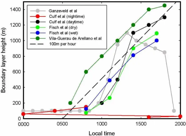
(MLH) in the early morning in the range 180–288 m h−1 and a maximum height of 1200 m at 13:00 Local Time (LT). They also reported residual layers persisting in the day and nightime that were not associated with any active vertical transport. Culf et al. (1997) highlighted the fact that a correctly parameterised boundary layer was impor-tant in their analysis of the CO2 concentrations over the Amazonian rain forest. They

5

used radiosondes and tethered balloons together with a gradient of potential temper-ature approach to diagnose the MLH. The rate of increase in the MLH was found to be approximately 175 m h−1between 10:00 LT and 14:00 LT. The average maximum in the MLH was 1300 m (±300 m,±1σ) and occurred at 17:00 LT. The important issue of

characterising the nocturnal boundary layer was also addressed and it was suggested

10

that the relative humidity profile, rather than the potential temperature profile, was the more appropriate parameterisation tool. This analysis indicated a nocturnal boundary layer height of the order 30 m at 20:00 LT, rising through the night to approximately 150 m at 08:00 LT. Therefore, there was an inferred collapse rate of the MLH between 17:00 LT and 20:00 LT of>400 m h−1. These results are summarised in Fig. 1. Param-15

eterisation of the boundary layer and the characteristics of the mixed layer height over a higher latitude forest environment has been analysed by Joffre et al. (2001).

Fisch et al. (2004) and Fisch and dos Santos (2008) have studied the influences of season and land usage on the Amazonian boundary layer. Radiosonde data and a potential temperature gradient analysis were again employed together with sodar data.

20

Figure 1 also shows these data. The approximate rates of increase in the mean MLH in the time intervals 08:00–11:00 LT, 11:00–14:00 LT and 14:00–17:00 LT were 64, 210 and 64 m h−1in the dry season and 122, 107 and 63 m h−1in the wet season respec-tively. The sodar data was shown to be influenced by residual layers. Vila-Guerau de Arellano et al. (2009) have studied the isoprene fluxes in the tropical rainforest

en-25

(5)

ACPD

10, 5021–5049, 2010

G. Pearson et al.

Title Page

Tables Figures

◭ ◮

Back Close

Full Screen / Esc

Ganzeveld et al. (2008) analysed nitrogen oxides, ozone and VOCs in the tropical boundary layer. They highlighted the issue that climate models had previously esti-mated too shallow a boundary layer over tropical forests primarily due to a misrepre-sentation of the surface energy balance. Their simulations suggested an increase in the MLH of 300 m (up to a typical maximum of 1400 m) if the soil moisture stress

func-5

tion was adjusted to a more representative value. It was also noted that when shallow cumulus clouds formed at altitudes of 1–3 km, the potential temperature gradient did not always indicate an explicit inversion height leading to an uncertainty in the effective MLH as derived from radiosondes. The results published for the MLH in the context of the simulated HCHO mixing ratio, show the diurnal variation portrayed in Fig. 1 with a

10

nightime MLH of the order 100 m and an increase up to approximately 1100 m at local noon. The rate of increase of the MLH between 10:00 LT and 12:00 LT was approx-imately 225 m h−1 and the collapse rate to the nocturnal state between 18:00 LT and 19:30 LT was approximately 500 m h−1.

Krejci et al. (2004) used radiosondes to study the Amazonian boundary layer in the

15

context of aerosol distributions. Their analysis of the MLH was based upon relatively sparse sampling but they observed heights of 800 m at 09:00 LT, increasing to 1170 m at 11:00 LT. The maximum rate of increase they observed was 360 m h−1but a value of half this was stated as being more typical. The MLH at local noon was determined to be in the region 1200–1500 m. In terms of their detailed aerosol results, it is interesting

20

to note that they reported a periodic strong gradient in the N120(number density of par-ticles>0.12 µm) particle fraction around 400 m, with the values below this level being

5–10 times higher than those aloft. In general their results show complicated and vari-able vertical profiles of the accumulation mode aerosol indicating that this alone would be an ambiguous tracer of mixed layer height. Amazonian aerosols distributions were

25

(6)

ACPD

10, 5021–5049, 2010

G. Pearson et al.

Title Page

Tables Figures

◭ ◮

Back Close

Full Screen / Esc

in the night. With a strong diurnal variation in the aerosol number density, care must be taken in interpreting backscatter profiles in the context of the dynamic processes in the near surface region.

3 Lidar observations of the boundary layer

Active optical remote sensing with pulsed lidar instrumentation o_ffers a unique view on

5

the atmosphere. Systems are available that rely on molecular, atomic or particulate scattering and numerous modes of operation with multiple data products are possible (Weitkamp, 2005). Remote sensing of the MLH with ground based lidar instrumenta-tion has concentrated on the use of characteristic features in the vertical distribuinstrumenta-tion of aerosols (Flamant et al. 1997; Menut et al., 1999; Dupont et al., 1999; Davis et

10

al., 2000; Matthias and Bosenberg, 2002; Hennemuth and Lammertt, 2006; Haij et al., 2007). Marsik et al. (1995) presented an inter-comparison of rawinsondes, a wind profiler (with Radio Acoustic Sounding System, RASS, for temperature profiling) and two lidars for determination of the MLH. Considerable variability was found between the various approaches. It was noted that the lidar backscatter data and analysis

con-15

sistently produced the lowest estimation of MLH. This was attributed to the fact that the aerosols that were acting as the tracer were not mixed up to the point where the rawin-sondes were indicating the threshold potential temperature gradient. It was suggested that the lidars were giving an effective mixing depth but it was also emphasised that the lidar approach could give erroneous results due to residual layers and clouds.

20

Grimsdell and Angevine (1998) reported results comparing radar wind profiler, ra-diosonde and ceilometer data in the context of determining the MLH and Steyn et al. (1999) extended the (sometimes subjective) prior approaches of a critical gradient or critical absolute backscatter to include a model of the entire aerosol backscatter profile. This was shown to be a more robust technique that was better able to accommodate

25

(7)

ACPD

10, 5021–5049, 2010

G. Pearson et al.

Title Page

Tables Figures

◭ ◮

Back Close

Full Screen / Esc

used a combination of two lidars (one of which was a pulsed Doppler instrument) and a radar wind profiler to study the MLH and the entrainment zone. While the lidar Doppler data was shown, it was not specifically used in the analysis. The wavelet approach utilised in their analysis was shown to be problematic when clouds and residual layers were present and, to avoid ambiguities, they excluded data outside the time interval

5

10:00–17:00 LT. Another issue that was alluded to, that is particularly relevant to trop-ical environments, was the interaction of the aerosol and humidity profiles due to the possible hydrophilic nature of the aerosol.

Davies et al. (2007) reported inter-comparions of pulsed Doppler lidar data with ra-diosondes and the outputs of several simulations. Again, although the lidar instrument

10

was Dopplerised, this data was not employed in the estimation of MLH. A subjective gradient of the backscatter profile approach was utilised. An important point was made here with respect to the MLH and the Lifting Condensation Level (LCL), as parame-terised in the Met O_ffice Unified Model (UM). In the parameterisation scheme of the UM, for the case of cumulus capped boundary layers, the MLH is set at the LCL.

15

The influence of humidity on the vertical aerosol backscatter distribution was further studied within the context of convection and depolarisation by Gibert et al. (2007). Relative Humidity (RH) was shown to be an important factor that influences the lidar signal since it modifies the size, shape, absorption and scattering of the aerosols. In addition, the possible hysteresis of particle size growth in a variable relative humidity

20

field may further complicate any interpretations with respect to mixing processes. Accordingly, they emphasise that aerosol backscatter coefficient alone cannot be directly interpreted as being a tracer for the MLH. These issues of humidity and MLH versus LCL are of particular relevance in tropical environments.

Recent field campaigns with pulsed Doppler lidar instruments have begun to show

25

(8)

ACPD

10, 5021–5049, 2010

G. Pearson et al.

Title Page

Tables Figures

◭ ◮

Back Close

Full Screen / Esc

the vertical transport directly, without the need to infer the dynamics from secondary measurements such as aerosol distributions or potential temperature gradients.

4 Description of instrument and deployment

The lidar deployed to Borneo was a pulsed Doppler instrument that had previously been used for studying the boundary layer in mid-latitude, European environments

5

(Pearson et al., 2009). It is a commercial device manufactured by Halo Photonics Ltd. The system relies on backscatter from aerosols and provides range gated Doppler and return power measurements. From these primary data products, wind profiles, turbulence parameters, backscatter coefficients and cloud base measurements can be derived. The spatial and temporal resolutions are variable but were fixed at values of

10

30 m and 2 s respectively for this deployment. The Doppler measurement precision is typically of the order 10 cm s−1 or less in the boundary layer (Pearson et al., 2009). The instrument was equipped with an all-sky scanner and was housed in a stand-alone enclosure. Full remote control including configuring the scan schedule, the data acquisition parameters and data off-load was achieved over the internet.

15

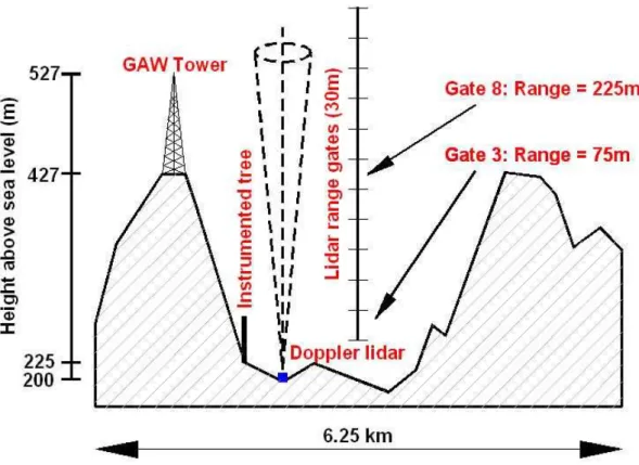
The instrument was located at the Nursery site (117.859◦E, 4.977◦N, El: 198 m) in the Danum valley region of Sabah, Borneo. The lidar site was in a valley, approx-imately 225 m below the base of the 100 m high Global Atmospheric Watch (GAW) tower (117.844◦E, 4.981◦N, El: 426 m) which was heavily instrumented with chemical and particulate sampling equipment for the duration of the experiment. The

topogra-20

phy of the 44 000 ha Danum valley region is hilly and consists of an undulating ground surface, with a relatively uniform virgin rain forest canopy, dissected by the Segama river and its tributaries. The highest point is Mount Danum (1093 m). The valleys are approximately 200 m deep. Figure 2 shows a cross-section of the local topography around the lidar site.

(9)

ACPD

10, 5021–5049, 2010

G. Pearson et al.

Title Page

Tables Figures

◭ ◮

Back Close

Full Screen / Esc

The scanner was configured to take wind profiles every 0.5 h and to stare vertically for the intervening periods. Each ray used in the wind profile consisted of the average of the distributed return signal from 60 000 consecutive laser pulses. The lidar oper-ated at a pulse rate of 20 kHz and therefore this was achieved using a 3 s stare time. The total time (including signal processing) taken to produce each wind profile was

5

approximately 4 min 50 s. For the vertical data, 40 000 pulses were averaged per ray and the update rate was approximately once every 13.5 s. There were therefore of the order 114 rays per vertical stare file. For both the stare and wind profile data, 200, 30 m range gates were recorded.

The data collection period spanned 3 April to 20 June 2008. The weather in the

Bor-10

neo region is relatively constant throughout the year. Average monthly temperatures are 25–26◦C and there are typically 4–6 h of sunshine per day. At night the valleys regularly experience low cloud that dissipates with the onset of significant insolation in the morning. The wet season is between November and February when the average monthly rainfall approximately doubles from 250 mm to 500 mm. This region is locally

15

referred to as the “Land below the Wind” because it is located below the typhoon belt. However, the name is doubly appropriate since the near surface winds are typically low.

5 Results and discussion

Apart from some intermissions due to power outages, a continuous data set was

ob-20

tained between 3 April and 19 June encompassing the OP3-I and OP3-II observation periods. A total of 1656 h of data were recorded, a testament to the autonomous ca-pacity of the instrument since it was unttended and operated remotely for this entire period. The overall aim of the data capture and subsequent analysis was to generate a statistically valid averaged data set for use in correctly parameterising the tropical

25

(10)

ACPD

10, 5021–5049, 2010

G. Pearson et al.

Title Page

Tables Figures

◭ ◮

Back Close

Full Screen / Esc

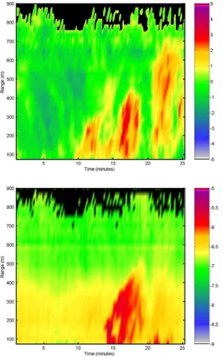
Figure 3 shows the typical temporal and spatial evolution of convection in the mid-morning period of the tropical day as observed at the Nursery site on 24 April 2008. The upper and lower panels show the vertical velocity and aerosol backscatter respectively versus time and height for a 25 min period commencing at 11:00 LT. Convective up-drafts can be readily seen in the upper panel and entrained aerosol being transported

5

therein is evident in the lower panel. The peak updraft velocity is approximately 2.5– 3 ms−1. Two features of the updrafts illustrated well here are that they do not always exhibit an enhanced aerosol content and they can be seen to extend to heights well above the region where the backscatter exhibits a strong negative gradient. The fact that the aerosol is not always entrained in the updraft is interesting in the context of

in-10

ferring the MLH from aerosol backscatter measurements. It has been noted previously that when different techniques are compared, values derived from lidar backscatter often show the lowest MLH values which is reasonable if this characteristic is preva-lent. The reduction in the backscatter at around 400 m is not easily explained since a number of other measurements are necessary in order to know the humidity field, the

15

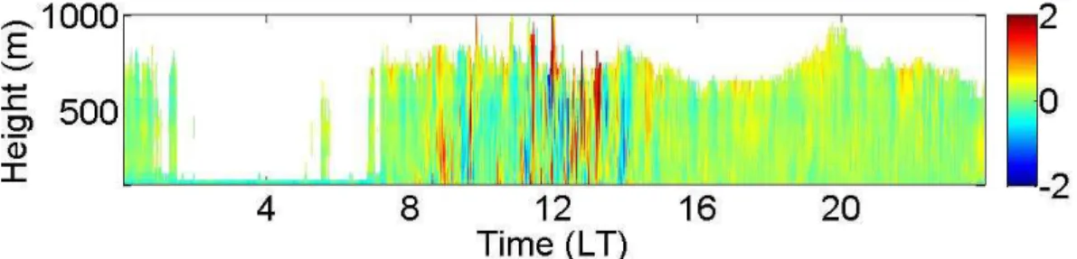
aerosol particle size distributions and the aerosol type. It is worth recalling the result of Krejci et al. (2004) where the same height was alluded to in the context of a change in the characteristics of the accumulation mode aerosol distribution. Figure 4 shows the typical daily development, extent and cessation of convection activity. The period of intense convective activity can be seen to exist between 09:00 LT and 15:00 LT.

20

The entire data record was analysed with a view to obtaining the statistics of the daily character of the boundary layer and cloud coverage. In this tropical environment, due to the consistent nature of the daily weather conditions, it was expected that the daily cycles of the boundary layer characteristics would show a high level of repeatability. In order to assess the stationarity of the data sets and consequently an appropriate

25

(11)

ACPD

10, 5021–5049, 2010

G. Pearson et al.

Title Page

Tables Figures

◭ ◮

Back Close

Full Screen / Esc

noise floor (wideband Signal to Noise Ratio (SNR)>−17 dB) and again with an SNR

band set to include the subset of data with SNRs in the range −17 dB to −5 dB. The first threshold includes all data (cloud and aerosol) and the second threshold was set so as to detect the return signal predominately from aerosols, excluding clouds. The return power data was converted to attenuated backscatter values based upon the

5

known calibration of the instrument. The vertically pointing Doppler data was analysed in terms of the standard deviation of the range-gated measurements per 25 minute period. All the data above the noise floor was included in this analysis. The aerosol distributions were computed by taking the difference between the “all data” and “cloud only” averages. It can be seen that there is a high degree of similarity between the

10

plots for the two successive weeks shown. This similarity was retained throughout the whole 10 week data set and stationarity testing indicated that averaging of the whole record was statistically valid. This would certainly not be the case for similar data sets over western Europe.

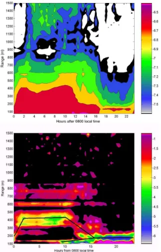
Figure 6 shows a contour plot of the averaged daily backscatter versus height

(eval-15

uated for the entire 10 week data collection period) as derived from the subset of data with SNR values in the range−5 dB to −17 dB. In the lowest 900 m, this sub-set of data corresponds predominately to returns from aerosols. Above this height, the plot shows the weak cloud returns from the aerosol – cloud interface at cloud base and the similarly weak returns from pulses that have undergone significant attenuation by

20

virtue of a round trip path within the cloud. The region of relatively high backscatter in-dicated by the red region shows a growth in height starting at around 07:30 LT, leading to a plateau region with an upper bound at approximately 400 m altitude. The rate of increase in the height of this region in the early morning was approximately 200 m h−1. There is a slight increase in the height of this region at around 18:00 LT and then a

25

(12)

ACPD

10, 5021–5049, 2010

G. Pearson et al.

Title Page

Tables Figures

◭ ◮

Back Close

Full Screen / Esc

positions of the maximum gradient, the feature conventionally used for determination of the MLH. The region of large negative gradient in the day-time aerosol signal is well highlighted as is a lower layer which grows through the evening. The transition between these and the humidity/aerosol interaction gives rise to ambiguities in the interpretation of these features in the context of mixed layer height.

5

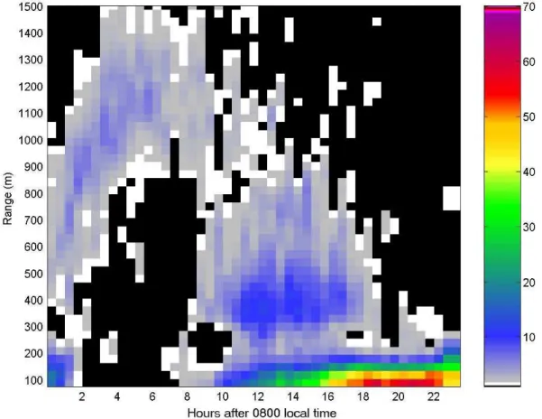
Figure 7 shows the averaged daily backscatter versus height (evaluated for the en-tire 10 week data collection period) as derived from the subset of data with SNR values

>−5 dB. The colour scale in this case indicates the occurrence, as a percentage, where

white corresponds to 1% and black is<1%. These data predominately show returns

from clouds. The void in the plot roughly bounded by the times 10:00 LT and 18:00 LT

10

and the heights 75 m and 700 m is nominally cloud free. The low level nocturnal cloud that consistently forms in the valley is readily seen between 20:00 LT and 08:00 LT. It can be seen that the frequency of occurrence of the nocturnal low-level cloud is of the order 60% though the period 02:00–06:00 LT. This observation is consistent with the visual observations from the GAW tower that indicated the valleys to be regularly in

15

cloud in the early morning. In the rest of the parameter space, it can be seen that the frequency of cloud coverage reaches values of around 10%. The zone of the plot exhibiting a slightly higher percentage value at a height of around 400 m, starting at 18:00 LT, corresponds to the analogous feature in the aerosol data of Fig. 6. The choice of the SNR threshold value used to split the aerosol/cloud returns clearly

in-20

fluences how this feature appears in these two figures and again highlights the issue of unambiguously interpreting the backscatter gradients. It seems reasonable that the aerosol feature is coupled to a humidity effect and reflects those occasions where the humidity was approaching that required for large-scale nucleation of cloud droplets.

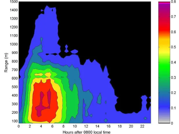
Figure 8 shows the average diurnal cycle in the standard deviation of the vertical

25

(13)

ACPD

10, 5021–5049, 2010

G. Pearson et al.

Title Page

Tables Figures

◭ ◮

Back Close

Full Screen / Esc

diurnal cycle in the vertical mixing without the ambiguities associated with interpreting aerosol backscatter levels. The zone comprising the green, yellow and red colours can be seen to exhibit a degree of correlation with the cloud free zone of Fig. 7 but shows different behaviour to that reflected in the gradient of the aerosol field. This is consistent with the model approach of Davies et al. (2007) where the MLH and the LCL

5

were matched for cumulus capped boundary layers. For the purposes of comparison, the 0.3 ms−1contour is replotted in Fig. 10.

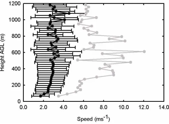
For the duration of the deployment, twice per hour, a wind profile was determined by conically scanning the beam over 12 individual inclined lines-of-sight. The mean, maximum and standard deviation of the wind speed versus height, as recorded at local

10

noon, for the duration of the deployment, are shown in Fig. 9. Shear can seen in the region near the ground, which is also below the valley rim. Above this, the average speed is approximately constant with height at around 3 ms−1. The typical values of the vertical velocity during active mixing are therefore similar to those of the horizontal flow, consistent with the phrase the “land below the wind”.

15

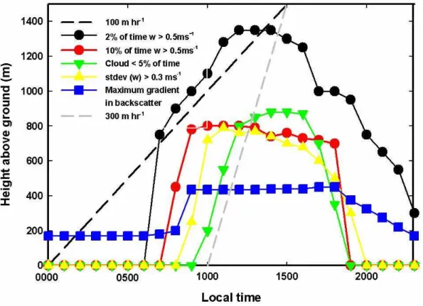
Figure 10 shows a review of the diurnal MLH variation as characterised by various analyses of the pulsed Doppler lidar data acquired during the 10 week deployment. The blue plot shows the profile in the maximum gradient of the backscatter. This metric is influenced by humidity, residual layers and is un-representative through the night. The green line represents the level indicated by the cloud base where we have used

20

an occurrence of 5% as the threshold. The red and black data are derived from the ver-tical velocity statistics and are based upon the regions where the verver-tical velocity was greater than 0.5 ms−1 2% (black) and 10% (red) of the time respectively. The yellow points are based upon the 0.3 ms−1contour of the averaged standard deviation in the vertical velocity. The two dashed lines show rates of 100 m h−1 and 350 m h−1. All the

25

(14)

ACPD

10, 5021–5049, 2010

G. Pearson et al.

Title Page

Tables Figures

◭ ◮

Back Close

Full Screen / Esc

and thresholded Doppler data (red plot, 10% of the time vertical velocity>0.5 ms−1).

The nocturnal MLH is not well characterised by the lidar since the minimum range of the data is 75 m and the valley is predominately cloud bound during this period. However, the lidar data does indicate that the there is negligible vertical motion in the nocturnal low cloud region implying that there is little vertical transport at night. This does not

5

preclude the possibility of nocturnal valley and drainage flows which may be active in the region below 75 m.

The fact that the lidar was located in the bottom of one of the many valleys in the region means that the data and particularly the nocturnal data are only applicable to this portion of the terrain. It would be expected that the ridges between the valleys

10

(i.e. where the GAW tower is located) will be influenced more by the horizontal flow and will be subject to di_fferent nocturnal conditions since they are above the low lying cloud.

6 Conclusions

Within the frame work of the OP3 experiment, a pulsed Doppler lidar system has been

15

deployed to the rain forest of north east Borneo in order to characterise the tropical boundary layer. The transport of chemical species and particulates from the surface and canopy layers of the forest into the lower levels of the atmosphere is governed by the dynamics of boundary layer. The lidar can remotely measure these characteristics providing a data set which allows the surface based point sampling measurements to

20

be further analysed within the wider context of the regional atmosphere.

The range gated backscatter and vertical velocity data from the lidar have been anal-ysed with a view to compiling a climatology that can be used in interpreting and extrap-olating the surface and tower based point measurements. Repeatable daily cycles in the aerosol backscatter, vertical velocity and cloud base profiles have been shown to

25

(15)

ACPD

10, 5021–5049, 2010

G. Pearson et al.

Title Page

Tables Figures

◭ ◮

Back Close

Full Screen / Esc

The vertical gradient of the aerosol backscatter, cloud base, vertical velocity dis-tributions and the standard deviation of vertical velocity approaches to characterising the MLH have been compared for the same 70 day long data collection period in the nominal dry season. The different techniques have been summarised and the results should enable a refinement of the way in which the tropical boundary layer is

param-5

eterised. There are important differences in the rates of increase and decay in the MLH and in the measured characteristics at nighttime for the different methods of data analysis. Interpretation of the aerosol backscatter data is shown to be complicated by the influences of clouds and humidity. The Doppler velocity measurements reported here are a direct measurement of the mixing process and it is suggested that this is the

10

most appropriate methodology to use in analysing the dispersion of canopy sourced species into the lower atmosphere. It is also proposed that secondary indicators used for the determination of MLH such as radiosondes, backscatter lidar profiles and wind profilers will, on occasions, not indicate the actual active mixing height but either the height to which mixing would occur if the process was initiated or the mixing height that

15

was appropriate in the recent past. Sporadic daytime solar occultation by clouds, shad-owing within valleys, sunrise, sunset and aerosol/humidity interactions are examples of situations when this issue might be important.

These experimentally determined spatial and temporal characteristics in the aver-aged diurnal vertical velocity, cloud and aerosol statistics in the tropical boundary layer

20

are currently being used to aid interpretation of the OP3 data set and it is envisaged that these data will find future applications in the parameterisation of global climate models.

Acknowledgements. We would like to thank the staffat the Nursery site, the Danum valley field station and all those members of the OP3 team you offered their help and support in both the 25

(16)

ACPD

10, 5021–5049, 2010

G. Pearson et al.

Title Page

Tables Figures

◭ ◮

Back Close

Full Screen / Esc

References

Cohn, S. A. and Angevine, W. M.: Boundary layer height and entrainment zone thickness measured by lidars and wind-profiling radars, J. Appl. Meteorol., 39, 1233–1247, 2000. Culf, A. D., Fisch, G., Malhi, Y., and Nobre, C. C.: The influence of the atmospheric boundary

layer on carbon dioxide concentrations over a tropical forest, Agr. Forest Meteorol., 85, 149– 5

158, 1997.

Davis, K. J., Gamage, N., Hagelberg, C. R., Kiemble, C., Lenschow, D. H., and Sullivan, P. P.: An objective method for deriving atmospheric structure from airborne lidar observations, J. Atmos. Ocean. Tech., 17, 1455–1468, 2000.

Davies, F., Middleton, R. R., and Bozier, K. E.: Urban air pollution modelling and measurements 10

of boundary layer height, Atmos. Environ., 41, 4040–4049, 2007.

de Haij, M. J., Klein Baltink, H., and Wauben, W. M. F.: Continuous mixing layer height de-termination using the LD-40 ceilometer: a feasibility study, Scientific Report WR 2007-01, Koninklijk Nederlands Meteorologisch Instituut (KNMI), De Bilt, 2007.

Dupont, E., Menut, L., Carissim, B., Pelon, J., and Flamant, P.: Comparison between the 15

atmospheric boundary layer in Paris and its rural suburbs during the ECLAP experiment, Atmos. Environ., 33, 979–994, 1999.

Eerdekens, G., Ganzeveld, L., Vil `a-Guerau de Arellano, J., Kl ¨upfel, T., Sinha, V., Yassaa, N., Williams, J., Harder, H., Kubistin, D., Martinez, M., and Lelieveld, J.: Flux estimates of iso-prene, methanol and acetone from airborne PTR-MS measurements over the tropical rain-20

forest during the GABRIEL 2005 campaign, Atmos. Chem. Phys., 9, 4207–4227, 2009, http://www.atmos-chem-phys.net/9/4207/2009/.

Elbert, W., Taylor, P. E., Andreae, M. O., and P ¨oschl, U.: Contribution of fungi to primary biogenic aerosols in the atmosphere: wet and dry discharged spores, carbohydrates, and inorganic ions, Atmos. Chem. Phys., 7, 4569–4588, 2007,

25

http://www.atmos-chem-phys.net/7/4569/2007/.

Fisch, G. and dos Santos, L. A. R.: Estimates of the height of the boundary layer using Sodar and rawinsoundings in Amazonia, 14th Symposium for the advancement of boundary layer remote sensing, IOP Conference series: Earth and Environmental Science, 1, 2008. Fisch, G., Tota, J., Machado, L. A. T., Silva Dias, M. A. F., da Lyra, R. F., Nobre, C. A., Dolman, 30

(17)

ACPD

10, 5021–5049, 2010

G. Pearson et al.

Title Page

Tables Figures

◭ ◮

Back Close

Full Screen / Esc

Interactive Discussion Flamant, C., Pelon, J., Flamant, P. H., and Durand, P.: Lidar determination of the entainment

zone thickness at the top of the unstable marine atmospheric boundary layer, Bound.-Lay. Meteorol., 83, 247–284, 1997.

Frehlich, R., Millier, Y., Jensen, M. L., and Balsley, B.: Measurements of boundary layer profiles in an urban environment, J. Appl. Meteorol. Clim., 45, 821–837, 2006.

5

Ganzeveld, L., Eerdekens, G., Feig, G., Fischer, H., Harder, H., K ¨onigstedt, R., Kubistin, D., Martinez, M., Meixner, F. X., Scheeren, H. A., Sinha, V., Taraborrelli, D., Williams, J., Vil `a-Guerau de Arellano, J., and Lelieveld, J.: Surface and boundary layer exchanges of volatile organic compounds, nitrogen oxides and ozone during the GABRIEL campaign, At-mos. Chem. Phys., 8, 6223–6243, 2008,

10

Garrett, A. J.: A parameter study of interactions between convective clouds, the convective boundary layer and a forested surface, Mon. Weather Rev., 110, 1041–1059, 1982.

Gibert, F., Cuesta, J., Yano, J.-I., Arnault, N., and Flamant, P. H.: On the correlation between convective plume updrafts and downdrafts, lidar reflectivity and depolarization ratio, Bound.-15

Lay. Meteorol., 125, 553–573, 2007.

Grimsdell, A. W. and Angevine, W. M.: Convective boundary layer height measurement with wind profilers and comparison to cloud base, J. Atmos. Ocean. Tech., 15, 1331–1338, 1998. Hennemuth, B. and Lammert, A.: Determination of the atmospheric boundary layer height from

radiosonde and Lidar backscatter, Bound.-Lay. Meteorol., 120, 181–200, 2006. 20

Hewitt, C. N., Lee, J. D., MacKenzie, A. R., Barkley, M. P., Carslaw, N., Carver, G. D., Chappell, N. A., Coe, H., Collier, C., Commane, R., Davies, F., Davison, B., DiCarlo, P., Di Marco, C. F., Dorsey, J. R., Edwards, P. M., Evans, M. J., Fowler, D., Furneaux, K. L., Gallagher, M., Guenther, A., Heard, D. E., Helfter, C., Hopkins, J., Ingham, T., Irwin, M., Jones, C., Karunaharan, A., Langford, B., Lewis, A. C., Lim, S. F., MacDonald, S. M., Mahajan, A. 25

S., Malpass, S., McFiggans, G., Mills, G., Misztal, P., Moller, S., Monks, P. S., Nemitz, E., Nicolas-Perea, V., Oetjen, H., Oram, D. E., Palmer, P. I., Phillips, G. J., Pike, R., Plane, J. M. C., Pugh, T., Pyle, J. A., Reeves, C. E., Robinson, N. H., Stewart, D., Stone, D., Whalley, L. K., and Yin, X.: Overview: oxidant and particle photochemical processes above a south-east Asian tropical rainforest (the OP3 project): introduction, rationale, location characteristics 30

(18)

ACPD

10, 5021–5049, 2010

G. Pearson et al.

Title Page

Tables Figures

◭ ◮

Back Close

Full Screen / Esc

Interactive Discussion Hogan, R. J., Grant, A. L. M., Illingworth, A. J., Pearson, G. N., and O’Connor, E. J.: Vertical

velocity variance and skewness in clear and cloud-topped boundary layers as revealed by Doppler lidar, Q. J. Roy. Meteor. Soc., 135, 635–643, 2009.

Joffre, S. M., Kangas, M., Heikinheimo, M., and Kitaigorodskii, S. A.: Variability of the stable and unstable atmospheric boundary-layer height and its scales over a Boreal forest, Bound.-Lay. 5

Meteorol., 99, 429–450, 2001.

Krejci, R., Str ¨om, J., de Reus, M., Williams, J., Fischer, H., Andreae, M. O., and Hansson, H.-C.: Spatial and temporal distribution of atmospheric aerosols in the lowermost troposphere over the Amazonian tropical rainforest, Atmos. Chem. Phys., 5, 1527–1543, 2005,

http://www.atmos-chem-phys.net/5/1527/2005/. 10

Lelieveld, J., Butler, T. M., Crowley, J. N., Dillon, T. J., Fischer, H., Ganzeveld, L., Harder, M., Lawrence, M. G., Martinez, M., Taraborrelli, D., and Williams, J.: Atmospheric oxidation capacity sustained by a tropical forest, Nature, 452, 737–740, 2008.

Marsik, F. J., Fischer, K. W., McDonald, T. D., and Samson, P. J.: Comparison of methods for estimating mixing height used during the 1992 Atlanta filed intensive, J. Appl. Meteorol., 34, 15

1802–1814, 1995.

Martin, C. L., Fitzjarrald, D., Garstang, M., Greco, S., Oliveira, P. A., and Browell, E.: Structure and growth of the mixing layer over the Amazonian rain forest, J. Geophys. Res., 93, 1361– 1375, 1988.

Matthias, V. and B ¨osenberg, J.: Aerosol climatology for the planetary boundary layer derived 20

from regular lidar measurements, Atmos. Res., 63, 221–245, 2002.

Menut, L., Flamant, C., Pelon, J. and Flamant, P. H.: Urban boundary-layer height determination from lidar measurements over the Paris area, Appl. Optics, 38, 945–954, 1999.

Pearson, G. N., Davies, F., and Collier, C.: An analysis of the performance of the UFAM pulsed Doppler lidar for observing the boundary layer, J. Atmos. Ocean. Tech., 26, 240–250, 2009. 25

Pike, R. C., Lee, J. D., Young, P. J., Moller, S., Carver, G. D., Yang, X., Misztal, P., Langford, B., Stewart, D., Reeves, C. E., Hewitt, C. N., and Pyle, J. A.: Can a global model chemical mechanism reproduce NO, NO₂, and O₃measurements above a tropical rainforest?, Atmos. Chem. Phys. Discuss., 9, 27611–27648, 2009,

(19)

ACPD

10, 5021–5049, 2010

G. Pearson et al.

Title Page

Tables Figures

◭ ◮

Back Close

Full Screen / Esc

Interactive Discussion Pugh, T. A. M., MacKenzie, A. R., Hewitt, C. N., Langford, B., Edwards, P. M., Furneaux, K.

L., Heard, D. E., Hopkins, J. R., Jones, C. E., Karunaharan, A., Lee, J., Mills, G., Misztal, P., Moller, S., Monks, P. S., and Whalley, L. K.: Simulating atmospheric composition over a South-East Asian tropical rainforest: performance of a chemistry box model, Atmos. Chem. Phys., 10, 279–298, 2010,

5

Steyn, D. G., Baldi, M., and Hoff, R. M.: The detection of mixed layer depth and entrainment zone thickness from lidar backscatter profiles, J. Atmos. Ocean. Tech., 16, 953–959, 1999. Tucker, S. C., Brewer, W. A., Banta, R. M., Senff, C. J., Sandberg, S. P., Law, D. C., Weickmann,

A., and Hardesty, R. M.: Doppler lidar estimation of mixing height using turbulence, shear, 10

and aerosol profiles, J. Atmos. Ocean. Tech., 26, 673–688, 2009.

Vil `a-Guerau de Arellano, J., van den Dries, K., and Pino, D.: On inferring isoprene emission surface flux from atmospheric boundary layer concentration measurements, Atmos. Chem. Phys., 9, 3629–3640, 2009,

http://www.atmos-chem-phys.net/9/3629/2009/. 15

Warneke, C., Holzinger, R., Hansel, A., Jordan, A., Lindinger, W., P ¨oschl, U., Williams, J., Hoor, P., Fischer, H., Crutzen, P. J., Scheeren, H. A., and Lelieveld, J.: Isoprene and Its oxidation products methyl vinyl ketone, methacrolein, and isoprene related peroxides measured online over the tropical rain forest of Surinam in March 1998, J. Atmos. Chem., 38, 167–185, 2001. Weitkamp, C.: Lidar: Range resolved optical remote sensing of the atmosphere, Springer 20

(20)

ACPD

10, 5021–5049, 2010

G. Pearson et al.

Title Page

Tables Figures

◭ ◮

Back Close

Full Screen / Esc

Interactive Discussion Fig. 1. A summary of previous experimental and theoretical results for the MLH above the

(21)

ACPD

10, 5021–5049, 2010

G. Pearson et al.

Title Page

Tables Figures

◭ ◮

Back Close

Full Screen / Esc

Interactive Discussion Fig. 2. A schematic cross section of the terrain around the lidar site from the NW (left|) to the

(22)

ACPD

10, 5021–5049, 2010

G. Pearson et al.

Title Page

Tables Figures

◭ ◮

Back Close

Full Screen / Esc

Interactive Discussion Fig. 3. An example of a 25 min observation of the vertical velocity (upper panel) and aerosol backscatter coefficient

(23)

ACPD

10, 5021–5049, 2010

G. Pearson et al.

Title Page

Tables Figures

◭ ◮

Back Close

Full Screen / Esc

Interactive Discussion Fig. 4. An example of the daily vertical velocity field as recorded on 15 April 2008. The colour

(24)

ACPD

10, 5021–5049, 2010

G. Pearson et al.

Title Page

Tables Figures

◭ ◮

Back Close

Full Screen / Esc

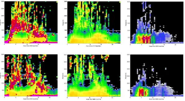
Interactive Discussion Fig. 5. These plots show diurnal cycles, as averaged over a week, for the first 2 weeks of the

deployment. The top row corresponds to week 1, starting 3 April 2008, and the second row to week 2. The three columns, from the left, are backscatter value (all data with SNR>−17 dB),

backscatter value (data for SNR values between−5 dB and−17 dB) and standard deviation of the vertical velocity evaluated from all the data with an SNR>−17 dB. The backscatter colour

(25)