https://doi.org/10.5194/amt-10-3463-2017 © Author(s) 2017. This work is distributed under the Creative Commons Attribution 3.0 License.
Perdigão 2015: methodology for atmospheric multi-Doppler
lidar experiments
Nikola Vasiljevi´c1, José M. L. M. Palma2, Nikolas Angelou1, José Carlos Matos3, Robert Menke1, Guillaume Lea1, Jakob Mann1, Michael Courtney1, Luis Frölen Ribeiro3,4, and Vitor M. M. G. C. Gomes2
1DTU Wind Energy, Technical University of Denmark, Frederiksborgvej 399, Building 118-VEA, 4000 Roskilde, Denmark 2Faculty of Engineering of the University of Porto, Rua Dr. Roberto Frias, 4200-465 Porto, Portugal
3Institute of Science and Innovation in Mechanical and Industrial Engineering, Rua Dr. Roberto Frias,
4200-465 Porto, Portugal
4Polytechnic Institute of Bragança, Campus de Santa Apolónia, 5300-253 Bragança, Portugal Correspondence to:Nikola Vasiljevi´c ([email protected])
Received: 20 January 2017 – Discussion started: 15 February 2017
Revised: 2 August 2017 – Accepted: 4 August 2017 – Published: 21 September 2017
Abstract.The long-range and short-range WindScanner sys-tems (LRWS and SRWS), multi-Doppler lidar instruments, when combined together can map the turbulent flow around a wind turbine and at the same time measure mean flow condi-tions over an entire region such as a wind farm. As the Wind-Scanner technology is novel, performing field campaigns with the WindScanner systems requires a methodology that will maximize the benefits of conducting WindScanner-based experiments. Such a methodology, made up of 10 steps, is presented and discussed through its application in a pilot experiment that took place in a complex and forested site in Portugal, where for the first time the two WindScanner systems operated simultaneously. Overall, this resulted in a detailed site selection criteria, a well-thought-out experiment layout, novel flow mapping methods and high-quality flow observations, all of which are presented in this paper.
1 Introduction
In wind energy research, field experiments are important for wind resource evaluation but also to establish, validate and improve theories and wind flow models. If experiments are well planned, designed, executed and reported, the field datasets have a long lifetime and are a firm basis for the ad-vancement of our knowledge on atmospheric flows.
A large number of field experiments addressing flows over hills (see Taylor et al., 1987) were carried out between 1979
and 1986. These field experiments provided the experimen-tal validation of the models of the wind industry resource assessment (Jackson and Hunt, 1975; Mortensen et al., 2004; Walmsley et al., 1986). Among the field experiments of the past, the Askervein hill experiment (Taylor and Teunissen, 1987; Walmsley and Taylor, 1996) is an example of a field campaign dataset that has been in use for more than 30 years. The increased computational power and developments in both numerical techniques and implementation of the flow physics have enabled the use of computational fluid dynam-ics (CFD) and mesoscale models at a larger scale, which calls for validation with new field experiments. The need for new and higher quality field datasets, recognized in various wind-energy-related forums (e.g., EWEA, 2005, 2008; Shaw et al., 2009; van Kuik et al., 2016), is driven by the increasing size of the modern wind turbines often located in complex oro-graphies.
measurements, single lidars can retrieve accurate wind vec-tor information if the flow is horizontally homogeneous (see Courtney et al., 2008; Peña Diaz et al., 2009). In complex terrain, the flow rarely satisfies this assumption, which leads to erroneous retrievals of the wind vector by single lidars (Bingöl et al., 2009).
Employing at least two lidars and intersecting their beams at a point of interest is required to directly measure two com-ponents of the wind at that point, while to fully characterize the wind vector at least three laser beams should intersect at a given point. By moving the beam intersection over an area or volume of interest, the flow can be mapped and resolved in two or all three dimensions. Dual-Doppler setups consist-ing of two scannconsist-ing lidars have been used in several large atmospheric studies (e.g., McCarthy et al., 1982; Newsom et al., 2005; Collier et al., 2005; Grubiši´c et al., 2008), while their application in wind-energy-related studies is rather re-cent (e.g., Iungo et al., 2013; Newsom et al., 2015). Triple-lidars were primarily used to demonstrate the capability of accurately retrieving the wind vector in a single point (Mann et al., 2009) or in multiple points distributed along a single vertical axis (see virtual masts in Fuertes et al., 2014; New-man et al., 2016; Lundquist et al., 2017).
As discussed in Vasiljevi´c et al. (2016a), lidars in the previously mentioned studies were individually configured, run and monitored; thus, there was no central computer that would ensure their synchronicity. Also, commercially avail-able lidars were used in the majority of these studies, and the configuration flexibility and available auxiliary information of such devices is usually limited (e.g., no accurate timing of scans and only simple scanning methods are available).
Efforts put into the WindScanner.dk project have resulted in two specific and highly configurable multi-Doppler lidar instruments, known as the long-range and short-range Wind-Scanner systems (LRWS and SRWS; Mikkelsen, 2014), specifically designed to address the aforementioned needs of wind energy research for new measurements. These instru-ments unlocked the potentials not only to measure the wind field at a single point located within the rotor-swept area but also to map entire wind fields within the volume occupied by modern wind turbines and wind farms. As the WindScanner systems are a novel and extremely flexible wind measure-ment technology, there is an increased chance of misconduct-ing experiments and not producmisconduct-ing the best possible results. In order to maximize the benefits of using the WindScanner technology, there is a need to establish a methodology for WindScanner-based atmospheric experiments.
In this paper, we propose such a methodology. The methodology will be discussed through its application to a pilot experiment, Perdigão 2015, that took place in a com-plex and forested site in Portugal, where the two WindScan-ner systems were operated simultaneously for the first time. In addition, the methodology and operation of the Wind-Scanner systems, this paper also presents a review of the two WindScanner systems, novel scanning methods,
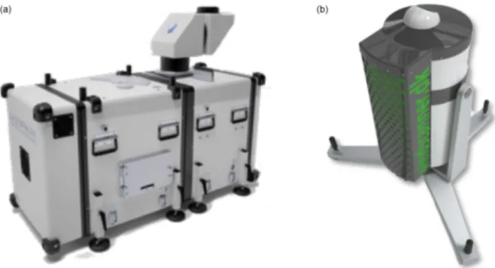
obser-Figure 1.DTU Wind Energy scanning lidars. Long-range Wind-Scanner(a); short-range WindScanner(b).
vational highlights of multi-lidar measurements of a single turbine wake and inflow conditions in complex terrain, multi-lidar measurements of wind resources along a ridge and ob-servations of valley flows. It should be pointed out that the data analysis or discussions of particular flow situations are not the purpose of the present paper and are included as a result and as an illustration of the presented methodology.
The paper is organized as follows: Sect. 2 describes the WindScanner systems, Sects. 3 and 4 present the methodol-ogy and a detailed description of how it was applied, the re-sults of the methodology demonstration and future work are presented in Sect. 5, while Sect. 6 provides the concluding remarks.
2 WindScanner systems
A WindScanner system consists of two or more spatially separated scanning lidars (long- or short-range WindScan-ners, Fig. 1) that are coordinated or controlled by a master computer. The first generations of the long-range WindScan-ner (LRWS) and short-range WindScanWindScan-ner (SRWS) orig-inate from commercially available vertical profiling lidars Windcube 200 and ZephIR respectively. Under the Wind-Scanner.dk project, DTU Wind Energy, with the expert sup-port from specialized industrial partners, developed scanner heads, converting the profiling lidars into the scanning li-dars that make up the LRWS and SRWS. In addition to the hardware developments, DTU Wind Energy developed spe-cific software solutions for both WindScanner systems (e.g., Vasiljevi´c et al., 2016a).
control-ling them using a MACRO (Motion and Control Ring Opti-cal) digital interface (see Delta Tau, 2017).
SRWSs provide high-frequency measurements (up to 400 Hz) of the flow while probing the atmosphere with a rela-tively small probe length. This allows resolving small length scales (down to a few cm) and short time scales (down to 2.5 ms) of the flow. As SRWSs are based on the continu-ous wave (CW) lidar technology there are several limitations. Since the LOS speed at a given point is resolved by focus-ing the laser beam, the probe length increases with range. This limits the maximum range of a SRWS to about 150 m. Furthermore, since the beam can only be focused at a single point in time, radial velocity from one single range can be re-solved. However, a high measurement rate compensates for this limitation in ranging. Based on these characteristics the short-range WindScanner system is ideal for mapping of tur-bulent flow features around a single wind turbine rotor (e.g., Immas et al., 2015) or around a small scale orographic fea-ture (e.g., Lange et al., 2016).
LRWSs have a larger probe length (minimum 25 m) and lower measurement frequency (10 Hz at best, typically 1 Hz) than SRWSs. Since LRWSs are based on the pulsed technol-ogy their probe length is constant with range. Furthermore, LRWSs can simultaneously retrieve radial velocity from a number of ranges along the laser light propagation path. This number is limited by the computational power of the lidar. This particular characteristic of ranging compensates for a lower measurement frequency since at any given measure-ment rate LRWS can provide a “snapshot” of the atmosphere up to several kilometers along a single LOS. The maximum range of LRWSs is about 8 km, which has been typically ob-served in offshore conditions (Floors et al., 2016). Due to its characteristics, the long-range WindScanner system is pri-marily intended for measurements of mean flow fields within a large area of the atmosphere (e.g., Berg et al., 2015).
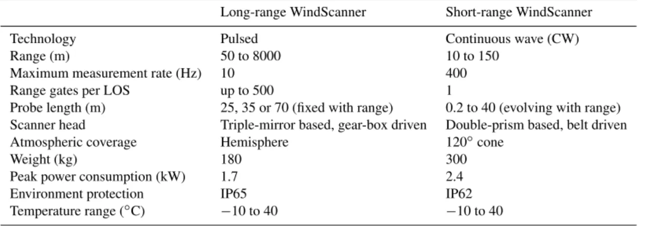
A summary of the characteristics of the two types of Wind-Scanners is given in Table 1. A more detailed description of the long-range WindScanner system is provided in Vasiljevi´c (2014b) and Vasiljevi´c et al. (2016a), while Mikkelsen et al. (2011) and Sjöholm et al. (2014) include additional details on the short-range WindScanner system.
Based on the characteristics of the two multi-lidar instru-ments, the long- and short-range WindScanner systems are complementary to each other. Combining these two systems into a hybrid system unlocks a possibility of simultaneously observing mean flow features over a large region and turbu-lent characteristics and fine flow structures within a prese-lected area (not larger than a rotor-swept area) of this same region. At the current state of the lidar technology, we cannot have all these capabilities within one single system.
The campaign Perdigão 2015, described in the present paper, was the first attempt to simultaneously operate both long- and short-range WindScanner systems with an aim of combining them into a hybrid WindScanner system and ac-quiring both mean and turbulent flow features of the site.
3 Methodology
The methodology for WindScanner-based experiments con-sists of 10 steps: (1) definition of scientific objectives, (2) site selection, (3) site characterization, (4) experiment layout de-sign, (5) scanning modes dede-sign, (6) infrastructure plan-ning, (7) deployment and calibration, (8) execution and data collection, (9) decommissioning and post-calibration, and (10) data archiving and dissemination.
Defining scientific objectives is related to outlining scien-tific questions of interest that can be addressed with Wind-Scanner observations. According to the scientific objectives, the site selection is made and followed by a detailed site char-acterization (e.g., wind conditions, terrain). Sometimes the order is reversed – a known site can stimulate a scientific question.
In the following steps, the experiment layout is made and physical infrastructure is planned (e.g., power, network, ac-cess roads). Afterwards, given the now-established logisti-cal constraints, the scanning modes to be implemented dur-ing the campaigns are designed. Once the physical installa-tion commences, the deployment and calibrainstalla-tion procedural steps are applied (e.g., leveling and orientation of WindScan-ner, assessment of pointing accuracy). Following the start of the campaign, the execution and data collection procedural steps are put in action (e.g., experiment monitoring and infor-mation logging). The decommissioning and post-calibration procedural steps are applied at the end of the campaign. In the last procedural step, all the data regarding the campaign are collected together with the acquired datasets and uploaded to an online information system, making them available for end users.
The aforementioned steps will be demonstrated in the con-tent of the Perdigão-2015 experiment in the following sec-tion.
4 Perdigão-2015 implementation of methodology There were multiple reasons in favor of the Perdigão-2015 experiment: there was the need to test both the equipment and our human resources in a demanding field experiment. The question was whether the new scientific equipment, which is expensive, fragile and sensitive, and has been developed and tested previously in a laboratory environment or in short-duration field campaigns was robust enough to withstand re-alistic conditions; for instance, high temperatures and remote locations with no power or network grid. The equipment, transported by road between Roskilde (Denmark) and Serra do Perdigão (Portugal) and remained in the mountains with-out surveillance for long periods.
fi-Table 1.Characteristics overview of the WindScanners.
Long-range WindScanner Short-range WindScanner
Technology Pulsed Continuous wave (CW)
Range (m) 50 to 8000 10 to 150
Maximum measurement rate (Hz) 10 400
Range gates per LOS up to 500 1
Probe length (m) 25, 35 or 70 (fixed with range) 0.2 to 40 (evolving with range) Scanner head Triple-mirror based, gear-box driven Double-prism based, belt driven
Atmospheric coverage Hemisphere 120◦cone
Weight (kg) 180 300
Peak power consumption (kW) 1.7 2.4
Environment protection IP65 IP62
Temperature range (◦C)
−10 to 40 −10 to 40
nanced. Among the project deliverables, the methodology for WindScanner-based field experiments (which we report in the present paper) was developed based on the previous extensive work done under the WindScanner.dk project (see Vasiljevi´c et al., 2016a; Sjöholm et al., 2014). The method-ology was brought in to be tested and was further improved in a campaign held in Kassel (Germany) during the summer of 2014 (Pauscher et al., 2016; Vasiljevi´c et al., 2016a).
Perdigão 2015 was a last demonstration campaign within the WindScanner.eu project that served as the preparation for the larger experiment conducted within the NEWA project (New European Wind Atlas, Mann et al., 2017) at the same site in 2017. Perdigão 2015 took place during the summer of 2015, from 4 May until 29 June.
4.1 Step 1: definition of scientific objectives
In addition, the WindScanner.eu project, Perdigão 2015 was funded by the NEWA, Unified Turbine Testing (UniTTe), and Wind Farm Layout Optimization in Complex Terrain (Far-mOpt) projects. The latter three projects have specific re-search goals that assisted in defining scientific objectives for Perdigão 2015.
The NEWA project aims to improve wind resource model-ing for different site conditions. Areas with steep ridges and forested terrain are of particular interests since the current engineering (linear) flow models are unable to correctly pre-dict the behavior of the flow over the sites with these features (Palma et al., 2008). The UniTTe project is focused on im-proving international standards for characterizing the wind power and load measurements of wind turbines on various sites (e.g., flat and complex terrain) by substituting mast-based measurements with measurements derived by nacelle-mounted lidars measuring close to the turbine rotor. To fulfill this project’s ambition, it is necessary to investigate how the incoming flow is modified by a wind turbine. The objective of the FarmOpt project is to develop numerical tools for wind farm layout optimization in complex terrain. Here it is nec-essary to adequately model the wind turbine wake in
com-plex terrain. To address the aforementioned scientific ques-tions, all three projects, NEWA, UniTTe and FarmOpt, call for wind field measurements in complex terrain, preferably measurements of both mean and turbulent characteristics of the flow field, where UniTTe and FarmOpt specifically re-quire that those measurements are done in the vicinity of a wind turbine rotor. Perdigão 2015 offered the opportunity to acquire such measurements.
For Perdigão 2015, we selected several flow aspects to in-vestigate and addressed them with WindScanner measure-ments. To assist the NEWA project, we chose to measure wind resources along a ridge, occurrences of flow separa-tions on lee sides of hills (i.e., recirculation zone) and valley flows. For the FarmOpt project, we intended to characterize a single wind turbine wake in horizontal and vertical planes. Specifically, we aimed to provide measurements for studying the wind speed deficit up to five diameters downstream of the wind turbine, the wake position in a vertical plane close to the wind turbine, and the wake geometry in a horizontal plane with center at the wind turbine hub. Similarly, for the UniTTe project, the inflow conditions were intended to be characterized in the same planes. The objective was to derive datasets for a detailed investigation of the wind turbine in-duction zone in complex terrain. The ultimate objective was to create a dataset that could be used in the appraisal and de-velopment of computational models for wind resource, wind turbine design and wind farm layout optimization in complex terrain.
4.2 Step 2: site selection
clear boundary conditions. Providing that this requirement is almost never met in nature, realistically, the surround-ing terrain’s complexity should be significantly lower than the selected site’s complexity. A quasi two-dimensional, or a long-ridge, hill is a logical choice, and, to assure a two-dimensional flow, dominant winds should be perpendicular to the ridge. Land cover, particularly forests, would add to the flow complexity and is considered desirable since many wind farms are installed near or within forested regions. Ac-cording to these criteria, the Perdigão site was selected. The presence of a wind turbine at the site provided the opportu-nity for wake and inflow measurements.
It should be noted that the site selection is typically made considering specific criteria or the site itself triggers ideas for experiments. In the case of the Perdigão site, it was both. In 2009, the site visit initiated the idea for a double-hill exper-iment. In 2014, due to the presence of the wind turbine, the site became an eligible location for a measurement campaign addressing the wake and inflow conditions of wind turbines in complex terrain.
4.3 Step 3: site characterization
Perdigão (Fig. 2) is formed by two parallel ridges, with southeast–northwest orientation and a distance circa 1.4 km, that measure about 4 km lengthwise and are 500–550 m above sea level (a.s.l.) at their summits. The valley-to-peak height is about 200 to 250 m and the hills are steep, with an inclination of approximately 35 %. A double ridge in com-parison to a single-ridge site provides a list of additional ad-vantages because the lee-side flow is also the flow impinging on the second ridge. Furthermore, the lee side of the first hill and the upwind side of the second hill make up the valley flow. The terrain coverage is irregular, made of no or low-height vegetation and patches of eucalyptus and pine trees. Southwest and northeast from the ridges the terrain flattens somewhat, providing an environment that to a first approx-imation can provide definable inflow conditions. An Ener-con E-82 2 MW operating wind turbine is located on the south ridge (Fig. 2).
Perdigão is an ideal site in terms of the orography and main road access, but with a difficult access to the ridges. The access to ridges is mostly through poorly maintained, steep and narrow unpaved roads, which creates difficulties for the equipment installation. During late springs and sum-mers, the daytime temperatures are frequently above 30◦C,
which imposes a challenge for field work. Overall, Perdigão provided a unique and demanding environment.
The site orography and canopy were mapped in March 2015 during a helicopter laser mapping mission. The area of 20 km2was scanned, showing a density of about 40 points per square meter. Orthophotos with a resolution of 5 and 20 cm of the same area were acquired along with the derived point cloud. Wind measurements from the site were available from a 40 m meteorological tower (INEGI, 2005)
Table 2.Wind characteristics (January 2002–December 2004).
Height (a.g.l.; m) 10 20 40
Measured days 1096 1096 1096
Wind speed
Mean (m s−1) 5.0 5.0 5.8
Max (m s−1) 24.8 23.8 22.8
Turbulence intensity
V >5 m s−1(%) 10.0 8.9 9.1
14< V <15 m s−1(%) 8.5 7.7 8.6
Weibull parameters
A(m s−1) 5.6 6.3 6.5
k 1.8 2.0 2.0
from January 2002 to December 2004 (3 years, Table 2), with an 88 % availability at location 33997 Easting, 3529 Northing and an altitude of 489 m a.s.l. at three heights (10, 20 and 40 m) above ground level (a.g.l.). The predominant winds were from the northeast and west–southwest direc-tions (Fig. 3), i.e., perpendicular to the ridges, with a mean and maximum wind speed of around 6 and 20 m s−1
respec-tively (Table 2 and Fig. 3). These directions are also those with highest average velocity (Fig. 3) and lowest levels of turbulent intensity.
4.4 Step 4: experiment layout design
Computer simulations (Gomes, 2011) based on the VENTOS® Castro et al. (2003) code of the flow over Perdigão were of importance while designing the experi-ment layout. VENTOS®is a dedicated CFD code for solv-ing atmospheric boundary layer (ABL) flows over complex terrain, based on the elliptical RANS equations and thek-ε
parame-South ridge
Valley
North ridge
Turbine
Valley
North ridge
(a)
(b)
Figure 2.Perdigão site in September 2014 (see Vasiljevi´c, 2014a). Views from the north ridge(a)and south ridge(b).
� �� �
��
�
��
�
�� �� �� ��� ��� ���
� �� �
��
�
��
�
�� �� �� �� �� ��
� �� �
��
�
��
�
�� �� ��� �� ��� ��� ���� ��� (
a) ( )b ( )c
Figure 3.Wind regime at met mast station for 3-year period at 40 m a.g.l.:(a)wind direction (%);(b)wind speed (m s−1);(c)turbulence intensity (%).
ters were calibrated to yield wind speeds of 5–6 m s−1at the
south ridge under southwest winds, with a surface character-istic roughnessz0set to 0.03 and friction velocityu∗set to
0.23 m s−1. The simulations of the flow from the northeast
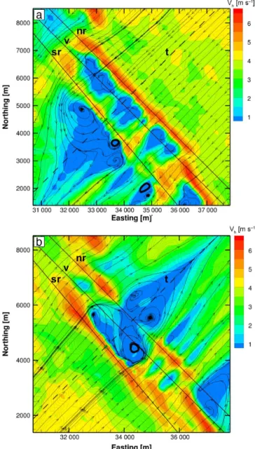
and southwest predict a high complexity of the flow (Fig. 4) and large recirculation zone enclosed in the valley (Fig. 5).
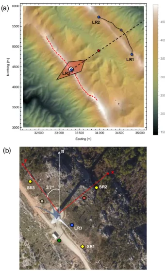
The two WindScanner systems comprised a total of six scanning lidars: three LRWSs, named Koshava (LR1), Sterenn (LR2) and Whittle (LR3); and three SRWSs, named R2D1 (SR1), R2D2 (SR2) and R2D3 (SR3). The lidar lo-cations were selected with the aim of sampling the flow field along the south ridge and within the transect perpendicular to the ridges that goes through the wind turbine (Fig. 6 and Ta-ble 3), while taking into account intersecting angles between
laser beams and elevation angles at which the laser beams will be directed.
We define the intersecting angle as the smallest angle be-tween the projections of two intersecting laser beams in a horizontal plane. The intersecting angle can take any value between 0 and 90◦
. When selecting lidar locations we intend to have an intersecting angle of at least 30◦
with respect to the prevailing wind direction. Based on a simple accuracy model (see Vasiljevi´c and Courtney, 2017) the intersecting angle of 30◦
results in an accuracy of about 0.25 m s−1 for
the retrieved horizontal wind speed. In order to accurately retrieve the vertical wind speed, the elevation angles should be as steep as possible, preferably 90◦as indicated in
Figure 4.Simulated wind flow on a surface 80 m a.g.l.:(a) north-east winds; (b) southwest winds. Positions expressed in datum ETRS89/PTM06 (m) (EUREF, 2016). Three thick diagonal lines denoted as sr,vand nr represent the south ridge, valley and north ridge lines. The dashed line denotedtrepresents the transect of in-terest.
uses a norm approach described in Simley et al. (2016) to as-sess the suitability of the multi-Doppler setup, the elevation angles larger than 45◦ provide means to accurately acquire
the vertical component.
The previously acquired point cloud and orthophotos as-sisted in choosing the most accessible locations for the Wind-Scanners’ installation with respect to the previously estab-lished criteria. LR3 was located on the south ridge next to the wind turbine, and LR1 and LR2 were located on the north ridge (Fig. 6a). The distance from LR3 to LR1 and from LR3 to LR2 was about 1.5 km, while the distance between LR1
Figure 5.Simulated wind flow in a vertical plane indicated by the dashed line in Fig. 4:(a)northeast winds;(b)southwest winds. The coordinate system origin corresponds to the wind turbine base.
and LR2 was about 1.2 km. The three SRWSs were located on the south ridge close to the wind turbine (Fig. 6b): SR1 and SR3 close to the access road, 52 m southeast and 45 m northwest of the wind turbine respectively; and SR2 43 m northeast of the wind turbine, down the slope of the south ridge (Table 3 and Fig. 6b).
4.5 Step 5: infrastructure planning
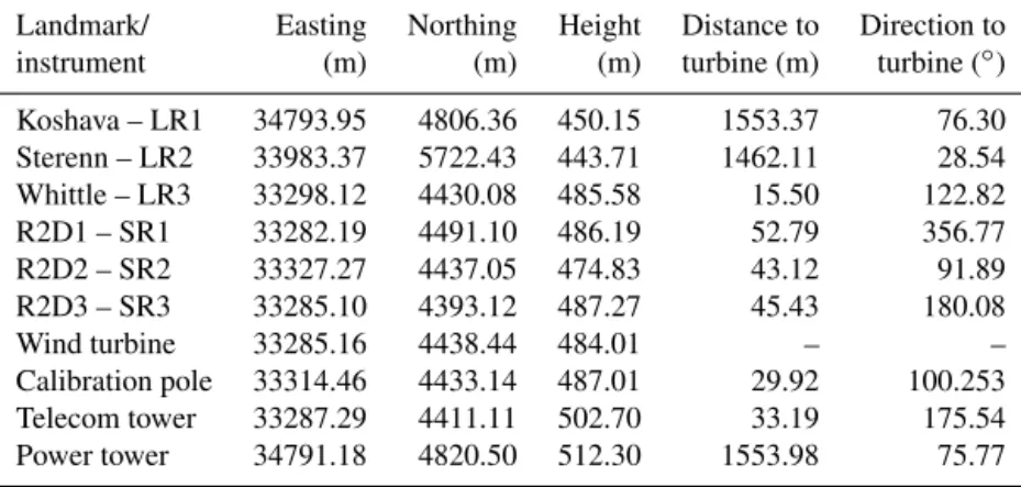
de-Table 3.Position of instruments and landmarks given in datum ETR89/PTM06 (m).
Landmark/ Easting Northing Height Distance to Direction to
instrument (m) (m) (m) turbine (m) turbine (◦)
Koshava – LR1 34793.95 4806.36 450.15 1553.37 76.30
Sterenn – LR2 33983.37 5722.43 443.71 1462.11 28.54
Whittle – LR3 33298.12 4430.08 485.58 15.50 122.82
R2D1 – SR1 33282.19 4491.10 486.19 52.79 356.77
R2D2 – SR2 33327.27 4437.05 474.83 43.12 91.89
R2D3 – SR3 33285.10 4393.12 487.27 45.43 180.08
Wind turbine 33285.16 4438.44 484.01 – –
Calibration pole 33314.46 4433.14 487.01 29.92 100.253
Telecom tower 33287.29 4411.11 502.70 33.19 175.54
Power tower 34791.18 4820.50 512.30 1553.98 75.77
ployment. It should be noted that without the local support achieving the aforementioned experiment layout would be almost impossible (see Vasiljevi´c, 2015a, for more details). 4.6 Step 6: deployment and calibration procedures After all scanning lidars were positioned, oriented and lev-eled at the designated locations (see Vasiljevi´c, 2015b), their absolute positions were acquired using a multi-station (combination of total station and GPS) in conjunction with DGPS–RTK correction data (accuracy about 1 cm). The cor-rection data were provided by the Geographic Institute of the Portuguese Army. Additionally, the absolute position of sev-eral landmarks (e.g., wind turbine, telecom tower) were ac-quired and used for the WindScanner’ calibration.
For assessing the pointing accuracy of LRWSs, selected landmarks were mapped with the LRWS laser beams us-ing the CNR (carrier-to-noise) mapper (Vasiljevi´c, 2014b, p. 157). The power line tower on the north ridge was mapped with LR3, whereas the telecom tower next to the wind turbine was mapped with LR1 and LR2. The comparison of the ref-erenced and mapped positions indicated a pointing accuracy of 0.05◦
in azimuth and elevation for all three LRWSs. From the CNR maps, we were able to determine the backlash level of 0.025◦
, which is consistent with results from previous de-ployments (see Vasiljevi´c et al., 2016a). The sensing range accuracy was assessed using the same landmarks. The laser beams were steered to hit the landmarks, and we assessed the range gate positions (i.e., distances along LOS) at which the intensity of the backscattered light (CNR) was maximum since these positions correspond to the distances between the landmarks and LRWSs. We found sensing range offsets of 8, 10 and 3 m for LR1, LR2 and LR3 respectively, which were corrected for during the design of the scanning methods.
Since the DC component in the SRWS Doppler spectra is notched out, non-moving hard targets cannot be used to assess their pointing and sensing range accuracy. Instead of non-moving targets, for the SRWSs we employed a 12 m cal-ibration pole with two motor-driven balls on the top made
of low-density polyether (Fig. 7a). The rotating balls were scanned simultaneously from the three SRWSs by mapping three separate 2 m×2 m vertical planes, oriented perpendic-ular to the pointing direction of each instrument. In Fig. 7b, the result of such a scan is presented, where only the sig-nals from the two rotating balls are highlighted. When the mapped positions of the balls were compared with the ref-erence positions, we found a similar pointing accuracy level in the SRWSs to that of the LRWSs. The rotating balls were also used to assess the sensing range accuracy. The three laser beams were steered to meet the center of the top rotating ball, and the focus points were moved along the laser beam prop-agation paths. The results of this test, Fig. 8, depict the in-tensity of the backscattered signal of each of the SRWSs ver-sus the distance of focusing and the theoretical distribution of the intensity based on the assumption that the intensity of a focused laser beam follows a Lorentzian distribution. It is assumed that the maximum intensity appears at the distance where the moving target is located in regards to a SRWS. It has been found that the calculated and measured distances corresponded to each other to within a few centimeters. 4.7 Step 7: scanning modes design
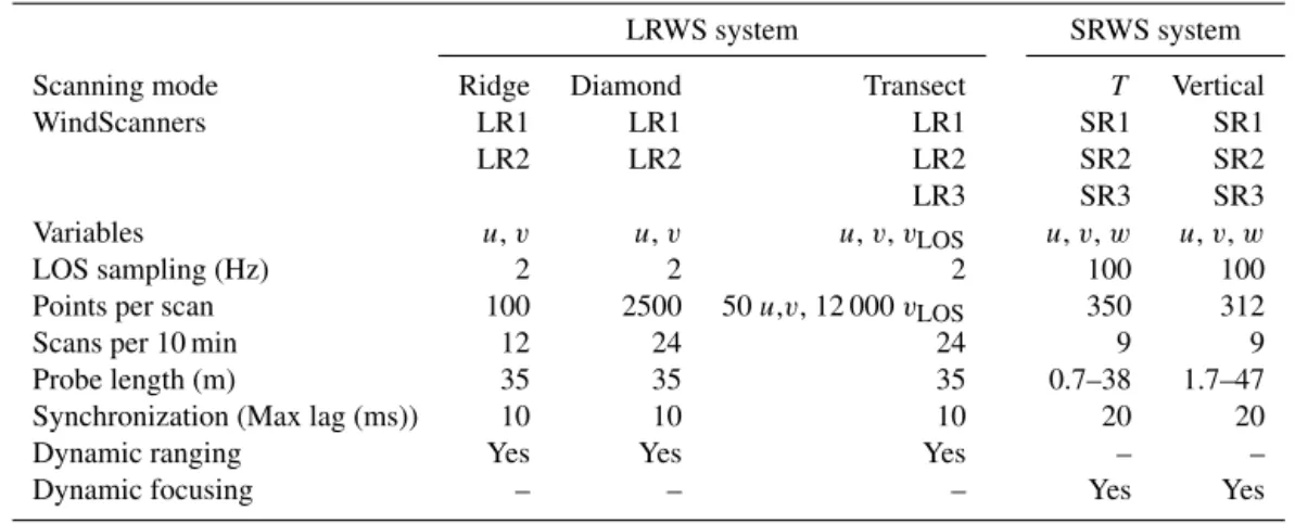
Five scanning modes, Table 4, were designed to investigate the flow details around the wind turbine and in the valley: ridge, diamond and transect scans, in the case of the LRWSs; andT and vertical plane scans, in the case of the SRWSs.
The ridge scan was designed to address the flow above the south ridge (Table 4 and Fig. 6). The two LRWSs, LR1 and LR2, were configured to intersect their laser beams and to move the beam intersection along a curved line 2 km long, 80 m above the crest (i.e., the wind turbine hub height), fol-lowing the terrain profile (see Vasiljevi´c, 2016c). The line was designed using the point cloud information. The mean elevation angle at which both laser beams were directed was 4.11◦
. Throughout the scan, on average the intersecting angle between the two laser beams was 42.21◦
32 500 33 000 33 500 34 000 34 500 35 000 3000
3500 4000 4500 5000 5500 6000
Easting [m]
Nort
hing
[m
]
150 200 250 300 350 400 450
R2D1 R2D2
x y
37o N ( a)
b
LR1 LR2
LR3
LR3 SR2
SR1 SR3
( )
Figure 6.Perdigão site:(a)overall view (blue circles, long-range WindScanner units; white circle, wind turbine; pink quadrilateral, diamond scan; dashed black line, transect scan; red circle, virtual mast scan; solid black lines, power cables; red dashed line, ridge scan);(b)top view around the wind turbine (yellow circles, short-range WindScanner units; blue circle, long-short-range WindScanner unit LR3; grey circle, control center; red circle, calibration pole; green circle, telecom tower and substation).
To investigate the inflow and wake conditions of the wind turbine at a large scale, LR1 and LR2 were configured to guide the laser beams within a 4.7◦
vertically inclined quadri-lateral with the center at the turbine hub and dimensions of 500 m×750 m. The quadrilateral lies on an inclined horizon-tal plane defined by LR1, LR2 and hub position. The wind turbine hub represented the middle point of a 1 km long diag-onal of the quadrilateral. Along this diagdiag-onal, LR1 and LR2 synchronously intersect laser beams and move the beam in-tersection resolving instantaneous horizontal wind speed and wind direction (true dual-Doppler) at 50 points – thus every 20 m (see Vasiljevi´c, 2016a). Since the beams were guided within the same plane, this allowed the retrieval of horizon-tal wind speed and wind direction (unsynchronized) in an additional 2450 measurement points (Table 4 and Fig. 6). In
1.25 1. 0.75 0.5 0.25 0. 0.25 0.5 0.75 1. 1.25 0.5
0.25 0. 0.25 0.5 0.75 1. 1.25 1.5 1.75 2.
y m
z
m
10 8 6 4 2 0 2 4 6 8 10
vr ms1
a
b
Figure 7.Calibration of the SRWS:(a)actual setup (1 – telecom tower, 2 – calibration pole with two motor-driven balls and 3 – SRWS’s scanner head);(b)radial wind speeds induced from the rotation of the two rotating balls as measured by SR1 (the perimeter of the two balls is depicted with orange circles).
R2D1 R2D2 R2D3
0 20 40 60 80 100
0.0 0.2 0.4 0.6 0.8 1.0
d@mD
N
or
m
al
ized
integr
ated
spectr
um
@
-D
Figure 8. Integrated spectrum versus focus distances for SR1 (R2D1, black line), SR2 (R2D2, green line) and SR3 (R2D3, red line).
obtain data for studying the wind speed deficit up to five di-ameters downstream of the wind turbine, the wake position, and wake geometry in a horizontal plane with the center at the wind turbine hub, as well as the inflow conditions up to five diameters upstream of the wind turbine. The average in-tersecting angle between the two laser beams during the dia-mond scan was 49.37◦
, while the average elevation angle at which the beams were directed was 4.33◦
.
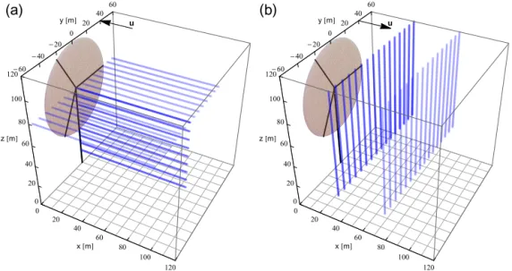
In addition to the large-scale flow observations, two scan-ning modes for the short-range WindScanner system (Table 4 and Fig. 9) were configured to provide insights on the inflow and wake at the turbine scale. The T-scan was used to mea-sure the turbine inflow conditions. Two different versions of this mode were used, differing in the dimensions of the scan-ning area. Both of them consisted of one vertical and one horizontal plane, which were perpendicular to each other and perpendicular to the south ridge line. In Fig. 9a, we can see the first version in the Cartesian coordinate system, with the origin in the wind turbine base rotated 37◦
clockwise from north. The area covered with the first scan mode version was from −56 to 56 m along the y axis, from 0 to 80 m along thex axis and from 14 to 78 m along thezaxis. Within the enclosed area, 15 horizontal and 9 vertical line scans were performed. The second version covered an area from−64 to 64 m along theyaxis, from−10 m to 100 m along thexaxis and from 14 to 78 m along thezaxis, encompassing 17 hori-zontal and 9 vertical line scans. On average, the intersecting angles between the SR1 and SR2, SR1 and SR3, and SR2 and SR3 laser beams were 44.26, 55.78 and 49.64◦
respec-tively. The average elevation angle at which the beams were directed was 50.92◦
.
To address the wake conditions with the short-range Wind-Scanner system, the vertical scan mode consisting of vertical lines was employed (Fig. 9b). Also, two different versions of the scanning mode were used. Both of them focused on
scan-ning in vertical lines placed in a plane parallel to the wind turbine’s rotor. The scanning plane was confined in they–z
plane, between−48 and 48 m alongy, and between 30 and 128 m alongz. In the first version of the scanning pattern, the vertically scanned lines were located in a vertical plane one rotor diameter (80 m) away. In the second version, one more plane with the same dimensions was added half a rotor diameter away in the downwind direction. On average, the intersecting angles between the SR1 and SR2, SR1 and SR3, and SR2 and SR3 laser beams were 28.77, 59.96 and 49.21◦
respectively. The average elevation angle at which the beams were directed was 49.91◦
.
While executing the second version of the T and verti-cal scan modes, we observed a lag (loss of synchronization) between SR3 and the other two SRWSs (SR2 and SR1), which operated in sync. The lag linearly increased over the time with a constant rate of 16.67 and 5000 µs s−1for theT
and vertical scan modes respectively. The observed lag was caused by the safety limits of the scanner head controller, which did not allow higher scanning speeds than the maxi-mum permitted speed for a safe operation. As a result, SR3 was lagging behind SR2 and SR1. The reset of the scanning modes zeroed the lag, which then once again increased over time as described. The reset took place each time when we switched from one scanning mode to another. However, this was not done in a systematic way since the scanning mode switching took place when the wind direction changed from the northeast to southwest. Therefore, the values of the max-imum lag for the short-range WindScanner system in Table 4 are only given for the first version of theT and vertical scan modes since during their execution the SRWSs were in sync. The transect scan was employed to investigate the flow field within a vertical plane perpendicular to the ridges en-tailing the wind turbine (Table 4, Figures 6 and 10). The three LRWSs were configured to perform intersecting and syn-chronized range–height indicator (RHI) scans. The RHI scan of LR3 coincided with the vertical plane (Figure 10), whereas other two RHI scans sliced through this plane along a 500 m vertical line position in the valley (see the vertical dashed line in Fig. 10). The radial wind field measured by LR3 pro-vided the possibility to assess the recirculation zone on lee sides of either ridge in the case of southwest and northeast winds, traces of the wind turbine wake and the flow in the valley (see Vasiljevi´c, 2016d). The intersection of the three RHI scans represented a 500 m virtual mast. The intersecting angle during the scan between the LR1 and LR2 laser beams was 84.10◦, while this angle between the LR2 and LR3 laser
beams and between the LR1 and LR3 was equal to 54.77 and 41.12◦
respectively. The elevation angle at which the beams were directed was in a range from about−12 to 23◦
u
0 20
40 60
80 100
120 x m
60 40
20 0
20 40
60
y m
0 20 40 60 80 100 120
z m
u
0 20
40 60
80 100
120 x m
60 40
20 0
20 40
60
y m
0 20 40 60 80 100 120
z m
( a) ( )b
Figure 9.Scanning patterns of short-range WindScanners:(a)T-scan;(b)vertical planes.
500 0 500 1000 1500 2000 2500
200 400 600 800 1000 1200 1400
Range m
Height
m
H
e
ig
h
t
a
.s
.l
.
[m
]
1400
1200
1000
800
600
400
200
-500 0 500 1000 1500 2000 2500
Range [m]
Figure 10.Transect scan: red lines indicate LOS measurements acquired by LR3, the vertical dashed line shows the position of the virtual mast, and the inclined horizontal dashed line indicates the position of the diamond scan plane.
The long-range WindScanner system’s scans were run in a batch mode, where each strategy was executed over a 10 min period. The sequence of the ridge, diamond and transect scan was executed over a 30 min period and then repeated. Be-cause only LR1 and LR2 were needed to execute the ridge and diamond scans, LR3 continued to perform the transect strategy throughout the entire campaign.
The Portuguese Institute for Sea and Atmosphere (IPMA) provided a daily forecast for the Perdigão site using a non-hydrostatic numerical weather prediction model of a limited area (AROME, the numerical prediction model of Meteo-France) for variables such as temperature, relative humid-ity, rain, wind direction and velocity at 10 m and 80 m a.g.l. The wind direction was used to decide the scanning mode of the short-range WindScanner system: the vertical mode if the wind was coming from the southwest direction (wake scanning) or the T-scan mode in the case of northeast wind (inflow scanning).
4.8 Step 8: execution and data collection
Table 4.Scanning modes.
LRWS system SRWS system
Scanning mode Ridge Diamond Transect T Vertical
WindScanners LR1 LR1 LR1 SR1 SR1
LR2 LR2 LR2 SR2 SR2
LR3 SR3 SR3
Variables u,v u,v u,v,vLOS u,v,w u,v,w
LOS sampling (Hz) 2 2 2 100 100
Points per scan 100 2500 50u,v, 12 000vLOS 350 312
Scans per 10 min 12 24 24 9 9
Probe length (m) 35 35 35 0.7–38 1.7–47
Synchronization (Max lag (ms)) 10 10 10 20 20
Dynamic ranging Yes Yes Yes – –
Dynamic focusing – – – Yes Yes
However, this was the first time the long- and short-range WindScanner systems were used simultaneously, and only a few periods of simultaneous measurements were collected, because of the following reasons. Despite the rapid installa-tion of the WindScanner systems, the off-grid power solu-tion for the long-range WindScanner system was deployed roughly 10 days after the short-range WindScanner system started collecting data. An issue with the control unit of one of the LRWSs forced us to reject the measurements during 23–25 May (see the blog post for these dates). The cool-ing systems of long- and short-range WindScanners could not cope with the high temperature around midday (≥40◦
C) and we had to pause the measurements for a couple of hours every day. We discussed this issue more in Vasiljevi´c et al. (2016a), where we suggested possible solutions. The short-range WindScanner system had a technical issue with the MACRO ring which halted the observations during June. 4.9 Step 9: decommissioning and post-calibration
procedures
At the end of the measurement period the pointing and sens-ing range accuracy were reassessed with the LRWSs only. We found that the new positions of the landmarks matched the previously mapped position within 0.05◦
in azimuth and elevation for all three LRWSs. The backlash levels remained the same – 0.025◦
. The new set of sensed distances showed no difference compared to the previously acquired set. Due to technical issues of the SRWSs, the post-calibration pro-cedure was not performed for this system. After the post-calibration procedure the WindScanners were uninstalled, and all traces of their presence removed from the sites. 4.10 Step 10: data dissemination and availability The short-range WindScanner system was operational from 8 May until 3 June. During this period, 110 h (665 runs with a duration of 10 min each) of data were acquired. A total of 407 runs were made with the T-scan mode, addressing
in-flow conditions, whereas the remaining 258 were made by employing the vertical planes mode, addressing wake condi-tions. The long-range WindScanner system was operational from 19 May until 26 June. Overall, the long-range Wind-Scanner system acquired 528 h of data, from which about 180 h of data were recorded with each scanning strategy. A special case is the transect scan, where in addition to the 180 h of concurring data acquired with all three LRWS there is also the additional 360 h of data collected only by LR3. There are 6 h of simultaneous measurements of the inflow conditions with both WindScanner systems.
Also, for the entire measurement period (May–June) the owner of the wind turbine (Generg) provided 10 min means of the wind turbine SCADA (supervisory control and data acquisition) data.
The acquired datasets of radial velocities were entirely processed and data artifacts removed. The LRWS dataset was filtered on the CNR values of each individual measurement point (CNR>−27 dB). In addition to the filtering, a multi-range gate analysis was applied to remove remaining spuri-ous data points where, using multi-peak detection in the CNR values for each LOS, data points contaminated with hard tar-gets were removed. Also, by detecting discrete jumps in the radial speed values along each LOS, errors in the spectral estimation were rejected from the datasets. Details about the multi-range gate analysis will be presented in a separate pub-lication.
Table 5.Data availability expressed in hours.
LRWS system
Scanning mode Ridge Diamond Transect
Data before filtering on sampling 187 185 181 Data after filtering on sampling 77 94 116
Northeasterly winds 7.5 10 15
Southwesterly winds 19 16 12
the data were spatially averaged after being grouped in cubic grid cells both of 4×4×4 m and 8×8×8 m dimensions. To treat the synchronization issues that appeared in the sec-ond versions of the T-scan and vertical plan patterns, the data acquired using those pattern versions were additionally time averaged in 10 min periods.
Where possible, the processed radial velocities were com-bined to calculate two (diamond, ridge and transect scanning methods) or all three components of the wind vector (T and vertical scanning method). Details about the retrieval tech-niques are given in Appendix A. Afterwards, the wind vec-tor and radial fields were averaged over a 10 min period and plotted. The resulting figures were saved as PNG files, which were available for users to visually browse the dataset. To indicate the amount of high-quality data collected with the long-range WindScanner system, we applied a simple fil-ter on sampling constraints affil-ter processing all data, which consisted of selecting only those 10 min runs where there was at least 50 % of the maximum number of scan iterations and at least 50 % of the maximum number of measurement points. The results are given in Table 5 only for the long-range WindScanner system. Currently, for the SRWS, each 10 min period is being manually evaluated in order to deter-mine whether the wake or induction zone are captured with measurements. This is the reason why Table 5 does not in-clude information on the SRWS data.
Both raw and highly processed datasets have been up-loaded to a MySQL database and are currently available for the participants of the projects that funded the experiment. We intend to release the entire dataset for public use during the second half of 2017 through the e-WindLidar web plat-form (http://e-windlidar.windenergy.dtu.dk). At present, the data are being analyzed by the research groups directly in-volved in Perdigão 2015 and have been presented in appro-priate forums. Examples of those presentations and publica-tions are, for instance, found in Mann et al. (2016) for the details of the experiment; in Rodrigues et al. (2016), who fo-cused on the flow in the valley and over the two ridges; in Hansen et al. (2016), who focused on the wind turbine wake; and in Meyer Forsting et al. (2016), who focused on the in-flow conditions.
5 Discussion
5.1 Observational results
Figures 11 to 15 intend to illustrate the performance of the scanning modes and also be a sample of the flow phenomena observed during the course of the field campaign.
The ridge scan, 2 km along the south ridge, shows no turn-ing of the wind for the northeast winds (Fig. 11a). Thus, for this wind direction we observed a two-dimensional flow. On the other hand, for southwest winds there is a slight turning of the wind (the difference between the wind direction at the edges of the transect is roughly 15◦
, Fig. 11b). The maximum wind speed along the transect is not seen at the wind turbine location regardless of the dominant wind direction (Fig. 11). The initial data analysis of the wake measurements indi-cates a clear diurnal dependence of the wake characteristics (see Hansen et al., 2016), which may be related to the stratifi-cation. Due to the lack of temperature and heat flux measure-ments, we established an empirical relation between the pe-riod of a day and atmospheric stability. A well-formed, nar-row and long wake was pulled down the slope during late nights until early mornings when we expected stable condi-tions and reduced mixing (Figs. 12a and 13a). On the other hand, during the rest of the day under more unstable con-ditions and increased mixing, the wake was wider, shorter and lifted up (Figs. 12b and 13b). The inflow and wake of the turbine during 1 full day is well represented in Vasiljevi´c (2016b).
The objective of the transect scans (Fig. 14) was the map-ping of the flow over the ridges and in the valley. For the dominant wind directions of the northeast and southwest (Fig. 14a and b), the recirculation zones on the lee sides (south side of the north ridge and north side of the south ridge) of the hills can be seen, as suggested by the compu-tational results in Fig. 5. Although they share a common fea-ture, these two figures correspond to 2 different days (7 and 10 of June) and two different times (03:29 and 13:43 UTC) – night and day at a time of low and high temperature. The ve-locity field at 03:29 UTC, Fig. 14a, displays a pattern, a two-layer atmosphere of maximum wind speed at around 500 and 750 m, and a constant wind speed between 500 and 650 m. Figure 14c, at around the same time in the night, displays a stratified atmosphere with a well-defined internal wave, orig-inating in the south ridge, of a length equal to the distance between ridges (see 24 h animation, Vasiljevi´c, 2016e). This phenomenon and the conditions under which it can persist, which is a subject in Rodrigues et al. (2016), will be studied further.
pe-1000 500 0 500 1000 5.5 6.0 6.5 7.0 7.5 8.0 8.5 9.0
Southeast Range m Northwest
Vh m s – 1 40 50 60 70 80 Wi n d d ir e cti o n ˚
32 500 33 000 33 500 34 000
3500 4000 4500 5000 5500 Easting m N o rth in g m
1000 500 0 500 1000
5.0 5.5 6.0 6.5 7.0 7.5 8.0
Southeast Range m Northwest
215 220 225 230 235 240 Wi n d d ir e cti o n ˚
32 500 33 000 33 500 34 000
3500 4000 4500 5000 5500 Easting m N o rth in g m ( a) b Vh m s – 1 ( )
Figure 11.Wind vectors, wind speed and direction (10 min averaged) 80 m a.g.l. along the south ridge for wind dominant directions acquired using the ridge scan performed by the long-range WindScanner system:(a)northeast (measurements taken on 7 June 2015 from 03:30 to 03:40 UTC);(b)southwest (measurements taken on 21 June 2015 from 21:42 to 21:52 UTC). Black line, horizontal wind speed; red line, wind direction; dashed red line, ridge scan; grey circle (left) and rectangle (right) are areas where measurements are erroneous due to the presence of the wind turbine.
riod the wind direction was approximately 45◦
; thus, the ro-tor plane was not completely aligned with the vertical plane scan (53◦), while the mean horizontal wind speed was about
4.5 m s−1 at the hub height. The comparison of the
long-and short-range WindScanner system horizontal wind speed measurements at horizontal lines closest to the two scanned plane intersections shows a generally good agreement (the averaged mean difference is about 0.2 m s−1). We should not
expect the exact match between these measurements since the way in which the flow was probed at the coinciding points with two WindScanner systems differs. Throughout the dia-mond scan the laser beams of the long-range WindScanner system were steered within a horizontal plane, whereas the laser beams of the shot-range WindScanner system during the vertical plane scan were directed with steep elevation an-gles (the averaged elevation angle was about 50◦
). In addi-tion, the difference in the positioning of the probes with re-spect to the measurement points, the probe lengths of the two WindScanner systems are also different (see Table 4). What effects the dimension and position of the intersecting probes have on the retrieved wind speed information will be studied in future publications.
5.2 Improving the methodology
In this paper, we presented the methodology for conducting field studies with multi-Doppler lidars. This was a prelimi-nary attempt at outlining and defining systematic steps that can lead to the acquisition of high-quality datasets from field studies. Despite being developed for multi-Doppler lidar ex-periments, the methodology can be used for any field cam-paign. The majority of the presented steps are relevant for all field experiments (e.g., defining scientific question, plan-ning infrastructure), while some are WindScanner specific (e.g., scanning mode design). In this paper, we presented a sequential execution of the steps. However, some steps can and should run in parallel (e.g., data archiving and dissem-ination with execution and data collection) and some steps can be merged together (e.g., experiment layout design and infrastructure planning).
simula-a
b
Figure 12.The wake in a horizontal plane observed with the dia-mond scan (10 min averaged) performed by the long-range Wind-Scanner system for different atmospheric conditions: (a) stable conditions (measurements taken on 10 June 2015 from 22:20 to 22:30 UTC); (b) unstable conditions (measurements taken on 11 June 2015 from 16:02 to 16:12 UTC). The black circle repre-sents the rotor-swept area.
tion of flow study is useful for selecting an appropriate type of WindScanner (pulsed and/or CW lidar) and a number of WindScanner units and for designing and optimizing scan-ning strategies that can capture desired flow features. The use of computer modeling prior to the field campaigns is a must, and it is a practice that will become more and more common. As the WindScanner wind vector retrieval accuracy is in-fluenced by the LOS uncertainty, pointing accuracy and re-trieval technique, extending the simulator with the lidar mea-surements uncertainty model would provide grounds for a preliminary accuracy assessment and an optimization of the WindScanner installation locations (see accuracy maps in Vasiljevi´c and Courtney, 2017). In order to track the LOS accuracy, the WindScanner measurements should be regu-larly checked during the field study. This can be done by em-ploying a simple and not necessarily a tall mast on the field study site and installing at a minimum one sonic anemometer on the mast top. The mast top should be visible from every WindScanner location, and, preferably, the mast top location should coincide with one of the measurement points.
To better assess pointing accuracy, more than one hard tar-get should be used and mapped prior, during and after the
120
100
80
60
40
-40 -20 0 20 40
H
e
ig
h
t
a
.g
.l
.
[m
]
Distance [m]
6
5.5
5
4
3
2.5
2
1.5
V
[m
s
–
1 ]
h
3 5
4
2
1
120
100
80
60
40
-40 -20 0 20 40
H
e
ig
h
t
a
.g
.l
.
[m
]
Distance [m]
6
5.5
5
4.5
4
3.5
3
2.5
2
1.5 a
b
V
[m
s
–
1 ]
h
Figure 13.The wind speed (10 min averaged) wake in a vertical plane one rotor diameter away from the turbine observed with the vertical plane scans performed by the short-range WindScanner sys-tem:(a)wake pulled down (measurements taken on 12 May 2015 from 00:40 to 00:50 UTC);(b)wake lifted up (measurements taken on 12 May 2015 from 19:10 to 19:20 UTC). Black circle, rotor-swept area.
field study. The number of hard targets could correspond to the number of error sources (e.g., leveling, mirror alignment), since this would allow calculating the coordinate system for steering the laser beams that can compensate for pointing er-rors (see p. 105, Vasiljevi´c, 2014b). Mapping hard targets in several instances during the field study would provide means to update the compensating coordinate system.
Figure 14.Radial flow fields (10 min averaged) in a vertical plane (left figures) and corresponding virtual mast measurements of the horizontal wind speed and wind direction (right figures) acquired using the transect scan performed by the long-range WindScanner system:(a)northeast dominant wind, recirculation zone on the north ridge (measurements were taken on 7 June 2015 from 03:19 to 03:29 UTC);(b)southwest dominant wind, recirculation zone on the south ridge (measurements were taken on 10 June 2015 from 13:33 to 13:43 UTC);(c)northeast dominant wind, atmospheric internal wave (measurements taken on 10 June 2015 from 03:32 to 03:42 UTC). Negative and positive radial wind speeds indicate winds going towards and away from the lidar, the black and red solid curves correspond to the horizontal wind speed and wind direction, and the dashed black line indicates a position of the virtual met mast. Note that the color pattern of the radial velocity field (left) is not the same in every figure.
established WindScanner calibration and configuration pro-cedures, which were previously used in flat terrain, were suc-cessfully applied in the heavily complex terrain of Serra do Perdigão. A pointing accuracy of 0.05◦
and a high level syn-chronization among WindScanners was achieved. Also, two long-range WindScanners on the north ridge were powered by diesel generators without interruptions during their oper-ation.
An important step has been made towards the coupling of the long-range and short-range WindScanner systems into a hybrid WindScanner system. Namely, the scanning strategies
Figure 15.Inflow conditions (10 min averaged) measured by a hy-brid WindScanner system on 3 June 2016 from 07:30 to 07:40 UTC:
(a)three-dimensional representation of two scanned plane (vertical plane – SRWS, horizontal plane – LRWS) with a black line de-noted cl representing the line where the planes intersection coin-cides; (b) the comparison of horizontal wind speed measured by the short-range WindScanner system (lines denoted by SR) and long-range WindScanner system (line denoted by LR) at points distributed along several horizontal lines (lines at 66, 70, 71 and 74 m a.g.l.) which are closest to the planes intersection denoted cl in the upper figure.
WindScanner systems, thus to acquire longer simultaneous measurements of flow fields.
Despite the environmental conditions, challenges imposed by the site and technical issues with the instruments, high-quality observations of the various flow aspects of the Perdigão site have been acquired, with a few highlights outlined in this paper. Also, the datasets and presented methodology have been used for the design of a longer and, instrumentation-wise, more extensive Perdigão-2017 field campaign, which took place in the first half of 2017 over a pe-riod of 6 months (Witze, 2017; Fernando et al., 2017). In ad-dition to the Perdigão 2015 and Perdigão 2017 experiments, the methodology has been successfully applied in several
ex-periments, such as the Kassel-2016 and RUNE campaigns (Floors et al., 2016).
6 Conclusions
The methodology for atmospheric multi-Doppler lidar exper-iments was developed and applied to the Perdigão-2015 field campaign. We described the 10 steps which constitute the methodology and explained how each step was implemented in the field campaign. The application of the steps resulted in a high pointing accuracy and temporal synchronization of the WindScanners. Five novel scanning modes were designed, three in the case of the long-range and two in the case of the short-range WindScanner system, with the purpose of char-acterizing the overall flow pattern over the double-ridge site. Each scanning mode followed a specific purpose, disclos-ing a particular aspect of the flow. Because the larger area was covered by the WindScanner measurements in compari-son to the standard tower based anemometry, a more detailed view of the atmospheric flow was possible, which increased our understanding of the interplay between the large synop-tic scales associated with the weather conditions and the site. An important step was made towards the realization of a hy-brid WindScanner system, based on both pulsed and CW li-dar technology. Overall, the methodology and its application lay out the foundations for much larger future endeavors that will take place within the NEWA project.
Appendix A: Wind vector retrieval
Based on the meteorological convention, the wind vector is defined by the three velocity components:
Vwind=(u, v, w), (A1)
whereuis the zonal velocity (i.e., component of the horizon-tal wind towards the east);v is the meridional velocity (i.e., component of the horizontal wind towards the north); andw
is the vertical velocity, which is positive for an upward mo-tion.
The LOS or radial speed,vLOS, measured by a lidar
repre-sents a projection of the wind vectorVwindon the laser light
propagation path:
vLOS=n.Vwind=
sin(θ )cos(ϕ)
cos(θ )cos(ϕ)
sin(ϕ)
·
u v w
, (A2)
wherenis a unit vector describing the direction of the laser
light propagation expressed in terms of the azimuth angleθ
and elevation angleϕ.
By measuring three independent radial velocities (vLOS1,
vLOS2 andvLOS3) we can retrieve (triple-Doppler retrieval)
all three components of the wind vector:
u v w
=
sin(θ1)cos(ϕ1) cos(θ1)cos(ϕ1) sin(ϕ1)
sin(θ2)cos(ϕ2) cos(θ2)cos(ϕ2) sin(ϕ2)
sin(θ3)cos(ϕ3) cos(θ3)cos(ϕ3) sin(ϕ3)
.
vLOS1
vLOS2
vLOS3
.
(A3)
If the elevation angle is low (e.g.,ϕ <5◦) and vertical
ve-locity is low (e.g.,<2 m s−1) then Eq. (A2) can be reduced
to
vLOS=
u v
.
sin(θ )
cos(θ )
(A4) since
cos(5◦)
=0.996, (A5)
sin(5◦)=0.087. (A6)
Therefore, the radial velocity can be treated as the projec-tion of the horizontal components of the wind vector on the laser light propagation path. Accordingly, by measuring two independent radial velocities (dual-Doppler retrieval) with laser beams directed at low elevation angles, the horizontal components of the wind vector can be retrieved:
u v
=
sin(θ1)cos(ϕ1) cos(θ1)cos(ϕ1)
sin(θ2)cos(ϕ2) cos(θ2)cos(ϕ2)
.
vLOS1
vLOS2
.
Competing interests. The authors declare that they have no conflict of interest.
Acknowledgements. The authors are grateful to the following institutions, without which the Perdigão-2015 field campaign would have not been possible. The municipality of Vila Velha de Ródão was extremely useful and always available to answer all our requests, providing solutions to many simple and practical aspects of the experiment that otherwise would have been insurmountable difficulties. We thank Generg for collaboration and support in the field experiment, namely providing power and data connection and for making the wind turbine SCADA data available. We thank the Portuguese Institute for Sea and Atmosphere (IPMA) for the daily forecasts. We also thank Regacentro Comércio de Representações Lda for the ingenious solution that enabled off-grid power to two scanning lidars in remote locations. Particularly, we would like to express special gratitude to Per Hansen and Claus Pedersen from DTU Wind Energy for their dedicated work and positive spirit during the experiment deployment and execution. We are grateful to the FarmOpt, UniTTe, NEWA and WindScanner.eu projects for the financial support of the Perdigão-2015 field campaign. FarmOpt (http://energiforskning.dk/en/projects/detail? program=All&teknologi=All&field_bevillingsaar_value=&start= &slut=&field_status_value=All&keyword=FarmOpt&page=0) was funded by the Danish Energy Technology Development and Demonstration Program (EUDP), project no. 64013-0405. UniTTe (http://www.unitte.dk/) is financially supported by the Danish Innovation Fund (Innovationsfonden), grant no. 1305-00024A. NEWA (http://www.neweuropeanwindatlas.eu/) is an ERANET+project, which is funded by the European Commission (ENER/FP7/618122/NEWA) and nine national funding agencies. WindScanner.eu (http://www.windscanner.eu) was funded by the European Commission under the FP7-INFRASTRUCTURES call, project no. 312372. The first author would like to express gratitude to the IRPWind mobility program (http://www.irpwind.eu/), which provided the financial support for his stay in Portugal during the Perdigão-2015 field campaign. Finally, all authors would like to express gratitude to two anonymous referees and Raghu Krishnamurthy (Notre Dame University) for their constructive comments and feedbacks which improved the quality of this paper.
Edited by: Ad Stoffelen
Reviewed by: two anonymous referees
References
Berg, J., Vasiljevi´c, N., Kelly, M., Lea, G., and Courtney, M.: Ad-dressing Spatial Variability of Surface-Layer Wind with Long-Range WindScanners, J. Atmos. Ocean. Tech., 32, 518–527, https://doi.org/10.1175/JTECH-D-14-00123.1, 2015.
Bingöl, F., Mann, J., and Foussekis, D.: Conically scanning lidar error in complex terrain, Meteorol. Z., 18, 189–195, 2009. Browning, K. A. and Wexler, R.: The Determination of Kinematic
Properties of a Wind Field Using Doppler Radar, J. Appl. Mete-orol., 7, 105–113, 1968.
Cariou, J.-P. and Boquet, M.: Leosphere Pulsed Lidar Principles, Tech. rep., UpWind, 2011.
Castro, F. A., Palma, J. M. L. M., and Lopes, A. S.: Simulation of the Askervein Flow. Part 1: Reynolds Averaged Navier-Stokes Equa-tions (k−ε Turbulence Model), Bound.-Lay. Meteorol., 107, 501–530, https://doi.org/10.1023/A:1022818327584, 2003. Collier, C. G., Davies, F., Bozier, K. E., Holt, A. R., Middleton,
D. R., Pearson, G. N., Siemen, S., Willetts, D. V., Upton, G. J. G., and Young, R. I.: Dual-Doppler Lidar Measurements for Improving Dispersion Models, B. Am. Meteorol. Soc., 86, 825– 838, 2005.
Courtney, M., Wagner, R., and Lindelöw, P.: Testing and compari-son of lidars for profile and turbulence measurements in wind en-ergy, IOP Conference Series: Earth and Environmental Science, 1, U172–U185, 2008.
Debnath, M., Iungo, G. V., Ashton, R., Brewer, W. A., Choukulkar, A., Delgado, R., Lundquist, J. K., Shaw, W. J., Wilczak, J. M., and Wolfe, D.: Vertical profiles of the 3-D wind ve-locity retrieved from multiple wind lidars performing triple range-height-indicator scans, Atmos. Meas. Tech., 10, 431–444, https://doi.org/10.5194/amt-10-431-2017, 2017.
Delta Tau: Motion and Control Ring Optical Ring, available at: http: //www.macro.org, last access: 5 September 2017.
EUREF: European Terrestrial Reference System 89 (ETRS89), available at: http://etrs89.ensg.ign.fr (last access: 5 September 2017), 2016.
EWEA: Prioritising Wind Energy Research: Strategic Research Agenda of the Wind Energy Sector, Tech. rep., EWEA–European Wind Energy Association, 2005.
EWEA: Strategic Research Agenda and Market Deployment Strat-egy, From 2008 to 2030, Tech. rep., TPWind European Wind En-ergy Technology Platform/European Wind EnEn-ergy Association, 2008.
Fernando, H., Lundquist, J., and Oncley, S.: Monitoring wind in Portugal’s mountains down to microscales, EOS, 98, https://doi.org/10.1029/2017EO074745, 2017.
Floors, R., Peña, A., Lea, G., Vasiljevi´c, N., Simon, E., and Court-ney, M.: The RUNE Experiment – A Database of Remote-Sensing Observations of Near-Shore Winds, Remote Remote-Sensing, 8, 2016.
Fuertes, F. C., Iungo, G. V., and Porté-Agel, F.: 3D Turbulence Mea-surements Using Three Synchronous Wind Lidars: Validation against Sonic Anemometry, J. Atmos. Ocean. Tech., 31, 1549– 1556, https://doi.org/10.1175/JTECH-D-13-00206.1, 2014. Gomes, V.: The Wind Flow over Serra do Perdigão. Computational
preliminary studies, Tech. Rep. CESA2010.VCG03.A, CEsA – Centre for Wind Energy and Atmospheric Flows, Faculdade de Engenharia da Universidade do Porto, Rua Dr Roberto Frias s/n, 4200-465 Porto, Portugal, 2011.
Grubiši´c, V., Doyle, J. D., Kuettner, J., Dirks, R., Cohn, S. A., Pan, L. L., Mobbs, S., Smith, R. B., Whiteman, C. D., Czyzyk, S., Vosper, S., Weissmann, M., Haimov, S., Wekker, S. F. J. D., and Chow, F. K.: The Terrain-Induced Ro-tor Experiment, B. Am. Meteorol. Soc., 89, 1513–1533, https://doi.org/10.1175/2008BAMS2487.1, 2008.