Establishing the health status of Romanians in a European
context
Maria Livia Ştefănescu *
Research Institute for Quality of Life – Romanian Academy, Calea 13 Septembrie, no 13, Bucharest, Romania
Abstract
We intend to analyze the opinion of the population about the health status of the individuals from 20 European countries. The self assessed health ( SAH ) data are associated to an ordinal variable X. Our final aim is to establish the position of Romania in this European context from the health status point of view.
The statistical analysis is based on more complementary indices. The mean of X is generally not adequate as an indicator for this type of data. Our study used also two other indicators which are specific for ordinal variables. So, in the present research it was applied a polarization index POA and also an inequality Gini coefficient IGO adapted for SAH data. Comparisons of all these results are also made.
Keywords:SAH data, health status, mean, polarization, inequality, indicators, Europe.
1. Problem formulation
The present paper’s aim is to establish Romania’s position in a European context, taking as a unique
evaluation criterion the health status of the inhabitants of the corresponding countries.
In the current research we have used representative samples containing responses from persons from 20 European countries. In fact, the data regarding the health status in European states was obtained from the paper of Cowell and Flachaire ( [8], 2014). The initial source of the data used in [8] is in fact World Values Survey 1981- 2008, Official aggregate v.20090901, year 2009, which used data from the 5th wave, conducted in 2005-2008 over 56 countries which belong to the entire world.
We shall focus our statistical analysis on the population’s answers to the question Q1 regarding the individual
health status. In fact, we have the following form of question Q1: “All in all, how would you describe your state
of health these days? Would you say it is : poor ( code 1 ), fair ( code 2 ), good ( code 3 ), very good ( code 4 )”.
So, the persons who were interviewed have four possibilities to answer with a codification that is inversed compared to that used in [8].
In the following paragraphs, we will attempt to construct a hierarchy for the 20 European countries for which we have answers to question Q1 regarding the perception of the individual health status.
2. Data and indicators
We must underline the fact that the answers to question Q1 are actually self-assessed health data (SAH data, for short). The random variables attached to SAH data are ordinal and there is a hierarchy between the answering classes. As a consequence, the selected statistical analysis models will have to work with ordinal variables. We mention for this step, the book of Agresti [1] in which are presented the different particularities of modelling systems which have ordinal variables as components.
We consider an ordinal variable X defined by 4 classes C1 , C2 , C3 , C4. All the elements within a class Ci are
indistinguishable one from the other. Nevertheless, if 1 i < j 4 , then any element belong to class Ci is
considered “inferior” to any of the elements from class Cj .
We will denote respectively by fj , pj , sj the frequency, the probability and the score associated to the given
importance of a group Cj , 1 j 4. Evidently we have the following relations :
pj = fj / ( f1 + f2 + f3 + f4 ) 0 s1 < s2 < s3 < s4
Maria Livia Ştefănescu 59
Within a European country t , 1 t 20 , we have data concerning the frequencies fk,t for which the responds to question Q1, have chosen the answer code k, k {1 , 2 , 3 , 4}. The information regarding the distribution of the types of answers by country is presented in Table 2.1.
Table 2.1. Frequences of the population response at the question Q1.
Nr. Country Abbv. Health code
1 2 3 4
1 Bulgaria BG 150 310 389 149
2 Switzerland CH 33 173 635 400
3 Cyprus CY 65 184 387 413
4 Spain ES 48 195 716 237
5 Finland FI 61 284 437 232
6 France FR 58 225 418 300
7 United_Kingdom GB 87 196 412 345
8 Georgia GE 296 574 439 189
9 Germany DE 148 538 908 458
10 Italy IT 34 228 562 188
11 Moldova MD 117 354 443 107
12 Netherlands NL 42 262 497 247
13 Norway NO 46 165 388 426
14 Poland PL 127 331 365 175
15 Romania RO 254 569 776 175
16 Russia RU 256 911 721 134
17 Serbia RS 147 406 431 226
18 Slovenia SI 144 302 369 220
19 Sweden SE 33 187 430 353
20 Ukraine UA 132 378 412 76
In order to establish Romania’s position in a European context using as unique criterion the health status
perceived by the population, we will choose several indicators which are attached to the evaluation processes of the mean, polarization and inequality. Concretely, for an ordinal variable X with four classes, we will use the indexes: Mean(X ; s) , POA(X) , IGO(X). In the following we will be presenting more details.
Therefore, Mean(X ; s) represents the mean of variable X weighted with the scores s = ( s1 , s2 , s3 , s4 ), that is:
Mean(X ; s) = s1 . p1 + s2 . p2 + s3 . p3 + s4 . p4
Practically, the value Mean(X ; s) cannot be effectively evaluated since we do not know the values of the scores s attached to the ordinal classes. The weights s are subjective and modifying these scores affects the value of the coefficient Mean(X ; s).
So, for the ordinal variables X we cannot talk of a classical variance coefficient, since we cannot compute the mean of X.
In the papers of Berry & Mielke [3] and Blair & Lacy [4] there are proposed different variation indicators for ordinal variables. Blair & Lacy suggests in [4] several classes of variation indicators based on the cumulative distribution function of the ordinal variable. In the following, we will denote POA one of the variation indicators mentionned in [4] and which has been subsequently studied in the doctoral thesis of Apouey [2]. The interesting properties of the index POA are described at length by Apouey in his paper [2]. This index was used in [2] to measure the polarization level for SAH data. It was proved in [2] that the index POA verifies axioms that are characteristic to the bipolarization phenomenon for ordinal classes.
Using the previous notations, for variable X with four ordinal classes we have ([2], [4]):
POA(X) = 1 – ( | 2p1– 1 | + | 2p1 + 2p2– 1 | + | 2p1 + 2p2 + 2p3– 1 | ) / 3
description of the properties of indexes for the inequality process. Cowell and Ebert discuss in [6] several approaches of the inequality process. Lately, Cowell and Flachaire suggest a class of indicators for inequality used for ordinal variables ( [8], 2014 ).
The Gini indicator is the most popular coefficient used for measuring the inequality that exists in the distributions of discrete and continuous variables.. Giudici and Raffinetti extend the use of the Gini index for ordinal variables X ( [9], 2011 ). In the following, we will denote by IGO(X) the value of the inequality coefficient Gini-Raffinetti applied to variable X. The papers [9] and [10] contain details regarding the construction of the coefficient IGO which is based on attributing ranks to the ordinal classes, creating in a later phase the Lorenz curve.
The values of indexes Mean, POAşi IGO regarding the 20 European countries which will be analyzed is synthesized in Table 2.2. In order to compute the means, we use different weights s associated with the ordinal groups.
Table 2.2. The values of the coefficients Mean, POA and IGO.
Nr. Country Abbv. Mean
values weights: 1, 2, 3, 4
Mean values weights: 1,4,9,16 Mean values weights: 2,4,8,16 POA index IGO index
1 Bulgaria BG 2.538 7.290 7.050 0.507 0.412
2 Switzerland CH 3.130 10.347 9.861 0.343 0.428
3 Cyprus CY 3.094 10.383 10.076 0.462 0.365
4 Spain ES 2.955 9.251 8.692 0.294 0.427
5 Finland FI 2.828 8.720 8.349 0.419 0.417
6 France FR 2.959 9.511 9.151 0.427 0.399
7 United_Kingdom GB 2.976 9.711 9.398 0.458 0.380
8 Georgia GE 2.348 6.387 6.291 0.495 0.440
9 Germany DE 2.817 8.675 8.304 0.420 0.411
10 Italy IT 2.893 8.905 8.383 0.319 0.423
11 Moldova MD 2.529 7.083 6.764 0.454 0.414
12 Netherlands NL 2.906 9.079 8.645 0.377 0.421
13 Norway NO 3.165 10.745 10.412 0.444 0.365
14 Poland PL 2.589 7.551 7.313 0.508 0.420
15 Romania RO 2.492 6.941 6.647 0.471 0.403
16 Russia RU 2.363 6.198 5.968 0.410 0.449
17 Serbia RS 2.608 7.658 7.423 0.510 0.422
18 Slovenia SI 2.643 7.916 7.699 0.522 0.408
19 Sweden SE 3.100 10.268 9.872 0.403 0.397
20 Ukraine UA 2.433 6.581 6.301 0.465 0.418
3. Mean index
We denote by X the ordinal variable attached to the population’s answers to question Q1. We consider three variants of scores s atributed to the four ordinal classes defining variable X. More precisely, we will use the following scores: s(1) = (1, 2, 3, 4) , s(2) = (1, 4, 9, 16) , s(3) = (2, 4, 8, 16). So, a score k from the vector s(1)
becomes k2 in the vector s(2) and 2k
in s(3) .
We denote by Xt the ordinal variable that characterizes the distribution of answers to question Q1 for
the persons from country t , 1 t 20. In Fig. 3.1-3.3 we find the positions of the European countries in regard to the values of the indicator Mean(Xt ; s
(j)
) , 1 t 20 , j { 1 , 2 , 3 }. The values Mean(Xt ; s (j)
Maria Livia Ştefănescu 61
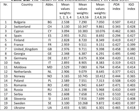
Fig. 3.1. The position of the European countries t after Mean(Xt ; s (1)
).
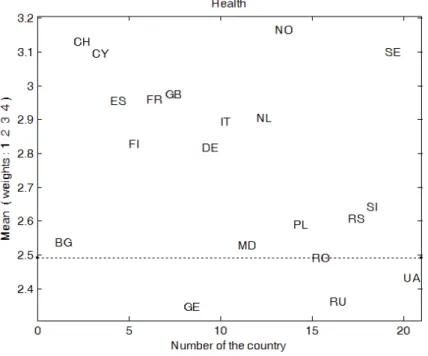
Fig. 3.2. The position of the European countries t after Mean(Xt ; s (2)
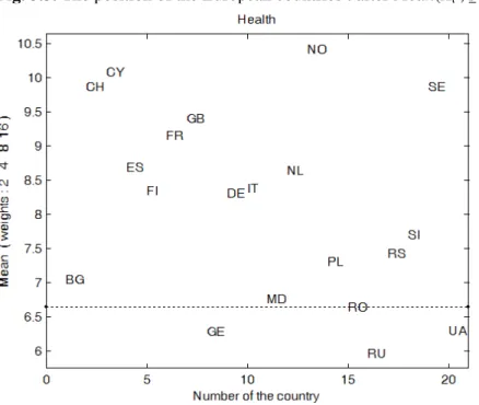
Fig. 3.3. The position of the European countries t after Mean(Xt ; s (3)
).
Without having a linear relationship between the weights s(1) , s(2) , s(3) attached to the ordinal classes of variables Xt and ignoring the measurement scale, we observe that Fig. 3.1-3.3 are very similar. This may result
from a structural similarity of the distributions of the answers in the European countries t, which are involved in the current statistical analysis. Theoretically, the means Mean(Xt ; s
(j)
) have, in general, distinct values compared with the used scores s(1) , s(2) , s(3).
Considering the means Mean(Xt ; s (j)
) , 1 j 3, Tables 3.4-3.6 establish the hierarchy between the studied countries t, 1 t 20.
Table 3.4. The hierarchy of the European countries t considering Mean(Xt ; s(1)).
Rank 1 2 3 4 5 6 7 8 9 10
Country NO CH SE CY GB FR ES NL IT FI
Mean 3.165 3.130 3.100 3.094 2.976 2.959 2.955 2.906 2.893 2.828
Rank 11 12 13 14 15 16 17 18 19 20
Country DE SI RS PL BG MD RO UA RU GE
Mean 2.817 2.643 2.608 2.589 2.538 2.529 2.492 2.433 2.363 2.348
Table 3.5. The hierarchy of the European countries t considering Mean(Xt ; s (2)
).
Rank 1 2 3 4 5 6 7 8 9 10
Country NO CY CH SE GB FR ES NL IT FI
Mean 10.745 10.383 10.347 10.268 9.711 9.511 9.251 9.079 8.905 8.720
Rank 11 12 13 14 15 16 17 18 19 20
Country DE SI RS PL BG MD RO UA GE RU
Mean 8.675 7.916 7.658 7.551 7.290 7.083 6.941 6.581 6.387 6.198
Table 3.6. The hierarchy of the European countries t considering Mean(Xt ; s (3)
).
Rank 1 2 3 4 5 6 7 8 9 10
Country NO CY SE CH GB FR ES NL IT FI
Mean 10.412 10.076 9.872 9.861 9.398 9.151 8.692 8.645 8.383 8.349
Rank 11 12 13 14 15 16 17 18 19 20
Country DE SI RS PL BG MD RO UA GE RU
Mean 8.304 7.699 7.423 7.313 7.050 6.764 6.647 6.301 6.291 5.968
Comparing Tables 3.4-3.6 we observe the following:
Maria Livia Ştefănescu 63
Romania is always situated on the 17th place out of the 20 countries considered. Georgia, Ukraine and Russia are the only countries that are situated below Romania from the point of view of the health status of their corresponding population. Bulgaria and Moldova have a slightly better position than Romania.
Norway is on the first place in all three variants of scores s. On the last place we find Russia, no matter what scores s are used.
Regarding the different scores s attributed to the ordinal classes, the places 2-4 from the classification are divided between Cyprus, Sweden and Switzerland.
The averages resulted from the three hierarchies differ sometimes significantly with respect to the scores s.
4. Polarization coefficient
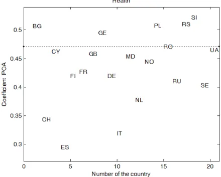
We will attempt to produce a hierarchization of the 20 European countries taking under account the polarization of answers from the population regarding the individual health status. Concretely, in Fig 4.1 we represent graphically the position of the countries t , 1 t 20 , with respect to POA(Xt) the degree of
bipolarization of the ordinal variables Xt . The values of POA(Xt) can be found in Table 2.2.
Fig. 4.1. The position of the European countries t using the values POA(Xt).
Taking into account the polarization level of the population’s answers we obtain in Table 4.2 a new
hierarchization of the European states.
Table 4.2. The hierarchy of the European countries t based on POA(Xt).
Rank 1 2 3 4 5 6 7 8 9 10
Country ES IT CH NL SE RU FI DE FR NO
POA 0.294 0.319 0.343 0.377 0.403 0.410 0.419 0.420 0.427 0.444
Rank 11 12 13 14 15 16 17 18 19 20
Country MD GB CY UA RO GE BG PL RS SI
POA 0.454 0.458 0.462 0.465 0.471 0.495 0.507 0.508 0.510 0.522
Analyzing the graphical representation from Fig. 4.1, as well as the data from Table 4.2, we mention the following:
The new hierarchy given by Table 4.2 differs significantly from the hierarchies in Tables 3.4-3.6. Taking into account, the polarization degree of answers to question Q1 , Romania is situated on
This time, besides Georgia, we find a polarization that is higher than Romania’s in: Bulgaria, Poland, Serbia and Slovenia.
From the studied countries, Slovenia presents the highest degree of polarization of the
population’s answers.
Compared to the hierarchizations from Tables 3.4-3.6, in the new classification Russia and
Ukraine have a lower polarization than România. The smallest polarization is found in Spain and Italy.
Norway is on the 10th place when it comes to the polarization index. In the previous hierarchizations, which used the mean indicator, Norway was on the first place.
Taking into account the mean criterion or the value of the bipolarization index, Romania is situated on an inferiour position, that is in the last quarter of the studied countries.
5. Inequality indicator
In this section, we will use a new coefficient of hierarchization, that is the inequality degree which is present in the answers of the population at question Q1.
Concretely, we will use for the hierarchization the values of the indicator IGO , which were presented in
Table 2.2.
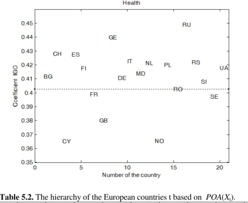
Fig. 5.1 gives us a suggestive graphical image regarding the positioning of the European countries with respect to the IGO level of inequality.
By making a synthetical presentation, Table 5.2 suggests a hierachization of the 20 countries studied regarded the inequality appeared in the distribution of answers of the persons interviewed.
By interpreting Fig. 5.1 and the data from Table 5.2 we observe the following :
The hierarchy based on the value of the indicator IGO of inequality differs significantly from all the previous classifications ( to compare Tables 3.4-3.6, 4.2 with Table5.2 ).
Regarding the level of inequality of the distribution of answers to question Q1, Romania has a top position, that is place 6 out of 20 countries. In the previous classifications, Romania had one of the last places.
With an inequality coefficient smaller than Romania’s, we find the following five countries: Cyprus, Norway, United Kingdom, France and Sweden.
Cyprus is the country in which the inequality of the answers’ distribution is the smallest.
Georgia and Russia are positionned on the final two places regarding the inequality degree. Norway and Spain who were on the first place in the preceeding classifications are now on the
2nd place and 17 place respectively. A very small polarization in Spain is superposed over a very
high inequality for the population’s answers.
This last classification based on the inequality phenomenon seems unrealistic in many situation. See for example the cases of Romania and Spain.
When referring to the population’s opinion regarding the individual health status, for many
Maria Livia Ştefănescu 65
Fig. 5.1. The position of the European countries t using the values IGO(Xt).
Table 5.2. The hierarchy of the European countries t based on POA(Xt).
Rank 1 2 3 4 5 6 7 8 9 10
Country CY NO GB SE FR RO SI DE BG MD
IGO 0.365 0.365 0.380 0.397 0.399 0.403 0.408 0.411 0.412 0.414
Rank 11 12 13 14 15 16 17 18 19 20
Country FI UA PL NL RS IT ES CH GE RU
IGO 0.417 0.418 0.420 0.421 0.422 0.423 0.427 0.428 0.440 0.449
6. Final conclusions
We do not recommend for SAH data to be used the mean indicator, because in the case of ordinal variables the attribution of subjective scores s attached to the classes does not have a theoretical basis. In the situation that we have presented, there are no significant fluctuations in the ordering of the studied European countries. (
Table 3.4-3.6 ). Romania is constantly on the 17th place out of the 20 countries.
Evidently, the resulting classification depends on the applied criterion ( Tables3.4-3.6, 4.2, 5.2 ) . We have used three indicators for the hierarchization of the European states, that are the following: evaluation index for the mean, polarization coefficient, inequality coefficient. ( Fig. 3.1-3.3, 4.1, 5.1 ).
It is preferable that the countries hierarchization is not made by using a single criterion. The polarization and inequality criterion are distinct, a fact that is shown by the values of the indicators POA and IGO respectively (
Table 2.2 ). In fact, the indicators POA and IGO are independent ( Ştefănescu [10] , Table 4.1 and Graphic 4.2 ). The hierarchization of the countries using separately the three indicators are sometimes very different ( Tables 3.4-3.6, 4.2 , 5.2 ). This fact determines distinct positionings for Romania in regard to the used indicators.
In order to obtain a more precise classification, we propuse the simultaneous use of the two indicators POA
and IGO by creating an aggregate indicator.
References
[1] Agresti, A., “An introduction to categorical data analysis”, Wiley Interscience, New Jersey, second edition, 2007. [2] Apouey, B., “Measuring health polarization with self-assessed health data”, Health Economics, 16 (9), pp.875–894, 2007. [3] Berry, K.J., Mielke, P.W., “Indices of ordinal variation”, Perceptual and Motor Skills, 74, pp. 576-578, 1992.
[4] Blair, J., Lacy, M.G., “Measures of variation for ordinal data as functions of the cumulative distribution”, Perceptual & Motor Skills, 82(2), pp. 411-418, 1996.
[6] Cowell, F.A., Ebert, U., “Complaints and inequality”, Social Choice and Welfare, 23, pp. 71-89, 2004. [7] Cowell, F.A., “Measuring Inequality”, Oxford University Press, Oxford, 2011 (third edition).
[8] Cowell, F.A., Flachaire, E., “Inequality with ordinal data”, STICERD London School of Economics, Aix-Marseille University, Working paper, pp. 1-50, October 2014.
[9] Giudici, P., Raffinetti, E., “A Gini concentration quality measure for ordinal variables”, Quaderni del Dipartimento di Economia, Statistica e
Diritto, Università di Pavia, Serie Statistica, pp. 1-18, no. 1/2011 (April 7, 2011).