A hierarchical neural model in short-term load forecasting
Otavio A.S. Carpinteiro
a,∗, Agnaldo J.R. Reis
a, Alexandre P.A. da Silva
baResearch Group on Computer Networks and Software Engineering, Federal University of Itajubá,
Av. BPS 1303, Itajubá, MG 37500-903, Brazil
bPEE-COPPE, Federal University of Rio de Janeiro, CP 68504, Rio de Janeiro, RJ 21945-970, Brazil
Received 25 February 2003; received in revised form 3 June 2003; accepted 11 February 2004
Abstract
This paper proposes a novel neural model to the problem of short-term load forecasting (STLF). The neural model is made up of two self-organizing map (SOM) nets—one on top of the other. It has been successfully applied to domains in which the context information given by former events plays a primary role. The model was trained on load data extracted from a Brazilian electric utility, and compared to a multilayer perceptron (MLP) load forecaster. It was required to predict once every hour the electric load during the next 24 h. The paper presents the results, the conclusions, and points out some directions for future work. © 2004 Elsevier B.V. All rights reserved.
Keywords:Short-term load forecasting; Self-organizing map; Neural network
1. Introduction
With power systems growth and the increase in their complexity, many factors have become influential to the electric power generation and consumption (e.g., load management, energy exchange, spot pricing, in-dependent power producers, non-conventional energy, generation units, etc.). Therefore, the forecasting pro-cess has become even more complex, and more ac-curate forecasts are needed. The relationship between the load and its exogenous factors is complex and non-linear, making it quite difficult to model through conventional techniques, such as time series and linear regression analysis. Besides not giving the required precision, most of the traditional techniques are not ro-bust enough. They fail to give accurate forecasts when
∗Corresponding author.
E-mail addresses:[email protected] (O.A.S. Carpinteiro), [email protected] (A.J.R. Reis), [email protected] (A.P.A. da Silva).
quick weather changes occur. Other problems include noise immunity, portability and maintenance[1].
Neural networks (NNs) have succeeded in several power system problems, such as planning, control, analysis, protection, design, load forecasting, security analysis, and fault diagnosis. The last three are the most popular[2]. The NN ability in mapping complex non-linear relationships is responsible for the growing number of its application to the short-term load fore-casting (STLF)[3–6]. Several electric utilities over the world have been applying NNs for load forecasting in an experimental or operational basis[1,2,4].
So far, the great majority of proposals on the appli-cation of NNs to STLF use the multilayer perceptron (MLP) trained with error backpropagation. Besides the high computational burden for supervised train-ing, MLPs do not have a good ability to detect data outside the domain of the training data.
This paper introduces a new hierarchical neural model (HNM) to STLF. The HNM is an extension of the Kohonen’s original self-organizing map (SOM)
[7]. Several researchers have extended the Kohonen’s self-organizing feature map model to recognize se-quential information. The problem involves either recognizing a set of sequences of vectors in time or recognizing sub-sequences inside a large and unique sequence.
Several approaches, such as windowed data ap-proach[8], time integral approach1 [9], and specific approaches[10]have been proposed in the literature. Many of these approaches have well-known defi-ciencies[11]. Among all, loss of context is the most serious.
The proposed model is a hierarchical model. The hierarchical topology yields to the model the power to process efficiently the context information embedded in the input sequences. The model does not suffer from loss of context. On the contrary, it holds a very good memory for past events, enabling it to produce better forecasts. It has been applied to load data extracted from a Brazilian electric utility, and compared to a MLP model.
This paper is divided as follows. The second sec-tion provides an overview of related research. The third section presents the data representation. In the fourth and fifth sections, the load forecasting models and their training processes are respectively discussed. The sixth section explains the HNM output mapping process. The models are compared through forecast-ing simulations in the seventh section. The last sec-tion presents the main conclusions of the paper, and indicates some directions for future work.
2. Related research
The importance of STLF has been increasing lately. With deregulation and competition, energy price casting has become a valuable business. Bus-load fore-casting is essential to feed analytical methods uti-lized for determining energy prices. The variability and non-stationarity of loads are becoming critical owing to the dynamics of energy prices. In addition, the number of nodal loads to be predicted does not allow frequent interactions with load forecasting ex-perts. More autonomous load predictors are needed in the new competitive scenario.
1 Also known as leaky integral approach.
Artificial NNs have been successfully applied to STLF. Many electric utilities, which had previ-ously employed STLF tools based on classical sta-tistical techniques, are now using NN-based STLF tools.
Park et al.[6]have successfully introduced an ap-proach to STLF which employs a NN as main part of the forecaster. The authors employed a feed-forward NN trained with the standard error back-propagation (EBP) algorithm. Three NN-based predictors have been developed and applied to short-term forecast-ing of daily peak load, total daily energy, and hourly daily load, respectively. Three months of actual load data from Puget Sound Power and Light Company have been used in order to test the aforementioned forecasters. Only ordinary weekdays were taken into consideration for the training data.
Another successful example of NN-based STLF can be found in Lee et al.[12]. The authors employed a MLP trained with EBP to predict the hourly load for a lead time of 1–24 h. Two different approaches have been considered, namely one-step ahead forecasting (named static approach), and 1–24 steps ahead (named dynamic approach). In both cases, the load was sep-arated in weekday (Tuesdays through Fridays) and weekend loads (Saturdays through Mondays).
Bakirtzis et al. [4] employed a single fully con-nected NN to predict, on a daily basis, the load along a whole year for the Greek power system. The au-thors made use of the previous year for training pur-poses. Holidays were excluded from the training set and treated separately. The network was retrained daily using a moving window of the 365 most recent in-put/output patterns. More, the paper proposed another procedure to 2–7 days ahead forecasting.
evaluates the operation of a neural model in a realistic electrical utility environment.
Khotanzad et al.[14]describe the third generation of an hourly STLF system, named artificial neural net-work short-term load forecaster (ANNSTLF). Its ar-chitecture includes only two neural forecasters—one forecasts the base load, and the other predicts the change in load. The final prediction is obtained via adaptive combination of these two forecasts. A novel scheme for forecasting holiday loads is developed as well. The performance on data from ten different util-ities is reported and compared to the previous gener-ation forecasting system.
Finally, a comprehensive review of the application of NNs to STLF can be found in Hippert et al. [15]. The authors examine a collection of papers published between 1991 and 1999.
3. Data representation
This section introduces the data representation em-ployed on the input layers of the load forecasting neu-ral models. The input data consisted of sequences of load data extracted from a Brazilian electric utility. Different representations were tried out on each model. The representations presented below produced the best results for each model.
3.1. Data representation for HNM
Seven neural input units are used in the representa-tion, as shown inTable 1. The first unit represents the load at the current hour. The second, the load at the hour immediately before. The third, fourth and fifth units represent respectively the load at 24 h behind, at 1 week behind, and at 1 week and 24 h behind the hour whose load is to be predicted. The sixth and seventh units represent a trigonometric coding for the hour to
Table 1
Input variables for the HNM model
Input Variable name Lagged values (h)
1–5 Load (P) 1, 2, 24, 168, 192
6 HS 0a
7 HC 0a
aLag 0 represents the hour to be forecast.
Table 2
Input variables for the MLP model
Input Variable name Lagged values (h)
1–4 Load (P) 1, 2, 24, 168
5 HS 0a
6 HC 0a
aLag 0 represents the hour to be forecast.
be forecast, i.e., sin(2π·hour/24) and cos(2π·hour/24). Each unit receives real values. The load data is prepro-cessed using ordinary normalization (minimum and maximum values in the [0, 1] range).
3.2. Data representation for MLP
The representation for the MLP is displayed in Table 2. It is quite similar to that employed on the input layer of the HNM. It includes all input units em-ployed in the representation for the HNM, except the unit which represents the load at 1 week and 24 h be-hind the hour whose load is to be predicted. Six units are thus used. The load values are also preprocessed using ordinary normalization.
4. Load forecasting models
This section describes the loading forecasting mod-els.
4.1. The HNM
The model is made up of two SOMs, as shown inFig. 1. Its features, performance, and potential are better evaluated in[16,17].
V(t) SOM
Bottom SOM Top
Time Integrator
Map Map
Time Integrator
Λ
The input to the model is a sequence in time of m-dimensional vectors, S1 = V(1),V(2), . . . ,
V(t), . . . ,V(z), where the components of each vector are real values. The sequence is presented to the input layer of the bottom SOM, one vector at a time. The input layer hasmunits, one for each component of the input vectorV(t), and a time integrator. The activation
X(t) of the units in the input layer is given by
X(t)=V(t)+δ1X(t−1) (1) whereδ1 ∈ (0,1) is the decay rate. For each input vector X(t), the winning unit i∗(t) in the map is the unit which has the smallest distanceψ(i,t). For each output uniti,ψ(i,t) is given by the Euclidean distance between the input vector X(t) and the unit’s weight vectorWi.
Each output unitiin the neighborhoodN∗(t)of the winning uniti∗(t)has its weightWi updated by
Wi(t+1)=Wi(t)+αΥ(i)[X(t)−Wi(t)] (2)
whereα∈(0,1)is the learning rate.Υ(i)is the
neigh-borhood interaction function [18], a Gaussian type
function, and is given by
Υ(i)=κ1+κ2e−κ3[Φ(i,i
∗(t))]2/2σ2
(3)
whereκ1,κ2, andκ3are constants,σis the radius of the neighborhoodN∗(t), andΦ(i, i∗(t))is the distance in the map between the unitiand the winning uniti∗(t). The distanceΦ(i′, i′′)between any two unitsi′andi′′
in the map is calculated according to the maximum norm,
Φ(i′, i′′)=max{|l′−l′′|,|c′−c′′|} (4)
where (l′, c′) and (l′′, c′′) are the coordinates of the unitsi′andi′′, respectively in the map.
The input to the top SOM is determined by the distancesΦ(i,i∗(t)) of then units in the map of the
bottom SOM. The input is thus a sequence in time of n-dimensional vectors, S2 = Λ(Φ(i, i∗(1))), Λ (Φ(i, i∗(2))), . . . , Λ(Φ(i, i∗(t))), . . . , Λ(Φ(i, i∗(z))), where Λ is a n-dimensional transfer function on a
n-dimensional space domain.Λis defined as
Λ(Φ(i, i∗(t)))=
1−κΦ(i, i∗(t)) ifi∈N∗(t) 0 otherwise
(5)
whereκis a constant, andN∗(t) is a neighborhood of the winning unit.
The sequenceS2is then presented to the input layer of the top SOM, one vector at a time. The input layer hasnunits, one for each component of the input vector Λ(Φ(i, i∗(t))), and a time integrator. The activation
X(t) of the units in the input layer is thus given by
X(t)=Λ(Φ(i, i∗(t)))+δ2X(t−1) (6) whereδ2∈(0,1)is the decay rate.
The dynamics of the top SOM is identical to that of the bottom SOM.
4.2. The MLP
One single hidden layer with one to three hidden neurons is used. An usual hyperbolic activation func-tion is adopted in the hidden layer. In the output layer, it is adopted a linear activation function. Only one unit is used on the output layer.
5. Training processes
This section describes the HNM and MLP training processes.
5.1. HNM training process
Two different HNMs are conceived. The first one is required to foresee the time horizon from the first to the sixth hour. This is due to the fact that the load series un-der consiun-deration presents two distinct periods—from the first to the sixth hour, and from the seventh to the 24th hour.
the memory for the former day predictions. The initial weights were given randomly to both SOMs.
The forecasting of the remaining time—seventh to 24th hour—is addressed by the second model. The same training process previously described is applied to this model too. Nevertheless, medium values for de-cay rates—0.5 and 0.8 for the bottom and top SOMs, respectively—were used instead. These new values for decay rates extend the memory size for past events [16], and consequently, yield more accurate predic-tions on large horizons.
The training set comprised 2160 load patterns, span-ning 90 days. They were taken from November 1994 to January 1995. The maximum electric load fell around 3900 MW. There was no particular treatment for hol-idays.
5.2. MLP training process
Six-week windows were taken for training, with data grouping according to the day of the week. For each day of the week, a MLP was trained, applying the backpropagation algorithm with cross-validation. Dif-ferent partitions for the training and testing sets were randomly created every 50 epochs.
The 24 load forecasts are computed after the one-step ahead training. The load forecasters are re-trained at the end of the day. The training window is then moved 1 day forward, and the forecasts for the next 24 h are performed.
The training set comprised the same 2160 load pat-terns employed on the HNM training process. There was no particular treatment for holidays, as well.
6. HNM output mapping process
The output of the top SOM of the HNM model rep-resent the forecast load. The forecast load produced by the top SOM at hourtcorresponds to the sequence of load patterns presented to the input layer of the bottom SOM until hour (t−1). Feedback is thus pos-sible at any moment, by presenting the forecast load at hour t to the input layer, in order to generate the forecast load at hour (t+1). This procedure is car-ried out 24 times, leading a recursive load forecast-ing scheme, rangforecast-ing from the first to the 24th hour ahead.
The training set is employed to map the HNM out-put. After the training phase, the training set is input again, pattern by pattern, in a sequence. As the load patterns in the training set are all known, it is possible to identify which activated areas in the map of the top SOM are associated with these patterns.
For instance, let the sequence of vectorsS=V(1),
V(2), . . . ,V(t), . . . ,V(z), be the representation of the load patterns P(1),P(2), . . . ,P(t), . . . ,P(z).
After inputtingV(1), a winning uniti∗(1) as well as the units in its neighborhood N∗(1) in the map are activated. The winning uniti∗(1) thus represents the forecast load at time 2, that is, the load patternP(2).
Following this mapping process, it is thus feasible to identify which winning unit is associated with a cer-tain load pattern, and then attach to that unit that load value. Such a process has nonetheless two weaknesses. First, it may be possible that a winning unit respond to more than one load pattern. In this case, it is at-tached to that unit the mean of the load values of those patterns.
Second, it may be possible that an unit never re-spond to any pattern, as well. In such case, it is attached to that unit the mean of the load values of the winning units in its neighbourhood. A new map-ping process which avoids these weaknesses is under development.
7. Results
The forecasts were performed on the HNM and MLP models. A comparison of both models was also performed. The mean absolute percentage error (MAPE), mean square error (MSE), mean error (ME), and maximum percentage error (MAX) were used to evaluate the models.
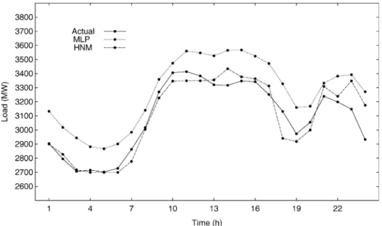
Figs. 2 and 3 show the actual load and forecast load for two particular days. The first one—Friday, 3 February 1995—is a typical weekday, and the second one—Tuesday, 7 February 1995—is a special week-day.
Fig. 2. Actual load and forecast load for 3 February 1995.
stationary behavior. Such holiday is then said to be a special weekday. Special weekdays break down fore-casters, for they perform much better on typical than on special weekdays.
Table 3presents the performance of the forecasters for 1–24 step ahead predictions on those weekdays. Table 4displays a global average evaluation for those days.
The results from the HNM are very promising. On the typical day, HNM performed better than MLP
Fig. 3. Actual load and forecast load for 7 February 1995.
on MAPE and MSE. In its turn, it performed worse than MLP on ME and MAX. The results presented in Table 3show that HNM yielded 13 better hourly per-centage errors, and 11 worse perper-centage errors than MLP.
Table 3
Hourly percentage error for 3 and 7 February 1995 Time (h) 3 February 7 February
MLP HNM MLP HNM
1 0.92 1.70 7.88 0.11
2 0.28 0.99 7.98 1.14
3 1.92 2.19 8.76 0.41
4 3.57 0.70 6.14 0.58
5 4.48 0.68 6.09 0.12
6 3.97 0.71 6.37 1.04
7 2.70 1.47 4.23 2.98
8 2.32 0.76 4.07 0.43
9 5.12 2.26 2.72 1.31
10 4.78 0.94 1.99 1.75
11 2.79 0.74 4.28 1.90
12 1.37 2.37 4.83 1.02
13 2.50 3.90 6.18 1.04
14 2.92 4.01 7.49 3.54
15 4.51 3.19 6.57 0.90
16 4.58 3.89 5.41 0.63
17 0.54 5.36 6.76 1.86
18 3.48 2.49 6.27 6.11
19 3.75 2.24 6.28 1.85
20 1.31 2.74 3.72 1.81
21 1.62 0.75 2.90 2.19
22 0.96 2.77 5.74 1.24
23 1.16 4.12 7.78 6.38
24 1.91 4.89 11.56 8.30
The superior performance displayed by HNM seems to be justified by its superior capacity to en-code context information from load series in time, and to memorize that information in order to produce better forecasts.
The forecasting errors were fairly high, however, even for the HNM model. The load patterns were di-vided into seven groups, each one corresponding to a specific weekday. An analysis of those groups of patterns was then performed. It was observed that the training patterns within each group did not share much
Table 4
Overall evaluation of the forecasters for 3 and 7 February 1995 Errors 3 February 7 February
MLP HNM MLP HNM
MAPE (%) 2.64 2.33 5.92 2.03
MSE (MW2) 10156 8675 36259 7885
ME (MW) −51.50 52.99 180.65 8.70
MAX (%) 5.12 5.36 11.56 8.30
similarity between themselves. More, the difference was significant when comparing them with the testing patterns. Another Brazilian electric utility was con-tacted to provide us with more relevant and enlarged sequences of load data.
8. Conclusion
The paper presents a novel artificial neural model to the problem of STLF. The model has a topology made up of two SOM networks, one on top of the other. It encodes and manipulates context information effectively.
Some conclusions may be drawn from the exper-iments. First, the knowledge representation proposed for the HNM inputs seems to be adequate. It supplied the model with the necessary information to make it produce correct predictions.
Second, the HNM performance on the forecasts was much better than that of the MLP. The results obtained have shown that the HNM was able to perform effi-ciently the prediction of the electric load in short fore-casting horizons.
Third, it is worth mentioning that MLP has been widely employed to tackle the problem of STLF so far. The results obtained thus suggest that HNM may offer a better alternative to approach such problem.
A research and development project for a Brazilian electric utility is under course. The research will focus on the effects of the HNM time integrators on the predictions in order to produce a better adaptability. Besides, it will focus on the study of its performance on larger load databases. The forecasts should also span a larger number of days in order to be more significant statistically.
Acknowledgements
This research is supported by CNPq, Brazil.
References
[2] H. Mori, State-of-the-art overview on artificial neural networks in power systems, in: M. El-Sharkawi, D. Niebur (Eds.), A Tutorial Course on Artificial Neural Networks with Applications to Power Systems, IEEE Power Engineering Society, 1996, Chapter 6, pp. 51–70.
[3] K. Liu, S. Subbarayan, R. Shoults, M. Manry, C. Kwan, F. Lewis, J. Naccarino, Comparison of very short-term load forecasting techniques, IEEE Trans. Power Syst. 11 (2) (1996) 877–882.
[4] A. Bakirtzis, V. Petridis, S. Klartzis, M. Alexiadis, A. Maissis, A neural network short-term load forecasting model for the Greek power system, IEEE Trans. Power Syst. 11 (2) (1996) 858–863.
[5] O. Mohammed, D. Park, R. Merchant, T. Dinh, C. Tong, A. Azeem, J. Farah, C. Drake, Practical experiences with an adaptive neural network short-term load forecasting system, IEEE Trans. Power Syst. 10 (1) (1995) 254–265.
[6] D. Park, M. El-Sharkawi, R. Marks Jr., L. Atlas, M. Damborg, Electric load forecasting using an artificial neural network, IEEE Trans. Power Syst. 6 (2) (1991) 442–449.
[7] T. Kohonen, Self-Organizing Maps, third ed., Springer-Verlag, Berlin, 2001.
[8] J. Kangas, On the analysis of pattern sequences by self-organizing maps, Ph.D. thesis, Laboratory of Computer and Information Science, Helsinki University of Technology, Finland, 1994.
[9] G.J. Chappell, J.G. Taylor, The temporal Kohonen map, Neural Netw. 6 (1993) 441–445.
[10] D.L. James, R. Miikkulainen, SARDNET: a self-organizing feature map for sequences, in: G. Tesauro, D.S. Touretzky, T.K. Leen (Eds.), Proceedings of the Advances in Neural
Information Processing Systems, vol. 7, Morgan Kaufmann, 1995.
[11] O.A.S. Carpinteiro, A hierarchical self-organizing map model for sequence recognition, Pattern Anal. Applic. 3 (3) (2000) 279–287.
[12] K. Lee, Y. Cha, J. Park, Short-term load forecasting using an artificial neural network, IEEE Trans. Power Syst. 7 (1) (1992) 124–132.
[13] A. Papalexopoulos, S. Hao, T. Peng, An implementation of a neural network based load forecasting model for the EMS, IEEE Trans. Power Syst. 9 (4) (1994) 1956–1962. [14] A. Khotanzad, R. Afkhami-Rohani, D. Maratukulam,
ANNSTLF—artificial neural network short-term load forecaster—generation three, IEEE Trans. Power Syst. 13 (4) (1998) 1413–1422.
[15] H. Hippert, C. Pedreira, R. Souza, Neural networks for short-term load forecasting: a review and evaluation, IEEE Trans. Power Syst. 16 (1) (2001) 44–55.
[16] O.A.S. Carpinteiro, A hierarchical self-organizing map model for pattern recognition, in: L. Caloba, J. Barreto (Eds.), Proceedings of the Brazilian Congress on Artificial Neural Networks 97 (CBRN 97), UFSC, Florianopolis, SC, Brazil, 1997, pp. 484–488.
[17] O.A.S. Carpinteiro, A hierarchical self-organizing map model for sequence recognition, in: L. Niklasson, M. Boden, T. Ziemke (Eds.), Proceedings of the International Conference on Artificial Neural Networks 98, Springer-Verlag, Skovde, Sweden, 1998, pp. 815–820.