Nova School of Business and Economics
Universidade Nova de Lisboa
Three Essays on Structural Breaks
Author:
Nuno
Sobreira
Advisor:
Luis
Catela Nunes
CONTENTS
1. Tests for Multiple Breaks in the Trend with Stationary or Integrated Shocks . 19
1.1 Introduction . . . 19
1.2 Joint Broken Trend Model . . . 22
1.2.1 Known Break Fractions . . . 23
1.2.2 Unknown Break Fractions . . . 28
1.2.3 Double Maximum Tests . . . 30
1.2.4 Sequential Tests and Estimation of the Number of Breaks . . . . 32
1.3 Disjoint Broken Trend Model . . . 34
1.3.1 Known Break Fractions . . . 35
1.3.2 Unknown Break Fractions . . . 38
1.4 Size and Power Simulations . . . 40
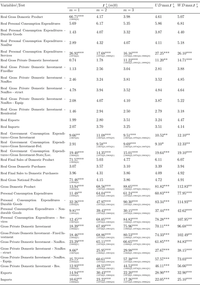
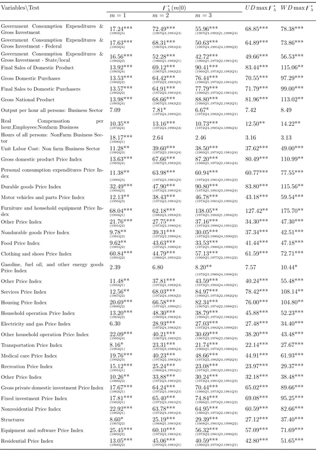
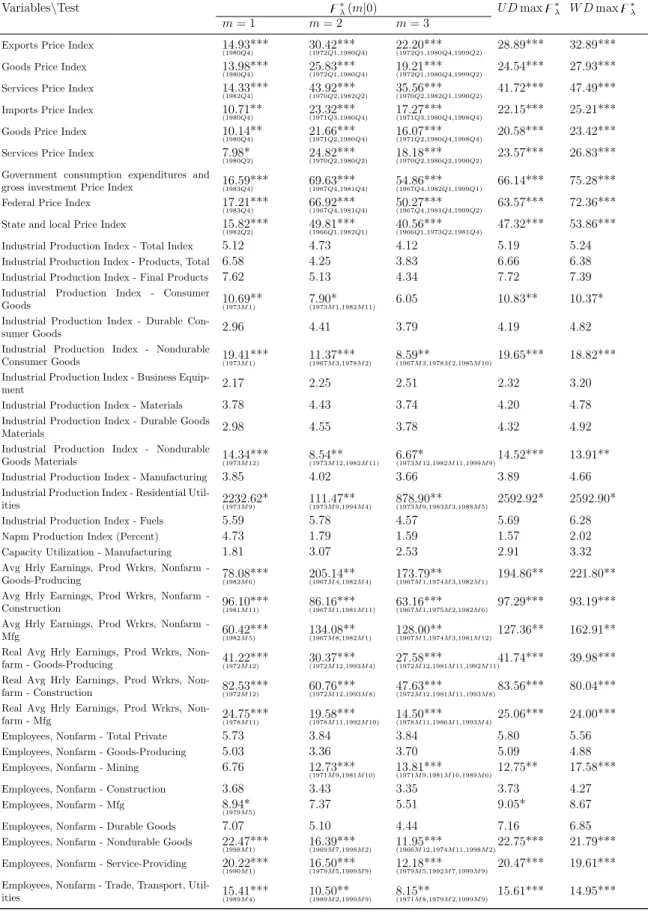
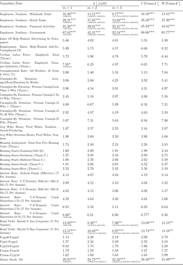
1.5 Empirical Application . . . 43
1.6 Conclusions . . . 45
2. Trend Breaks in Multivariate Time Series . . . 85
2.1 Introduction . . . 85
2.2 The Model and Assumptions . . . 91
2.3 The estimation method . . . 95
2.4 Testing for Common Breaks in Trend . . . 100
2.4.1 Known Break Fractions . . . 100
2.4.2 Unknown Break Fractions . . . 104
2.5 A test of l versus l+ 1 common broken trends . . . 107
2.6 Finite Sample Simulations . . . 110
2.8 Conclusion . . . 114
3. Neoclassical, semi-endogenous or endogenous growth theory? Evidence based on new structural change tests . . . 137
3.1 Introduction . . . 137
3.2 Assumptions and Methodology . . . 143
3.2.1 Econometric Model and Assumptions . . . 144
3.2.2 Detection and estimation of the number of breaks . . . 146
3.2.3 Testing for general linear restrictions on the trend function across regimes . . . 150
3.3 Results of the Economic Growth hypotheses tests . . . 155
3.3.1 Testing for Breaks in Steady State Growth . . . 156
3.3.2 Restricted Structural Breaks and Economic Growth hypotheses . 158 3.4 Conclusion . . . 160
LIST OF FIGURES
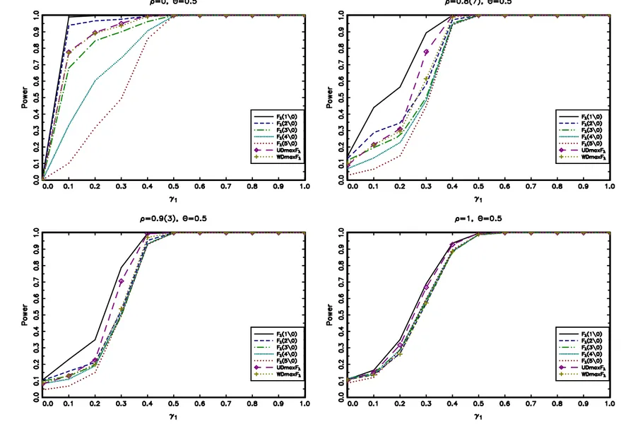
1.1 Power (1 break) of ̥∗
λ and Dmax̥∗λ tests, Model B, T=150 . . . 59
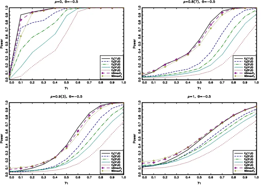
1.2 Power (1 break) of ̥∗
λ(m|0) and Dmax̥∗λ tests, Model B, T=150 . . . . 60
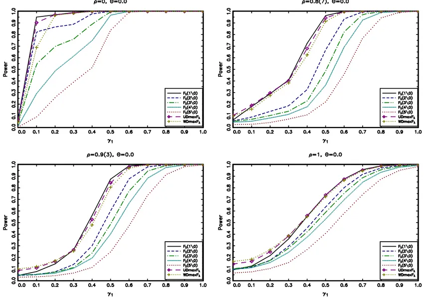
1.3 Power (1 break) of ̥∗
λ(m|0) and Dmax̥∗λ tests, Model B, T=150 . . . . 61
1.4 Various U.S. macroeconomic time series and estimated Model B break dates 72
1.5 Various U.S. macroeconomic time series and estimated Model B break
dates (continued) . . . 73
1.6 Various U.S. macroeconomic time series and estimated Model B break
dates (continued) . . . 74
1.7 Various U.S. macroeconomic time series and estimated Model B break
dates (continued) . . . 75
1.8 Various U.S. macroeconomic time series and estimated Model B break
dates (continued) . . . 76
1.9 Various U.S. macroeconomic time series and estimated Model B break
dates (continued) . . . 77
1.10 Various U.S. macroeconomic time series and estimated Model B break
dates (continued) . . . 78
1.11 Various U.S. macroeconomic time series and estimated Model B break
dates (continued) . . . 79
1.12 Various U.S. macroeconomic time series and estimated Model B break
dates (continued) . . . 80
1.13 Various U.S. macroeconomic time series and estimated Model B break
dates (continued) . . . 81
1.14 Various U.S. macroeconomic time series and estimated Model B break
1.15 Various U.S. macroeconomic time series and estimated Model B break
dates (continued) . . . 83
1.16 Sequential Tests procedure . . . 84
2.1 Top 1% Income shares for country groups with break dates detected with PQ (dotted) and Wλ (solid) methodologies . . . 130
3.1 Sequential Tests procedure . . . 170
3.2 Real GDP per capita - Western Europe . . . 171
3.3 Real GDP per capita - North/South America . . . 172
3.4 Real GDP per capita - Northern Europe . . . 173
3.5 Real GDP per capita - Asia and Oceania . . . 174
3.6 Real GDP per capita - Southern Europe . . . 175
LIST OF TABLES
1.1 Asymptotic critical values and bmξ values for the multiple trend breaks ̥∗ λ
and Double Maximum U Dmax̥∗
λ and W Dmax̥∗λ tests. . . 56
1.2 Asymptotic critical values andblξ values of the sequential trend breaks test
̥∗
λ(l+ 1|l) . . . 57
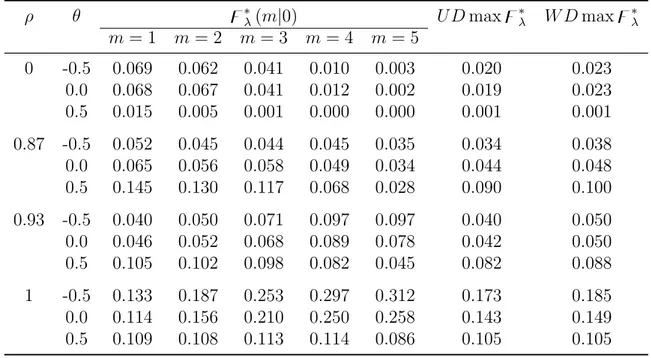
1.3 Empirical size of̥∗
λ(m|0) and Dmax̥∗λ tests, 5% nominal level, T = 150. 58
1.4 Size and Power of Sequential Tests, Model B, T=150 . . . 58
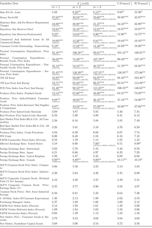
1.5 Empirical Application of ̥∗
λ and Dmax̥∗λ tests . . . 62
1.6 Empirical Application of ̥∗
λ and Dmax̥∗λ tests (continued) . . . 63
1.7 Empirical Application of ̥∗
λ and Dmax̥∗λ tests (continued) . . . 64
1.8 Empirical Application of ̥∗
λ and Dmax̥∗λ tests (continued) . . . 65
1.9 Empirical Application of ̥∗
λ and Dmax̥∗λ tests (continued) . . . 66
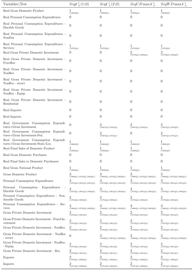
1.10 Empirical Application of Sequential tests to various U.S. macroeconomic
time series . . . 67
1.11 Empirical Application of Sequential tests to various U.S. macroeconomic
time series (continued) . . . 68
1.12 Empirical Application of Sequential tests to various U.S. macroeconomic
time series (continued) . . . 69
1.13 Empirical Application of Sequential tests to various U.S. macroeconomic
time series (continued) . . . 70
1.14 Empirical Application of Sequential tests to various U.S. macroeconomic
time series (continued) . . . 71
2.1 Asymptotic critical values of theWλ
∗ test statistic for the the 1 trend break
2.2 Asymptotic critical values for the sequential test Wλ(l+ 1|l). . . 128
2.3 Empirical size ofWλ(τ∗) test for τ∗ = 0.5, 5% nominal level . . . 128
2.4 Empirical size and power of Wλ test, 5% nominal level . . . 129
2.5 Group countries common trend breaks in the top 1% Income Share . . . 129
3.1 Empirical Application of ̥∗
λ and Dmax̥∗λ tests to real GDP per capita 167
3.2 Empirical Application of Sequential tests to real GDP per capita . . . 168
3.3 Restricted Structural Change Tests . . . 169
3.4 Estimated growth rates , in percentage terms, for the “growth shift”\“level
shift” hypothesis . . . 169
3.5 Estimated growth rates , in percentage terms, for the “growth shift”\“constant
trend” hypothesis . . . 169
ACKNOWLEDGMENTS
This doctoral thesis has been a long journey for me. It was a real privilege to participate
in it and I would like to express here my sincere thanks to all the people who contributed
to make this a successful experience.
Above all, I owe the most profound debt of gratitude to Professor Luis Catela Nunes for
his constant intellectual guidance, support, motivation and enthusiasm. Luis has always
been ready to read several drafts of this dissertation and provided several comments that
improved substantially its quality and helped this research project to constantly move
forward. Along these years, I also have benefited and learned greatly from numerous and
quite lengthy discussions with Luis about research problems and directions. I consider
that I have been truly very fortunate to have Luis as supervisor and it was and will
continue to be a real pleasure to work with him. I am also indebted to Professor Paulo
Rodrigues who helped to give a definite boost in the last chapter of this dissertation.
I want to express my appreciation and gratitude to Nova School of Business and
Economics for providing all the necessary conditions for this dissertation to be successful.
Although I officially started my Phd studies in September 2005, the first three years of
the program were mainly a crucial learning period. A special thanks goes to Professor
Iliyan Georgiev for truly shaping my mathematical mind and showing how apparently
very complex topics can be learned in a such a simple and clear manner.
I am also grateful to Instituto Superior T´ecnico, for their hospitality and permission
to do course work. In particular, I would like to thank Professor Ant´onio Pacheco,
Cl´audia Pascoal and Leonor Fernandes for their important support and motivation at
the beginning of this dissertation. I would like to thank Professor Peter Boswijk, Paulius
Stakenas, Yang Zu, Zhengyuan Gao and Simon Broda for their hospitality and helpful
During the Phd, I have been lucky to come across many good friends without whom
this period would have been much less enjoyable. In this context, it has been a real
pleasure to interact closely with Pedro Chaves, S´onia F´elix, Bernardo Pimentel, Mafalda
Sampaio, Nuno Paix˜ao, Erica Marujo, Doruk Iris, Tiago Botelho, David Henriques,
Ro-drigo Araujo, Vladimir Otrachshenko and Tymur Gabuniya who always provided a
stimu-lating, relaxed and well humored research environment. Other friends I must mention are
Nuno Godinho, Filipa Andreia, Andr´e Barata and Jo˜ao Sousa. Your constant presence,
dynamism and fellowship have always been very important throughout this period.
Financial support from Funda¸c˜ao para a Ciˆencia e Tecnologia (Doctoral Scholarship
SFRH / BD / 23658 / 2005) andFunda¸c˜ao Am´elia de Mello are also acknowledged.
Finally, I would like to dedicate my Phd Thesis to my parents and to Sandra Farropas
for their endless love, patience, encouragement and understanding at all times. There
are not enough words to express all the thanks you deserve for everything that you have
done and passed.
INTRODUCTION
This dissertation consists of three essays that propose robust statistical procedures for
testing hypotheses on the slope of the trend function. It includes statistics to test and
estimate the number and timing of breaks in the slope of the deterministic trend from
a univariate time series and from a multivariate time series robust to stationary,
non-stationary and cointegrated environments and robust tests for general linear restrictions
in the coefficients of trend, given the estimated regimes.
Structural changes are pervasive in economics: Changes in economic policy, evolving
technological progress or specific events with a strong impact in the World economy such
as wars or oil price shocks can give rise to structural breaks in any econometric model used
to explain the behavior of certain economic variables. On the other hand, the presence
of at least one structural break leads to inconsistent estimates and poor forecasts if that
break is not properly modeled. Naturally, this fact has led to a large amount of interest
on the literature about this topic. Different statistical procedures were proposed to test
for the existence of structural breaks and estimate both the number and timing of the
change points. The problem is that the majority of these tests are valid only when the
data are stationary. This fact restricts the applicability of these tests as, in practice, it
is rarely known as to whether the data are stationary or not. However, the literature on
multiple structural breaks valid in both I(0) and I(1) environments is relatively scarce.
This is a very important problem since in fact formal testing of whether a time series
contains structural breaks or not depend on whether the stochastic part is stationary or
not.
Hence, in the first chapter of my thesis, we propose new tests for the presence of
multiple breaks in the slope of the deterministic trend of a univariate time-series where
stationary or unit root shocks. These tests can also be used to sequentially estimate the
number of breaks. After developing the asymptotic theory and showing that the tests
work well for finite samples, we illustrate the applicability of the proposed tests to various
U.S. historical macroeconomic time series. Here we show how important it is to take into
account both the (non) stationarity of the data and the possible presence of multiple
breaks. We conclude that many macroeconomic variables are characterized by having
multiple breaks in the deterministic trend and not only one break as is very popularly
advocated in the literature.
The second chapter extends these ideas to the multivariate framework. This extension
is important for many reasons: first, intuitively many factors that may be responsible for
the presence of a structural break in a univariate time series may, by contagion, result
in structural changes in other economic variables. Second, the same circular problem
be-tween unit root and trend break testing can also be encountered within the cointegration
testing framework. Finally, it has been shown that we can expect substantial payoffs
in identifying, precisely, the dates in which breaks have occurred if we estimate them
in a multivariate system. Hence, in this chapter, we develop the first procedure which
delivers tests for the presence of common broken trends in multivariate time series which
do not require knowledge of the form of serial correlation in the data and are robust as
to whether the shocks are stationary, non stationary, cointegrated or not cointegrated.
The setup is a VAR process for cointegrated variables. We propose tests to detect and
estimate the number of change points occurring at known and unknown dates in a system
of equations. These tests are simple to implement and can be used to specify the
deter-ministic component of VAR Models. We present Monte Carlo simulation results which
suggest that the proposed tests perform well in small samples. The proposed
methodol-ogy is used to study the existence of trend breaks in data related to economic inequality.
In particular, we use a recently compiled database on the concentration of wealth in the
richest individuals. Here we identify those international economic events that were
re-sponsible for a change in the historical trend of concentration of wealth in various groups
of countries close to each other geographically and culturally.
The third chapter of this dissertation contributes to one of the prevalent topics in
the economic growth literature: the choice of the growth model more compatible with
what we observe in the data. An important part of this discussion can be summarized
in three mutually exclusive hypotheses: the “constant trend”, “level shift” and “slope
shift” hypothesis. The objective of this chapter is to classify countries according to each
of these hypotheses and to analyze which of the growth theories seems to be favored. We
approach this problem in two-steps: first, the number and the timing of trend breaks
are estimated using the approach from the first chapter; and second, conditional on the
estimated number of breaks, break dates, and coefficients, a statistical framework is
in-troduced to test for general linear restrictions on the coefficients of the linear disjoint
broken trend model. Here, we prove a general result that, under certain conditions, a
standard F statistic to test the additional restrictions, given the first step estimated
par-tition, converges asymptotically in distribution to the usual chi-square distribution. We
further show how the aforementioned hypotheses can be formulated as linear restrictions
on the parameters of the breaking trend model and apply the methodology to per capita
output of an extensive list of countries. All of our tests are robust as to whether the data
are I(0) or I(1) surpassing technical and methodological concerns on previous empirical
evidence. We find evidence favoring the “constant trend” hypothesis for nine countries:
Austria, Germany, Switzerland, Canada, United States, Chile, Sweden, Australia and
New Zealand. The results of our tests support the “level shift” hypothesis for six
coun-tries: France, Netherlands, Brazil, Denmark, Japan and Italy. Finally, there is a third
group of eight countries where statistical evidence favors the “growth shift” hypothesis:
Belgium, Uruguay, Finland, Norway, United Kingdom, Sri Lanka, Portugal and Spain.
All in all, this dissertation contributes to the literature of structural breaks by
propos-ing a different set of procedures that can be used in a univariate or in a multivariate
framework to detect both the number and timing of significant structural changes in the
trend function of one or multiple economic variables. This framework also allows to test
general linear restrictions on the trend, given the estimated partition. The advantage of
of a unit root or specify the number of cointegrating relations to solve this statistical
inference problem. Empirical applications show that it is important to take into account
these breaks as they are common in macroeconomic time series.
1. TESTS FOR MULTIPLE BREAKS IN THE TREND WITH
STATIONARY OR INTEGRATED SHOCKS
With Luis C. Nunes1
1.1
Introduction
Many macroeconomic time series are characterized by a clear tendency to grow over
time, that is, as having a deterministic time trend component. There has been a large
debate in the literature regarding the appropriate methods to infer about the linearity
and stability of the trend function and the nature of the shocks affecting a time series.
This is a particularly important issue when it comes to make accurate economic forecasts
or test economic hypothesis. In fact, there are many interesting economic applications
that involve statistical inference on the parameters of the trend function, namely, in the
continuous time macroeconomic modeling (see Bergstrom et al., 1992, Nowman, 1998), in
international trade, for example, with the Prebish-Singer hypothesis testing (see Bunzel
and Vogelsang, 2005), in the empirical debate regarding regional convergence in per capita
income (see Sayginsoy and Vogelsang, 2004), or in environmental economics on the future
consequences of global warming (see Vogelsang and Franses, 2005).
The stationarity properties of the shocks have important implications on the
appro-priate methods to make inferences about the trend function. In particular, the correct
approach to make inferences about the stability or the existence of breaks in the trend
1We are grateful to participants in seminars at Universiteit Van Amsterdam and Nova School of
depends on whether the shocks are I(0) or I(1). In the first case one should use regressions
on the levels, while for the latter the correct approach is to model the first-differences
of the series. However, it is often not known a priori whether the shocks are stationary
or contain a unit-root. Moreover, stationarity or unit-root tests also suffer from similar
problems since their properties are in turn affected by the stability of the trend function.
Only recently have some solutions to this dilemma been proposed in the literature.
These resort to statistical tests of the null hypothesis of a constant linear trend against the
alternative of a one break at some unknown date that do not require a priori knowledge
of whether the noise is I(0) or I(1). Sayginsoy and Vogelsang (2004) proposed a Mean
Wald and a Sup Wald statistic scaled by a factor based on unit root tests to smooth
the discontinuities in the asymptotic distributions of the test statistics as the errors
go from I(0) to I(1). The scaling factor approach is based on Vogelsang (1998) who
proposed test statistics for general linear hypothesis regarding the parameters of the
trend function which do not require knowledge as to whether the innovations are I(0)
or I(1). Perron and Yabu (2009) proposed a Feasible Quasi Generalized Least Squares
approach to estimate the slope of the trend function. By truncating the estimate of the
sum of the autoregressive coefficients of the disturbance term to take the value of one
whenever the estimate is in a neighborhood of one, they have shown that the limiting
distribution of the t-statistic becomes Normal regardless of the persistence of the error
term. Kejriwal and Perron (2010) proposed a sequential testing procedure based on
Perron and Yabu (2009). Harvey et al. (2009) (hereafter HLT) employed a weighted
average of the appropriate regression t-statistics used to test the existence of a broken
trend when the errors are I(0) and I(1). However, as Lumsdaine and Papell (1997) point
out with an example of Jones (1995), allowing for only one break is not always the best
characterization of a macroeconomic variable, specially when analyzing long historical
time series.
This paper extends the results from HLT by providing tests of the null hypothesis of
no trend breaks against the alternative of one or more breaks in the trend slope which
do not require knowledge of the form of serial correlation in the data and are robust as
to whether the underlying shocks are stationary or have a unit-root. We build on the
framework proposed by HLT for the case of a single break, and construct test statistics
that are weighted averages of the appropriate F-statistics to test the existence of multiple
trend breaks when the disturbance term is I(0) and I(1).We adopt the weight function
used in HLT and prove that it has the same large sample properties regardless of the
number of trend breaks being tested.
We start by considering the case where the true break fractions are known and prove
that the proposed statistics converge in distribution to a chi-square distribution under
the null. Next, we consider the case where the trend break fractions are unknown and
need to be estimated. We transform our statistic in the same spirit as Andrews (1993)
and Bai and Perron (1998) and take the supremum of the F statistic over all possible
break fractions except those that are actively restricted by the trimming parameter. Here,
the weight function is evaluated at the estimated break fractions and we prove that its
large sample behavior is similar regardless of the number of break fractions estimated
and the number of structural breaks in the trend function. However, the asymptotic null
distributions of the appropriate F-statistics forI(0) and I(1) environments are different
and so, following Vogelsang (1998), we provide a scaling factor that makes the asymptotic
critical values invariant to the degree of persistence of the shocks. Finally, we propose
double maximum tests and a sequential test procedure that can be used to estimate
the number of trend breaks and that are also robust to the order of integration of the
error term. In both the known and unknown break dates settings, our proposed tests
are made robust to short memory serial correlation in the shocks via the use of standard
non-parametric estimators of the long run variance of the errors.
The outline of this article is as follows. Section 1.2 describes the multiple breaks in the
trend model, presents the test statistics for both known and unknown break fractions and
establishes the asymptotic behavior of these statistics. The sequential testing procedure
to estimate the number of breaks is also described. In Section 1.3 we extend the model
to allow for simultaneous shifts in the intercept and slope of the trend functions and
the application of the test statistics proposed, namely, the critical values and the choice
of the scaling constants. Size and power properties in finite samples from applying these
procedures are also discussed in this section. Section 1.5 provides an empirical application
to various U.S. macroeconomic time series data. Section 1.6 concludes the paper with
a discussion of some issues raised by our analysis and suggests possible paths for future
research. All our key results are proved in a Mathematical Appendix.
1.2
Joint Broken Trend Model
We start by considering a time-series process {yt} with a first-order linear trend and m
possible time changes in the slope such that the trend function is always joined at the
time of the break, which we call “Model A”:
yt =α+βt+ m
X
j=1
γjDTt τj∗
+ut, t = 1, . . . , T, (1.1)
and
ut=ρut−1+εt, t = 2, . . . , T, u1 =ε1, (1.2)
where DTt τj∗
:= ✶ t > Tj∗
t−Tj∗
captures the eventual jth break in the slope
oc-curring at date Tj∗ :=⌊τj∗T⌋with associated break fraction τj∗ ∈(0,1) and 0< τ1 < . . . <
τm <1. The slope coefficient changes fromβtoβ+γ1 at timeT1∗, fromβ+γ1 toβ+γ1+γ2
at time T2∗ and, in general, from β+
j−1
X
i=1
γi to β + j
X
i=1
γi at time Tj∗ for j = 1, . . . , m.
However, notice that the trend function is continuous in every period including the dates
at which the slope changes occur. The discontinuous case is considered in Section 1.3.
We assume that εt in (1.2) satisfies Assumption 1 of Sayginsoy and Vogelsang (2004,
pp. 2-3):
Assumption 1. The stochastic process εt is such that:
εt =C(L)ηt, C(L) = ∞
X
i=0
ciLi
with C(1)2 >0 and
∞
X
i=0
i|ci|< ∞, and where ηt is a martingale difference sequence with
unit conditional variance and sup
t
E ηt4<∞.
The error term ut can have one unit root or none. If |ρ| < 1, ut is an I(0) process.
But if ρ = 1 then ut turns out to be an I(1) process. We are interested in testing if
there are trend breaks in yt and in estimating the number of breaks in the time series
process, independently of whether ut is I(0) or I(1). Therefore, we would like to test
the null hypothesis H0 : γ1 = γ2 = . . . = γm = 0 against the two sided alternative:
H1 :γ1 6= 0∨γ2 6= 0∨. . .∨γm 6= 0.
Remark 1. Under the conditions of Assumption 1, the long run variance of εt is given
by ω2
ε := lim T→∞T
−1E T X t=1 εt !2
= C(1)2. In the I(0) case, the long run variance of ut is
given by ωu2 := lim
T→∞T −1E T X t=1 ut !2
=ωε2/(1−ρ)2.
1.2.1 Known Break Fractions
We start by considering the case where the vector of true break fractionsτ∗ = (τ1∗, τ2∗, . . . , τm∗)′ and hence all the eventual dates when the slope changes occur are known. The number
of breaks m is also known.
Similarly to HLT, we partition H1 into two local alternatives H1,0 :γ =κT−3/2 when
ut is I(0) and H1,1 : γ = κT−1/2 when ut is I(1) where γ = (γ1, γ2, . . . , γm)′ and κ is a
k-dimensional vector of finite non negative constants, κ= (κ1, κ2, . . . , κm)′.
Suppose one knows that ut is I(0), with ρ = 0 and εt is Gaussian white noise.
Then, to test the null hypothesis H0, we should use the standard F-statistic. Let
b
α,β,b bγ1(τ∗), . . . ,bγm(τ∗)
be the OLS estimators of the coefficients in equation (1.1)
andubt(τ∗) :=yt−αb−βtb − m
X
j=1
b
γj(τ∗)DTt τj∗
be the corresponding OLS residuals. Also
define xDT,t(τ∗) := {1, t, DTt(τ1∗), DTt(τ2∗), . . . , DTt(τm∗)} ′
as the vector of regressors.
The ̥0(τ∗) statistic is given by 2:
2The notation [.]
(i:j,i:j)([.](j)) is used to denote a submatrix (scalar) formed by rows and columns i
̥0(τ∗) =
b
γ(τ∗)′ bσ
2(τ∗)
" T X
t=1
xDT,t(τ∗)xDT,t(τ∗)′
#−1
(3:m+2,3:m+2)
−1
b
γ(τ∗)/m (1.3)
where bγ(τ∗) = (bγ1(τ∗),γb2(τ∗), . . . ,bγm(τ∗))′ with
b
γj(τ∗) =
T
X
t=1
xDT,t(τ∗)xDT,t(τ∗)′
!−1 T
X
t=1
xDT,t(τ∗)yt
(j+2)
, j = 1, . . . , m,
and bσ2(τ∗) := T−1
T
X
t=1
b
ut(τ∗)2.
Now suppose that ut is known to be I(1), with ρ = 1 and ∆ut is a Gaussian white
noise process. To test if the slope of the trend function is constant against the alternative
of m breaks over time we should use the F-statistic after differentiating the data. So by
applying first-differences to equation (1.1) we have:
∆yt=β+ m
X
j=1
γjDUt τj∗
+vt, t= 2, . . . , T (1.4)
where DUt τj∗
:= ✶ t > Tj∗ and vt = ∆ut. Let
e
β,eγ1(τ∗),eγ2(τ∗), . . . ,eγm(τ∗)
denote the OLS estimators of the parameters from (1.4) and vet(τ∗) = ∆yt − βe− m
X
j=1
e
γj(τ∗)DUt τj∗
the resulting residuals. Also letxDU,t(τ∗) :={1, DUt(τ1∗), DUt(τ2∗), . . . , DUt(τm∗)} ′
denote the vector of regressors. The ̥1(τ∗) statistic is given by:
̥1(τ∗) =γe(τ∗)′
eσ
2(τ∗)
" T X
t=2
xDU,t(τ∗)xDU,t(τ∗)′
#−1
(2:m+1,2:m+1)
−1
e
γ(τ∗)/m (1.5)
where eγ(τ∗) = (eγ1(τ∗),γe2(τ∗), . . . ,eγm(τ∗))′ with
e
γj(τ∗) =
T
X
t=2
xDU,t(τ∗)xDU,t(τ∗)′
!−1 T
X
t=2
xDU,t(τ∗) ∆yt
(j+1)
, j = 1, . . . , m,
and eσ2(τ∗) := (T −1)−1
T
X
t=2
e
vt(τ∗)2.
Remark 2. This paper is focusing its attention on the existence of multiple structural
breaks in the trend function. However, it is straightforward to adapt the test statistic to
other hypothesis of interest, for example, to test if the magnitude of the breaks was the
same in two different periods, or even non-linear hypothesis.
To accommodate more general forms of autocorrelation of the error terms as allowed
in Assumption 1, we simply substitute bσ2(τ∗) and σe2(τ∗) by non-parametric estimators of the long-run variances. Following Newey and West (1987), the following estimators
can be used:
b
ω2(τ∗) := bγ0(τ∗) + 2 l
X
j=1
h(j/l)bγj(τ∗), bγj(τ∗) = T−1 T
X
t=j+1
b
ut(τ∗)ubt−j(τ∗), (1.6)
and
e
ω2(τ∗) :=eγ0(τ∗) + 2 l
X
j=1
h(j/l)eγj(τ∗), eγj(τ∗) = (T −1)−1 T
X
t=j+1
e
vt(τ∗)evt−j(τ∗),
(1.7)
where the weights are given byh(j/l) := 1−j/(l+ 1) with lag truncationl =O(T1/4). In the sequel, unless otherwise stated, any reference to ̥0(τ∗) and̥
1(τ∗) will be taken
to imply those based on these long run variance estimators.
We now establish the asymptotic distribution of the ̥0(τ∗) and̥
1(τ∗) statistics. Theorem 1. Let the time series process be generated by (1.1) and (1.2), and let
(i) IfutisI(0) (|ρ|<1)then, underH1,0: (a)̥0(τ∗)−→d
1
mJ0(τ
∗, κ), and (b)̥
1(τ∗) =
Op l T , where
J0(τ∗, κ) ∼ χm2 (µ0), µ0=κ′
Q0(τ∗)/ω 2 u
κ,Q0(τ∗) = 1
Z
0
RT (r, τ∗)RT (r, τ∗)′dr
(ii) Ifut isI(1) (|ρ|= 1) then, underH1,1: (a)̥0(τ∗) =Op
T l
, and (b) ̥1(τ∗)−→d
1
mJ1(τ
∗, κ), where
J1(τ∗, κ) ∼ χm2 (µ1), µ1 =κ′
Q1(τ∗)/ω 2 ε
κ,Q1(τ∗) = 1
Z
0
RU (r, τ∗)RU (r, τ∗)′dr
The χ2m(µ) denotes the non-central chi-square distribution with m degrees of freedom and RT(r, τ∗) = (RT(r, τ1∗), RT(r, τ2∗), . . . , RT(r, τm∗))′ where RT(r, τi∗) is the contin-uous time residual from the projection of (r−τi∗)✶(r > τi∗) onto the space spanned by {1, r} and RU (r, τ∗) = (RU(r, τ1∗), . . . , RU(r, τm∗))′ where RU(r, τi∗) is the continuous time residual from the projection of ✶(r > τi∗) onto {1}.
Remark 3. From Theorem 1 we can easily conclude that, under H0 : γ = 0m×1 (or
κ = 0m×1), we have m·̥0(τ∗) d
−→ χ2m if ut is I(0) and also m·̥1(τ∗) d
−→ χ2m if ut
is I(1). If we knew all the true potential break dates and also the order of integration
of the error term ut, we could use the appropriate F-statistic to test if the potential m
changes in slope are statistically significant or not using critical values from the chi-square
distribution with m degrees of freedom. Also note that in the particular case of only one
break, m= 1, Theorem 1 is basically equivalent to Theorem 1 in HLT by the equivalence
between the F-statistic and the squared t-statistic when testing only one coefficient.
Remark 4. From the results of part (i) of Theorem 1 it is seen that when ut is I(0),
̥1(τ∗) converges in probability to zero, regardless of the value of κ. Similarly, from the
results in part (ii) of Theorem 1 it is seen that whenutis I(1),̥0(τ∗) diverges irrespective
of the value of κ.
Since, in practice, the order of integration is not known we would like to find a
pro-cedure that, at least asymptotically, converges to the asymptotic distribution of ̥0(τ∗)
when ut is I(0) and to the asymptotic distribution of ̥1(τ∗) when ut is I(1). More
specifically, we would like to find a weight function, call it λ(.), such that λ(.) −→p 1 if
ut is I(0) and λ(.) p
−→ 0 if ut is I(1) ensuring that the appropriate statistic with
non-degenerate distribution is selected. We employ the solution proposed by HLT and let
λ(.) be a function of the KPSS statistic of the original dataS0(τ∗) and of the differenced
data S1(τ∗) :
S0(τ∗) :=
PT
t=1
Pt
i=1ubi(τ∗)
2
T2ωb2(τ∗) , S1(τ ∗) :=
PT
t=2
Pt
i=1evi(τ∗)
2
(T −1)2ωe2(τ∗) (1.8) Lemma 1. Let the conditions of Theorem 1 hold:
(i) If ut is I(0), then: (a) S0(τ∗) = Op(1), and (b) S1(τ∗) =Op(l/T). (ii) If ut is I(1), then: (a) S0(τ∗) = Op(T /l), and (b) S1(τ∗) = Op(1).
Since by Lemma 1 the KPSS statistics, S0(τ∗) andS1(τ∗), have the same asymptotic
rates of convergence for a single or more trend breaks we can use the same weight function
from HLT:
λ(S0(τ∗), S1(τ∗)) := exp [− {gS0(τ∗)S1(τ∗)}v] (1.9)
whereg andv are positive constants. Now we are able to form the̥∗
λ statistic and study
its asymptotic distribution:
̥λ(τ∗) :={λ(S
0(τ∗), S1(τ∗))×̥0(τ∗)}+{[1−λ(S0(τ∗), S1(τ∗))]×̥1(τ∗)} (1.10)
Notice that a higher g gives more weight to ̥1 keeping everything else constant. Using the results from Theorem 1 and Lemma 1, we get the following result.
Corollary 1. Let the conditions of Theorem 1 hold.
(i) If ut isI(0), then: λ(S0(τ∗), S1(τ∗)) p
−→1 under bothH0 andH1,0, and ̥λ(τ∗) =
̥0(τ∗) +o p(1)
d
(ii) Ifut isI(1), then: λ(S0(τ∗), S1(τ∗)) p
−→0, under bothH0 andH1,1, and ̥λ(τ∗) =
̥1(τ∗) +o p(1)
d −→ 1
mJ1(τ
∗, κ).
Remark 5. From Corollary 1 we observe that we have constructed a test statistic to test
the presence ofm candidate trend breaks at known break dates that is valid regardless of
the order of integration of the errors. Ifut is I(0),̥λ(τ∗) is asymptotically equivalent to
̥0(τ∗), while if u
t is I(1), ̥λ(τ∗) becomes asymptotically equivalent to ̥1(τ∗). Since,
given these conditions, both m·̥0(τ∗) andm·̥
1(τ∗) converge in distribution to a
chi-square distribution withmdegrees of freedom under the null we can use the critical values
of the central chi-square distribution for̥λ(τ∗) irrespective of whether the disturbances,
ut, are I(0) or I(1).
1.2.2 Unknown Break Fractions
In this section, we consider tests of multiple structural changes in the trend function
with unknown change points. Suppose that the true break fractionsτ∗ are unknown but the number of breaks, m, is known. Proceeding in the same way as Andrews (1993)
and Bai and Perron (1998) we can form F type statistics to test the null hypothesis of
no trend breaks against the alternative hypothesis that there are m trend breaks. Let
τm := (τ1, . . . , τm) and Λm = {(τ1, . . . , τm) : |τi+1 −τi| ≥ η, τ1 ≥ η, τm ≤ 1−η} and
assume throughout that τ∗ ∈ Λm. If we knew that ut was I(0) the F-statistic would be
defined as:
̥∗
0(m|0) := sup τm∈Λm
̥0(τm) (1.11)
and if we knew thatut was I(1) the statistic would be given by:
̥∗
1(m|0) := sup τm∈Λm
̥1(τm), (1.12)
where the associated vectors of estimated break fractions of τ∗ are given by
b
τm := arg sup
τm∈Λm
̥0(τm) (1.13)
and
e
τm := arg sup
τm∈Λm
̥1(τm), (1.14)
respectively, such that̥∗
0(m|0) = ̥0(τbm) and̥∗1(m|0) =̥1(eτm). To solve the problem
of an unknown order of integration of the error term we follow the same strategy as in
the known break fraction case and write the analogue of the ̥λ(τ∗) statistic:
̥∗
λ(m|0) :={λ(τbm,τem)×̥∗0(m|0)}+bmξ {[1−λ(bτm,τem)]×̥∗1(m|0)} (1.15)
where λ(bτm,τem) := λ(S0(bτm), S1(eτm)) and bmξ is a positive finite constant such that,
as will be explained below, for any significance level ξ, the critical value of ̥∗ λ(m|0)
is the same regardless of whether ut is I(0) or I(1). The following Theorem states the
asymptotic distribution of ̥∗
0(m|0) and ̥∗1(m|0) under the null hypothesis γ = 0 when
the innovation sequence {ut} is either I(0) or I(1).
Theorem 2. Let the time series process be generated by (1.1) and (1.2) under H0 :γ = 0m×1 and let Assumption 1 hold.
(i) IfutisI(0), then: (a)̥∗0(m|0) d −→ 1
mτmsup∈Λm
J0(τm,0), and (b)̥∗1(m|0) =Op
l T
.
(ii) IfutisI(1), then: (a)̥∗0(m|0) =Op
T l
, and (b)̥∗ 1(m|0)
d −→ 1
mτmsup∈ΛmJ1(τ m,0).
Remark 6. HLT established the divergence rates for the 1 break case under a fixed
alternative H1 : γ 6= 0 using supt instead of sup̥ statistics. Since ̥i(τ1) = (ti(τ1))2
and ̥i(τ1)62̥i(τ1, τ2)6m̥i(τ1, . . . , τm), i= 0,1, the consistency of̥∗
0 and̥∗1 follow
immediately from Theorem 3 from HLT.
Next, we establish the large sample behavior of the weight functionλ(S0(bτm), S1(τem)).
For this purpose, we need to know the asymptotic behavior of the KPSS statisticsS0(τm)
andS1(τm) when the disturbancesutare either I(0) or I(1) and the vector of break points,
τ, is estimated, i.e., for the casesτm =τbm and τm =eτm.
(i) If ut is I(0), then: (a) S0(bτm) = Op(1), and (b) S1(eτm) = Op(l/T).
(ii) If ut is I(1), then: (a) S0(bτm) = Op(T /l), and (b) S1(eτm) = Op(1).
From Lemma 2 it is seen that the results from Lemma 1 are unchanged and so the
large sample behavior of the KPSS statistics is the same regardless of whether the trend
break dates are known or unknown. We conjecture that Lemma 2 holds independently of
assuming the null hypothesis H0 :γ1 =γ2 =. . .=γm = 0 or the alternative H1 :γj 6= 0,
j = 1, . . . , m, as shown in HLT for the 1 break case. This implies that we can continue to
use the sameλ(.) function as defined above for the case of known break dates since if ut
is I(0) then λ(τbm,eτm)−→p 1 while if ut is I(1) we have λ(bτm,τem) p
−→0, under both H0
and H1, and so the F statistic that we would like to be chosen depending on the order of
integration ofut is actually selected asymptotically. Therefore we can state the following
corollary:
Corollary 2. Let the conditions of Theorem 2 hold.
(i) If ut is I(0), then: ̥∗λ(m|0) = ̥∗0(m|0) +op(1) d −→ 1
mτmsup∈Λm
J0(τm,0).
(ii) If ut is I(1), then: ̥∗λ(m|0) = bmξ F1∗(m|0) +op(1) d −→bm
ξ
1
mτmsup∈Λm
J1(τm,0).
Notice that contrary to the known break fraction case, the asymptotic distribution of
F0∗(m|0) is different fromF1∗(m|0) and both no longer converge to a chi-square distribu-tion with m degrees of freedom. In this case using the same reasoning as HLT, we can
choose a constantbmξ such that the critical values become the same for both I(0) and I(1)
errors.
1.2.3 Double Maximum Tests
The tests discussed above require the specification of the number of trend breaks, m,
under the alternative hypothesis. However, in most applications, one is not sure about
the number of breaks. Therefore, we consider tests of the null of no trend break against
the alternative hypothesis of an unknown number of breaks in the trend slope up to some
maximum M. Following Bai and Perron (1998), we use the class of double maximum
tests which are generally written as:
Dmax̥∗
0 := max 1≤m≤Ma0,m
̥∗
0(m|0) = max
1≤m≤Ma0,mτmsup∈Λm
̥0(τm) (1.16)
and
Dmax̥∗
1 := max 1≤m≤Ma1,m
̥∗
1(m|0) = max
1≤m≤Ma1,mτmsup∈Λm
̥1(τm) (1.17)
with (a0,1, . . . , a0,M) and (a1,1, . . . , a1,M) fixed weights that may be chosen in a way that
reflects some prior knowledge regarding the likelihood that the data has a certain number
of trend breaks. We use the same weight function to obtain a double maximum test that
is valid for both I(0) and I(1) errors:
Dmax̥∗
λ :=
λ bτM,eτM×Dmax̥∗
0 +bMξ
[1−λ bτM,τeM]×Dmax̥∗
1 (1.18)
The bMξ denote a constant that can be chosen, as before, in a way that guarantees the
same critical values for both I(0) and I(1) cases. From Theorem 2 and the Continuous
Mapping Theorem we may easily find the asymptotic distribution of the Dmax̥∗ λ test
statistic.
Corollary 3. Let the conditions of Theorem 2 hold.
(i) If ut is I(0), then:
Dmax̥∗
λ = max
1≤m≤Ma0,m
̥∗
0(m|0) +op(1) d
−→ max
1≤m≤Ma0,m
1
mτmsup∈Λm
J0(τm,0).
(ii) If ut is I(1), then:
Dmax̥∗
λ =bMξ max 1≤m≤Ma1,m
̥∗
1(m|0) +op(1) d
−→bMξ max 1≤m≤Ma1,m
1
mτmsup∈ΛmJ1(τ m,0).
We consider as in Bai and Perron (1998) two cases: the U Dmax̥ type of test where
the weights are chosen uniformly across all possible number of breaks, ad,1 = . . . =
ad,M = 1, d = 0,1, and the W Dmax̥ where the weights are defined in such a way
ad,m =
Cd(ξ,1)
Cd(ξ, m)
where Cd(ξ, m) is the asymptotic critical value of the test ̥∗d for a
significance level ξ and m breaks.
1.2.4 Sequential Tests and Estimation of the Number of Breaks
As in Bai and Perron (1998), we also extend our methodology to a test of the null
hypothesis of l breaks in the trend against the alternative of l + 1 breaks. Let τbl =
(bτ1, . . . ,bτl)′ andτel = (eτ1, . . . ,eτl)′ denote the vectors of estimated break fractions assuming
l breaks in the I(0) and I(1) cases, respectively, as defined in equations (1.13) and (1.14).
Let ̥0(bτ1, . . . ,bτi−1, ζ,τbi, . . . ,τbl) be the standard F-statistic for testing H0 : γl+1 = 0 versus the alternative H1 :γl+1 6= 0 in the Model:
yt=α+βt+ l
X
j=1
γjDTt(bτj) +γl+1DTt(ζ) +ut
Similarly, let ̥1(eτ1, . . . ,eτi−1, ζ,τei, . . . ,τel) be the standard F-statistic for testing H0 :
γl+1 = 0 versus the alternative H1 :γl+1 6= 0 in the Model :
∆yt=β+ l
X
j=1
γjDUt(bτj) +γl+1DUt(ζ) +vt
When the break dates are not known, we use the̥∗
0(l+ 1|l) and̥∗1(l+ 1|l) test statistics
defined as ̥∗
0(1|0) := sup τ1∈Λ1
̥0(τ),̥∗
1(1|0) := sup τ1∈Λ1
̥1(τ) for l= 0; and for l >0 as
̥∗
0(l+ 1|l) := max 1≤i≤l+1ζsup∈Λ0,i
̥0(bτ1, . . . ,bτi−1, ζ,bτi, . . . ,bτl)
̥∗
1(l+ 1|l) := max 1≤i≤l+1ζsup∈Λ1,i
̥1(eτ1, . . . ,eτi−1, ζ,eτi, . . . ,eτl)
where the possible eligible break fractions ζ are contained in the following sets in
which η is the trimming parameter:
Λ0,i ={ζ :τbi−1+ (bτi−τbi−1)η≤ζ ≤bτi−(bτi−τbi−1)η} (1.19)
and
Λ1,i ={ζ :τei−1+ (eτi−τei−1)η≤ζ ≤τei−(eτi−τei−1)η}. (1.20)
with bτ0 = 0 and bτl+1 = 1. The next Theorem establishes the asymptotic behaviour of
̥∗
0(l+ 1|l) and̥1∗(l+ 1|l) for different orders of integration of the error term ut. Theorem 3. Let the time series processyt be generated according to (1.1) and (1.2) with
m=l breaks and let Assumption 1 hold.
(i) If ut is I(0), then: (a) lim T→∞P (
̥∗
0(l+ 1|l)≤x) = G0(x)l+1, where G0(x) is the
distribution function of sup
τm∈ΛmJ0(τ
m,0) for m= 1, and (b) ̥∗
1(l+ 1|l) =Op(l/T). (ii) If ut is I(1), then: (a) ̥∗0(l+ 1|l) = Op(T /l), and (b) lim
T→∞P (
̥∗
1(l+ 1|l)≤x) =
G1(x)l+1, where G1(x) is the distribution function of sup τm∈ΛmJ1(τ
m,0)for m = 1.
Remark 7. The results in the previous Theorem show that critical values for the
se-quential tests can be computed from the quantiles of the asymptotic distributions of the
̥∗
0 and ̥∗1 test statistics for the case of just one break (m= 1).
The ̥∗
λ(l+ 1|l) statistic is then given by:
̥∗
λ(l+ 1|l) :=
λ τbl+1,eτl+1×̥∗
0(l+ 1|l)
+blξ+1|l[1−λ bτl+1,eτl+1]×̥∗
1(l+ 1|l) (1.21)
where bτl+1 = (bτ1, . . . ,bτl+1)′ and eτl+1 = (eτ1, . . . ,eτl+1)′ and blξ+1|l is a constant that ensures
that for a given significance levelξand null hypothesis ofl trend breaks the critical values
of the asymptotic distribution of ̥λ(l+ 1|l) is the same in both I(0) and I(1) cases.
Using Lemma 2 and the fact that the order of probability of the KPSS statistics
S0
d
τl+1andS 1
d
τl+1under I(0) or I(1) errors is unchanged both under the null and the
alternative hypothesis, it is readily seen that the weight function has the same asymptotic
behavior as in Corollary 1 and so we may state the following corollary:
(i) If ut is I(0), then λ bτl+1,τel+1
p
−→ 1, ̥∗
λ(l+ 1|l) = ̥∗0(l+ 1|l) +op(1) and
lim
T→∞P(
̥∗
λ(l+ 1|l)≤x) = G0(x)l+1.
(ii) If ut is I(1), then λ bτl+1,eτl+1
p
−→ 0, ̥∗
λ(l+ 1|l) = b l+1|l
ξ ̥
∗
1(l+ 1|l) +op(1) and
lim
T→∞P
blξ+1|l̥∗
λ(l+ 1|l)≤x
=G1(x)l+1.
The ̥∗
λ(l+ 1|l) can be used to estimate the number of breaks in the trend slope
without making any assumption about the errors being I(0) or I(1). The procedure
starts with l = 0, by using the ̥∗
λ(1|0) to test for the presence of one break. If the
null hypothesis is rejected, we set l = 1 and perform the ̥∗
λ(2|1) test. The procedure is
repeated until the̥∗
λ(l+ 1|l) test cannot reject the null hypothesis of l breaks.
Remark 8. In small samples, for some particular combinations of the breaks in the trend
slope, this sequential procedure may not perform well. For instance, in the presence of two
breaks of opposite signs, the ̥∗
λ(1|0) may have low power in identifying the two breaks,
causing the sequential estimation procedure to stop too soon. A simple modification of
this sequential procedure that is able to obviate to this problem consists in using the ̥∗ λ
with m = 2 or a double maximum test Dmax̥∗
λ whenever the ̥∗λ(1|0) does not reject
the null hypothesis of no break. If the ̥∗
λ with m= 2 or the double maximum test does
not reject H0 then we conclude that there are no trend breaks. Otherwise we proceed to
̥∗
λ(3|2). We call these sequential proceduresSeq̥∗λ(1|0), Seq̥∗λ(2|0), SeqU Dmax̥∗λ
and SeqW Dmax̥∗
λ. Figure 1.16 summarizes the steps to implement in each type of
sequential test presented.
Remark 9. The sequential procedure to estimate the number of breaks can be made
consistent by letting the significance level of the ̥∗
λ(l+ 1|l) test converge to zero slowly
enough as explained in Proposition 8 from Bai and Perron (1998). However, for a given
sample, this has no practical implications and the usual significance levels can be used.
1.3
Disjoint Broken Trend Model
The analysis of the previous section can be generalized to the case of a model with m
disjoint broken trends where the level may also change at the same time as the slope.
Therefore, we consider the following model:
yt=α+βt+ m
X
j=1
δjDUt τj∗
+
m
X
j=1
γjDTt τj∗
+ut t= 1, . . . , T, (1.22)
and
ut=ρut−1+εt, t = 2, . . . , T, u1 =ε1, (1.23)
satisfying Assumption 1 and |ρ| ≤ 1. In what follows we will refer to this model as
“Model B”. Notice that δj and γj capture the change, respectively, in the level and slope
coefficients of the series at timeTj. The slope coefficient changes fromβ toβ+γ1and the
level shifts from α to α+δ1 at time T1∗. At break point T2∗ the slope coefficient changes
from β+γ1 to β+γ1 +γ2 and the level goes from α+δ1 to α+δ1+δ2. Generally, in
periodT∗
j the slope coefficient changes fromβ+ j−1
X
i=1
γi toβ+ j
X
i=1
γi while the level shifts
from α+
j−1
X
i=1
δi to α+ j
X
i=1
δi for j = 1, . . . , m. The trend function is discontinuous at a
break date Tj∗ if δj 6= 0.
The first-differenced form of “Model B” is given by:
∆yt =β+ k
X
j=1
δjDt τj∗
+
k
X
j=1
γjDUt τj∗
+ ∆ut, t = 2, . . . , T (1.24)
where Dt τj∗
:=✶ t=T∗ j + 1
. Our interest is, as in Model A, to construct a test that
is able to test if there are trend breaks in yt and to develop a procedure to estimate the
number of breaks in the trend slope regardless of whether ut is I(0) or I(1). The null
hypothesis of interest continues to be H0 :γ1 =γ2 =. . .=γm = 0 against the two sided
alternative: H1 :γ1 6= 0∨γ2 6= 0∨. . .∨γm 6= 0. Note that we do not place any restrictions
on the values of δj and the interest lies only on the breaks in the trend slopes.
1.3.1 Known Break Fractions
Following the same steps as in Model A, we start by assuming that the true break fractions
We don’t impose any restrictions on the vector of parametersδj to derive the asymptotic
behaviour of the new test statistics.
Consider first the case when ut is known to be I(0). We redefine the data matrix,
xDT,t(τ∗) :={1, t, DUt(τ1∗), . . . , DUt(τm∗), DTt(τ1∗), . . . , DTt(τm∗)} ′
.
Now we are able to rewrite F0(τ∗) as:
̥0(τ∗) = bγ(τ∗)′
ωb
2(τ∗)
" T X
t=1
xDT,t(τ∗)xDT,t(τ∗)′
#−1
(m+3:2m+2,m+3:2m+2)
−1
b
γ(τ∗)/m
(1.25)
where
b
γj(τ∗) =
T
X
t=1
xDT,t(τ∗)xDT,t(τ∗)′
!−1 T
X
t=1
xDT,t(τ∗)yt
(j+2+m)
with bγ(τ∗) = (bγ1(τ∗),γb2(τ∗), . . . ,bγm(τ∗))′ and the long run variance bω2(τ∗) computed
as before but using the new set of residuals ubt(τ∗) = yt−αb −βtb − m
X
j=1
b
δjDUt τj∗
− m X j=1 b
γj(τ∗)DTt τj∗
. Whenut follows an I(1) process, we use the first-differenced model
and the vector of regressors becomesxDU,t(τ∗) :={1, Dt(τ1∗), . . . , Dt(τm∗), DUt(τ1∗), . . . , DUt(τm∗)} ′
.
The ̥1(τ∗) statistic is now given by:
̥1(τ∗) = eγ(τ∗)′
ωe
2(τ∗)
" T X
t=2
xDU,t(τ∗)xDU,t(τ∗)′
#−1
(m+2:2m+1,m+2:2m+1)
−1
e
γ(τ∗)/m
(1.26)
where
e
γj(τ∗) =
T
X
t=2
xDU,t(τ∗)xDU,t(τ∗)′
!−1 T
X
t=2
xDU,t(τ∗) ∆yt
(j+1+m)
with eγ(τ∗) = (eγ1(τ∗),γe2(τ∗), . . . ,eγm(τ∗))′.
The variance estimatorωe2(τ∗),is now computed using the following residuals: evt(τ∗) =
∆yt−βe− m
X
j=1
e
δjDt τj∗
− m X j=1 e
γj(τ∗)DUt τj∗
:
The next theorem establishes the asymptotic distribution of̥0(τ∗) and̥
1(τ∗) under
H1,0 and H1,1 with δ unrestricted when the error term is I(0) and I(1).
Theorem 4. Let the time series process be generated by (1.22) and (1.23) and let
As-sumption 1 hold.
(i) IfutisI(0) (|ρ|<1)then, underH1,0, (a)̥0(τ∗)−→d
1
mK0(τ
∗, κ), and (b)̥
1(τ∗) =
Op l T , where
K0(τ∗, κ) ∼ χm2 (µ0), µ0=κ′
Q0(τ∗)/ω 2 u
κ,Q0(τ∗) =
1
Z
0
RTU(r, τ∗)RTU(r, τ∗)′dr
(ii) If ut is I(1) (|ρ|= 1) then, under H1,1, (a) ̥0(τ∗) =Op
T l
, and (b) ̥1(τ∗)−→d
1
mJ1(τ
∗, κ), where
J1(τ∗, κ) ∼ χm2 (µ1), µ1 =κ′
Q1(τ∗)/ω 2 ε
κ,Q1(τ∗) = 1
Z
0
RU (r, τ∗)RU (r, τ∗)′dr
where χ2m(µ) is the non-central chi-square distribution with m degrees of freedom andRTU(r, τ∗) = (RTU(r, τ1∗), . . . , RTU(r, τm∗))
′
whereRTU(r, τi∗)is the continuous time residual from the projection of (r−τi∗)✶(r > τi∗) onto the space spanned by {1, r,✶(r > τ1∗), . . . ,✶(r > τm∗)} and RU(r, τ∗) is defined in Theorem 1.
Remark 10. As in “Model A”, notice that under H0 both m·̥0(τ∗) and m·̥1(τ∗)
converge in distribution to the chi-square distribution with m degrees of freedom. So,
again, if we know the order of integration of the disturbance term we can apply the
appropriate F-statistic and use the critical value from the χ2m table to see if there is statistical evidence of the existence of m trend breaks.
We now extend our analysis to the case where it is not known if the error is I(0) or
I(1). Following the same steps of the proof of Lemma 1 we are able to show that the
orders of probability of the redefined KPSS statisticsS0(τ∗) andS1(τ∗) remain the same
as presented in that Lemma. Given this fact and Theorem 4 we may state the following
Corollary 5. Let the conditions of Theorem 4 hold:
(i) If ut isI(0), thenλ(S0(τ∗), S1(τ∗)) p
−→1, under both H0 and H1,0, and ̥λ(τ∗) =
̥0(τ∗) +o p(1)
d −→ 1
mK0(τ
∗, k).
(ii) If ut isI(1), thenλ(S0(τ∗), S1(τ∗)) p
−→0, under both H0 and H1,1, and ̥λ(τ∗) =
̥1(τ∗) +o
p(1)−→d
1
mJ1(τ
∗, k).
1.3.2 Unknown Break Fractions
We now consider the case where the true break fractions τ∗ are unknown in Model B. For this purpose we adapt the test statistics to this model in the same way as done in
the previous section. We redefine ̥∗
0(m|0) and̥∗1(m|0) using expressions with the new
̥0(τ) and ̥1(τ) presented above as well as bτ, eτ and ̥∗
λ(m|0).
Remark 11. Although our objective is only to test for changes in slope, we have to
set additionally δ = 0 in order to obtain a pivotal limiting null distribution for our test
statistic. Hence, as in HLT the null hypothesis must be restated asH0 :γ =δ= 0.
The following Theorem states the asymptotic distribution of the re-defined ̥∗ 0(m|0)
and ̥∗
1(m|0) under the restated null hypothesis H0 when the innovation sequence {ut}
is either I(0) or I(1).
Theorem 5. Let the time series process be generated by (1.22) and (1.23) under H0 :
γ =δ=0m×1 and let Assumption 1 hold.
(i) If ut is I(0), then: (a) ̥∗0(m|0) d
−→ 1
mτmsup∈Λm
K0(τm,0), and (b) ̥∗1(m|0) =
Op l T .
(ii) IfutisI(1), then: (a)̥∗0(m|0) =Op
T l
, and (b)̥∗ 1(m|0)
d −→ 1
mτmsup∈Λm
J1(τm,0).
To establish the asymptotic behavior of the ̥∗
λ(m|0) statistic we need to compute
the order of probability of the redefined S0(τbm) andS1(eτm) in arbitrarily large samples.
Extending in a straightforward way Lemma 2 to Model B we can conclude that the
divergence rates are the same as in Model A. This implies that the limit behaviour of the
weight functionλ(S0(τbm), S1(eτm)) is similar to the cases presented above and so we can
finally state the following corollary:
Corollary 6. Let the conditions of Theorem 5 hold.
(i) If ut is I(0), then ̥∗λ(m|0) = ̥∗0(m|0) +op(1)−→d
1
mτmsup∈Λm
K0(τm,0).
(ii) If ut is I(1), then ̥∗λ(m|0) = bmξ ̥∗1(m|0) +op(1) d −→bmξ 1
mτmsup∈Λm
J1(τm,0).
As in Model A, the constantbmξ adjusts the critical values of̥∗
λ and, hence, delivers a
test statistic with asymptotic critical values that are invariant to the order of integration
ofut.Asymptotic results for the double maximum test and the sequential test procedures
to estimate the number of trend breaks in Model B can be obtained as straightforward
extensions of those obtained for Model A.
Corollary 7. Let the conditions of Theorem 5 hold.
(i) If ut is I(0), then:
Dmax̥∗
λ = max
1≤m≤Ma0,m
̥∗
0(m|0) +op(1) d
−→ max
1≤m≤Ma0,m
1
mτmsup∈ΛmK0(τ m,0).
(ii) If ut is I(1), then:
Dmax̥∗
λ =bMξ max 1≤m≤Ma1,m
̥∗
1(m|0) +op(1) d
−→bMξ max
1≤m≤Ma1,m
1
mτmsup∈Λm
J1(τm,0).
Corollary 8. Let the time series process{yt}be generated according to (1.22) and (1.23)
with m=l breaks and let Assumption 1 hold.
(i) If ut is I(0), then λ τbl+1,eτl+1
p
−→ 1, ̥∗
λ(l+ 1|l) = ̥∗0(l+ 1|l) + op(1) and
lim
T→∞P(
̥∗
λ(l+ 1|l)≤x) = Q0(x)l+1, where Q0(x) is the distribution function of
sup
τm∈ΛmK0(τ
m,0) for m= 1.
(ii) If ut is I(1), then λ bτl+1,eτl+1
p
−→ 0, ̥∗
λ(l+ 1|l) = b l+1|l
ξ ̥
∗
1(l+ 1|l) +op(1) and
lim
T→∞P
blξ+1|l̥∗
λ(l+ 1|l)≤x
1.4
Size and Power Simulations
In this section we provide the results of several Monte Carlo simulations. The trimming
parameterηwas set equal to 0.15. Asymptotic critical values were obtained with discrete
approximations (T=1000) of the asymptotic distributions using 5000 simulations and the
rndn pseudo random number generator in Gauss. To apply these tests we need to choose
constantsg andv from the weight function and the bandwidth parameter l from the long
run variance estimator. After considering several combinations of the values of g and v
constants in the weight function, and truncation lag l in the long run variance estimator
we have chosen g = 500 + 750×(m−1), v = 6, l = [4(T /100)]1/4 as these presented the best results in terms of size and power in the range of simulations considered. Hence these
are the values which should be chosen in practical applications of these tests. These results
apply for both Models A and B. Table 1.1 reports the obtained asymptotic critical values
for the class̥∗
λ(m|0) statistics form= 1, . . . ,5 and for theU Dmax̥∗λ andW Dmax̥∗λ
statistics up to a maximum of 3 trend breaks. In Table 1.2 we present critical values for
the Fλ∗(l+ 1|l) statistic for different values of l. Since the values provided are for the
unknown break fraction case we also provide the values of bmξ .To analyze the power and
size properties we used 5000 simulations with 150 observations derived from the following
DGP based on Model B:
yt=α+βt+ m
X
j=1
δjDUt τj∗
+
m
X
j=1
γjDTt τj∗
+ut (1.27)
with the error term given by:
(1−ρL)ut = (1−θL)εt, t= 2, . . . , T, u1 =ε1, εt ∽N IID(0,1) (1.28)
We analyzed different levels of persistence on the error term ut measured by the
autoregressive parameter ρ and moving average parameter θ. We use ρ = 1− c
T with
c ∈ {0,10,20, T} and θ ∈ {−0.5,0,0.5}. For the power curves, we generated data from
the DGP described by equations (1.27) and (1.28) for a grid ofγ1 =δ1/5 values covering
the range [0,1] with steps of 0.1. Results for the size of the ̥∗
λ(m|0) andDmax̥∗λ test
statistics with the number of breaks under the alternative m= 1, . . . ,5 and upper bound
M = 3 are presented in Table 1.3 forT = 150. In the case ofI(1) (c= 0, ρ= 1) shocks we
see that the ̥∗
λ(m|0) test is oversized specially when θ =−0.5. Size distortions become
specially higher withm ifθ ∈ {−0.5,0} but in the case ofθ = 0.5 the size remains fairly
constant regardless of the number of trend breaks set under the alternative hypothesis.
For ρ≈0.93 (c = 10) and ρ≈ 0.87 (c = 20) the ̥∗
λ(m|0) test shows reasonable size
control for θ∈ {−0.5,0} with a slight size depreciation towards the over-sizing region for
ρ≈0.93 andθ =−0.5.
In the case of ρ = 0 (c = T) we observe that for m = 1 and m = 2 the ̥∗ λ(m|0)
is slightly oversized if θ ∈ {−0.5,0} and undersized if θ = 0.5. Since in these cases the
size decreases with m we have large degree of under-size with a higher number of trend
breaks under H1.
In general the U Dmax̥∗
λ and W Dmax̥∗λ statistics seem to have similar finite
sam-ple size performances for M = 3: Dmax̥∗
λ class is specially under-sized in the case of
pure MA shocks with θ = 0.5 and over-sized if the errors follow an I(1) process with
θ = −0.5, similarly ro what was observed for the ̥∗
λ(m|0) statistics. Unreported
simu-lations show that these size distortions become worse with the increase of the number of
trend breaks allowed underH1. However, theW Dmax̥∗λ is substantially more sensitive
than the U Dmax̥∗
λ toM.
Consider now Figures 1.1, 1.2 and 1.3 that display the power of the tests for a DGP
with 1 change point as a function of the magnitude of the break γ1 occurring in the
middle of the sample,τ∗
1 = 1/2, for different values ofρ andθ. The results show that the
tests have similar power for the case of I(1) shocks with small differences attributable
to unequal finite sample size performances. However, in most cases with I(0) shocks the
̥∗
λ(1|0) has higher power than all the other tests which is not surprising since our DGP
includes only 1 trend break. Also, notice that the power ̥∗
λ(m|0) definitely decreases as
we increase the number of trend breaks set under H1. This is explained by the fact that,