A work project presented as part of the requirements for the Award of the Masters Degree in Economics from Nova School of Business and Economics
Measuring Poverty
in Portugal: an
absolute approach
António Maria Seabra Moniz Pereira n
er431
January 2012
Measuring poverty in Portugal: an absolute approach
Acknowledgements
I would like to thank Professor Ana Balcão Reis for her guidance, availability and enthusiasm that supported me throughout the whole semester. I am very grateful to Prof. Alfredo Bruto da Costa that conceived me a conversation that was fundamental to clarify what I wanted to do. I also thank João Silva for his availability and help in gathering some data. Finally, I thank my family and friends for all the support.
Abstract
The aim of this article is to measure poverty in Portugal from an absolute perspective. We estimated several absolute poverty lines and defined maximum and minimum thresholds. We applied aggregation measures to these thresholds and constructed probit models to assess the effect of some variables on poverty. The intervals obtained contain the poverty lines constructed by other approaches. We got evidence that poverty is positively correlated with the number of people in the household, with living alone; negatively correlated with the number of workers in the household, the share on non-food expenditure and the existence of a heating device at home.
I. Introduction
The main purpose of this article is to measure poverty in Portugal from an absolute perspective.
Poverty has been a topic of study for many years and it is far from closed. Many definitions have been given to present this concept. Spicker (1999) [25] identifies twelve clusters of meaning: unmet need, inadequate level of living, lack of entitlements, lack of resources, multiple deprivation, exclusion, inequality of resources, social class, economic position, dependency, lack of security, unacceptable hardship. Some tried to define it as an incapability of people to have a tolerable life relating this “tolerable life” with “quality of life” [17]. But as this concept revealed to be very difficult to measure, there has been a turnover to the term “level of life” that introduces some kind of quantifiable features of the “quality of life” and permits to distinguish between different classes of satisfaction. In fact, Spicker claims on his work that most studies devoted their attention on poverty as “state of necessity”, “living standard” or “state of insufficient resources”.
Furthermore, Townsend in 1979 [27] wrote about poverty as a social position related to the ability of participating in society. This view led to the relative approach in the identification of poverty, which we discuss further below.
In this paper we will consider poverty as being a lack of resources to satisfy basic needs.
II. Measuring poverty1
There are two different elements on the measurement of poverty: the identification of the poor and the definition of aggregate measures to quantify poverty in a society.
The identification element tries to identify those members in society that should be considered poor. To do this, it is usual to establish income or consumption thresholds: people whose income/consumption is beneath these are considered to be poor. These thresholds have been called in the literature poverty lines. Poverty lines have been constructed following three approaches: the absolute approach, the relative approach and the subjective approach.
II.1 Absolute poverty lines
Absolute poverty lines consider people to be in poverty if their income is not sufficient to afford a pre-defined bundle of goods in a given year. It is worth to note that this type of identification is always connected with some normative view of poverty: in order to construct an absolute poverty line one needs to define what is the meaning of being poor in practical terms so, in some sense, it is a predefinition of poverty that is tested in a given society. We should refer that even if the absolute approach tries to give some theoretical support towards the construction of a poverty line, it always requires some
judgment about what are “basic needs”. This feature introduces some subjectivity on the results obtained by such a threshold. The literature has referred to this problem as the arbitrary nature of the choice of what might be considered as “basic need”.2
Being aware of such issue, we consider that the level of subjectivity incurred by this approach is less strong than the ones incurred using the other approaches. This explains in part our choice for the absolute approach.
Within this class of poverty lines there are two methods that acquired some importance in the literature. These are the food-energy intake method (FEI) and the cost-of-basic-needs method (CBN).
In the FEI method the poverty line is constructed by finding a minimum consumption expenditure or an income level that allows one person to develop her daily activities without starving to death. The fact that food requirements vary a lot within a person’s life cycle and with one’s type of life and work might be pointed as a drawback of this approach. Nonetheless, many researchers assumed a minimum energy intake necessary to meet the body’s most fundamental needs and base their analysis on it. Ravallion and Lokshin (2006) [19] argue that the main concern with this method is that “the resulting poverty line need not to be consistent in terms of utility”: many bundles satisfy minimum calories intake and the cheaper are very dependent on prices along time and regions.
The CBN was first developed by Rowntree [23], in 1899, when he was studying social welfare in York. The procedure aims at stipulating a consumption bundle that should satisfy certain basic needs and afterwards estimating the cost inherent to the purchase of
2
such a bundle. Several authors have studied different dimensions of “basic needs” (usually defined as food, clothing, shelter and utilities). Often the bundle comes divided in two components: the food component and the non-food component.
Similarly to the FEI method, the food component accounts for the minimum cost of nutrition that yields a healthy life status. It might be adapted to different regions to reflect differences in relative prices and in the diet of each region.
The second component is the non-food component and it is the most controversial. Stating what non-food goods are essential, so that one may not be considered poor, is far from consensual. Orshansky (1963) [16] proposed to calculate a survival food bundle and then divide it by the average share of food spending on total spending of the whole population. This would give the minimum income people should dispose of in order to satisfy their needs in a given year. Feres (1998) [10] points that two strong assumptions are being made when applying this method: 1) households that cover conveniently their nutritional necessities, acquire at the same time the minimum standards for the other necessities, which given the plurality of preferences, might not hold; 2) this method does not take into account the public provision of food (ex: at school) nor other subsidized components of consumption (normally non-food ones). The same author warns that the “other goods” consumption is very dependent on the composition of the household.
II.2 Relative poverty lines3
The relative approach looks to society and identifies the people who do not have the sufficient resources in order to fully participate in that same society. Hence, it has a very
straight link with inequality measuring. It is usually performed by setting the poverty threshold as a percentage of the median income of the society in study. This is called the economic distance approach.
There is some controversy about the exact percentage that should be considered but the OECD considers a 60% of the median income in society whereas other institutions target 50%. Relative poverty lines have been widely used mainly in middle and high income countries under the arguments of easiness of computation and that relative deprivation is more important for a person to be considered poor than absolute deprivation.4 Further, this measure has the great advantage of permitting comparisons among countries as it is not dependent on societies’ habits.[12] Even so, it could be argued that when using it as a comparison tool the researcher should be aware that, by nature, a percentage share of the median income is very dependent on the inequality of society and thus, the measures compared might be significantly different in the information they supply. Another claimed advantage is that it is inter-temporal, it does not need successive adjustments because it adjusts automatically with fluctuations of a country’s income. A drawback of this approach is that it assumes an elasticity income -median income equal to 1; this is to say that the individuals’ perception of relative deprivation changes instantaneously with changes in income. This seems not to be the case as some empirical works suggest that this elasticity is smaller than 1 (in Atkinson 1991 [2] the author finds a value of 0,6 for the USA).
There are two main slams to this method in the literature. The first is the close relationship imposed between poverty and inequality. Even if these concepts are related,
4
they are distinct phenomena. The second is the arbitrary nature of the choice of the percentage of income that considers people to be poor.
II.3 Subjective poverty lines
The subjective approach defines the poverty line by an inquiry to the population about what do people consider to be the minimum income one should dispose of in order not to be poor. Hagenaars and Van Praag 1985 [13] argue that in this way, the definition of poverty is free from the investigator’s perception of the problem and is more in line with society’s opinion. In this way there is no need for defining neither a basic bundle of goods nor an arbitrary percentage of income: the threshold is given by the answers of people to the question mentioned above.
Some criticisms have been made to this method. Citro and Michael (1995) [5] note that the way the question is formulated may alter substantially the answers given. Another arraignment to this approach is that the error in small samples may be considerably high but at the same time in big samples the variance may become also too large to deal with. Finally, the same authors say that if people believe their answers may influence the amount they receive in social transfers individuals might answer strategically, stating not what they need but some expectation influenced by their current situation.
II.4 Poverty measures5
The second element on the measurement of poverty is aggregation that tries to assess the dimension and intensity of the problem in a society. The most commonly used measures are the Foster, Greer and Thorbecke (1984) [9] class of measures. These take the form of where yi stands for income per capita, p for the poverty
line considered, n for the total number of people in society and α is a parameter that measures aversion to poverty. When α=0 the formula we get the Head Count Ratio (HCR). This gives the percentage of poor in terms of the whole population. This measure, although it is of simple interpretation, gives no clue about the depth of poverty or about the distribution of income of the poor. The Poverty Gap Ratio (PGR), instead, is a measure of resources needed to eradicate poverty, as a percentage of the whole society’s resources, it is a “severity” measure of poverty. It can be calculated making α=1 in the formula above. More often the PGR is calculated according to
, where m stands for the average income of society.
6
Thus, this measure must be seen with caution: dividing by the average economy-wide income might give a misleading impression of poverty in highly unequal societies with a large number of poor people. The PGR in such societies might seem smaller than it should be in reality, because if only rich people get richer the PGR will go down anyway. When making α>1 the measure is more and more sensible to inequality among society and distribution matters. A commonly used measure of “intensity” of poverty is the case α=2 labeled FGT2. Another measure is the Income Gap Ratio that is given by the gap between the poverty line and the income of the people that are below that same poverty line. This value is then divided by the total amount that would be needed to have all the poor people on the poverty line:
. As this measure counts only with the
number of people below the poverty line and not all the population it is a measure of incidence of poverty: it measures if those that are below the poverty line are more or less poor, it does not say anything about the number of poor people.
III. Poverty measurement for Portugal
The first big study on poverty for Portugal was carried out by Costa et al, in 1985 [8] studying poverty for the early 80’s. The authors used the Orshansky method for the definition of the poverty line and did a very complete analysis about different features of poverty. They looked at the difference in poverty profiles between countryside and urban centers. In 1993 Costa [7] continued the previous work and extended it for 1989, comparing the beginning and the end of the decade. He concluded that the poverty rate had decreased in Portugal in global terms (from 25.2 to 22.3%) even if the dynamics within rural and urban regions did not follow the same pattern: the HCR in rural areas had decreased (from 27.7 to 22.2%) accompanied by an increase in severity; in urban areas the poverty rate seemed to increase (from 18 to 22.4%) though with a decrease in the PGR.
In recent times, most of the works devoted to poverty in Portugal used relative poverty thresholds. One of the latest, Costa (et al) 2008 [6] indicates that poverty rates (HCR) were near 20% for the last 2 decades. They point to a 20% poverty rate for the year of 2005. Melo (2009) [14] found a HCR of 16,24%, a PGR of 3,8% and a FGT2 of 1,43%. Alves 2009 [1], using a relative poverty line as well, got an 18,4% poverty rate, a PGR of 4.7% and 1.9% on the FGT2 (in terms of expenditure).7
7
IV. Methodology
The present analysis aims at calculating an absolute poverty line, as stated above. In order to minimize the cost of subjectivity necessarily incurred when defining a poverty line, we decided to calculate a whole set of poverty lines according to different assumptions and methodologies.
For the construction of a poverty line that accounts for basic needs we used the methodology proposed by Orshansky in 1963 described above. This included calculating a minimal food expenditure that satisfies basic food needs which we label bf from now on. For the construction of bf we followed the proceedings of Costa et al. (1985) [7]. The choice of this methodology was based on the fact that it was a study performed for Portugal using the same Orshansky’s method. They used a table produced by the government health’s institute (Instituto Nacional de Saúde Ricardo Jorge) at that time which had the nutritional requirements for an adult to survive. This table has not been adjourned until now, so we considered that it should be near the best choice that could have been done, even nowadays, in this regard.8 The choice of the goods included was based both on the nourishment habits of the Portuguese population and the nutritional composition of the goods chosen. «The “reference diet” was chosen taking into account the following parameters: a) the diet should satisfy the chosen caloric and nutritional level; b) the food items had to be cheap; c) the diet should respect the technical recommendations concerning the characteristics of a balanced daily diet; d) the diet should respect the alimentary habits of the society; e) there should be place for a certain degree of variety of food items.» [6]. In order to get the price of the goods we went to several shops and collected the price per unit of each good. Then we deflated
8
these using the yearly average inflation rate for alimentary goods available at INE to get the equivalent prices for 2005.9
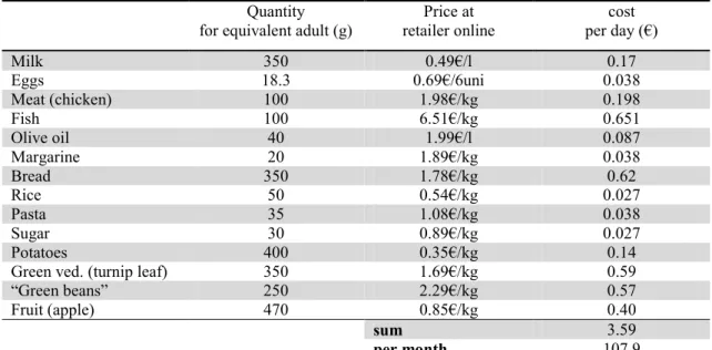
Table 1 shows the goods included in bf: quantities, price per quantity and total daily cost. [6]
Quantity for equivalent adult (g)
Price at retailer online
cost per day (€)
Milk 350 0.49€/l 0.17
Eggs 18.3 0.69€/6uni 0.038
Meat (chicken) 100 1.98€/kg 0.198
Fish 100 6.51€/kg 0.651
Olive oil 40 1.99€/l 0.087
Margarine 20 1.89€/kg 0.038
Bread 350 1.78€/kg 0.62
Rice 50 0.54€/kg 0.027
Pasta 35 1.08€/kg 0.038
Sugar 30 0.89€/kg 0.027
Potatoes 400 0.35€/kg 0.14
Green ved. (turnip leaf) 350 1.69€/kg 0.59
“Green beans” 250 2.29€/kg 0.57
Fruit (apple) 470 0.85€/kg 0.40
sum 3.59
per month 107.9
The final yearly expenditure in minimum food bundle was 1216,34€.
Based on bf we calculated several poverty lines. First, we calculated poverty lines with the Orshansky method using the average share of food spending on total spending of the whole sample.
We tried to define, afterwards, poverty lines using information about the population that is more likely to be poor (hence, not using features of the whole population). For this purpose we followed Ravallion’s (1998) [15] method of establishing an upper and a lower bound for the basic non-food spending and, hence, for the poverty lines. The author supports that one reasonable upper bound is the average total expenditure of the population whose food expenditure is (approximately) equal to the survival food bundle
(bf). To build the lower bound the author argued that the non-food expenditure of the people whose total spending was near bf should be a good proxy for the minimum non-food expenditure required by society to live in it. He proposed then that the minimum poverty line should be bf plus the average of non-food spending of those whose total spending was bf.
Based on these two criteria we constructed eight different poverty lines following three different approaches. The first approach was just to apply the Orshansky model using the share of food spending of the population that was in a neighborhood of bf (instead of using the whole population). We used two intervals: one of 10% and other of 20%. We label these lines “restricted Orshansky” lines. To get the upper bound we calculated the average Engel coefficient (share of food spending on total spending) of the people whose expenditure in food was within the specified interval centered in bf. We input this average share of food spending in the Orshansky formula to obtain the upper poverty line. In order to get the lower bound we calculated the Engel coefficient considering those people whose total expenditure was in a neighborhood of bf.
expenditure for food and still people waste money in non-food goods this expenditure could be a good proxy to that devoted to basic non-food goods.
The last approach consisted in running a regression to capture the average share of food-spending of people as a function of the relative distance of total food-spending to bf. The model used was
Where stands for the share or food spending on total spending, is adjusted total spending, d are demographic variables (we used number of elderly, number of children, proportion of women to men in the household and number of employed people) and , , and are parameters to be estimated; In the expression above, for (people on the poverty line) the resulting share would only differ due to demographic variables.. The upper bound for the poverty line is calculated as bf/ *, where * is found implicitly as . The lower bound is given by 2bf – f(bf)=(2- ) bf .10
After defining the different poverty lines we calculated the correspondent aggregation measures to quantify the dimension of poverty in Portugal. We did not pursue with the analysis of the results of the last approach because they were unsatisfactory, as explained below.
Finally, we ran some probit models in order to check the relationship that might exist between some features that the literature, mainly from sociology, points to characterize
the poorer of the society:11 the number of people in the household, living in urban centers or not, couples with no children, couples with one or two children, couples with more than three children, families where there are only elderly, adults that live lone, elderly living alone, mono-parental families, women living alone, elder women living alone, mono-parental families constituted by a female adult, number of workers, share of medical expenditure, expenditure in clothing, expenditure with education and existence of heating devices at home.
All the calculations were done in a per capita basis that took into account the economies of scale that may arise from cohabiting with other people. We used the OECD-Modified equivalence scale that is the one used by the EUROSTAT: this attaches weight 1 to the household’s representative, each of the other adults weights 0,5 and each child weights 0,3. From this point on we are going to refer to this expenditure per capita as adjusted expenditure.
V. Data
The data used in this article is from the 2005 Household Budget Survey (Inquerito as
Despesas da Familias) produced by the Portuguese Statistical Agency, INE.12 It has
been computed between 2005 and 2006 and it has information about the annual expenditure of 28359 individuals divided in 10403 households living in Portugal (Mainland and Autonomous Regions). The database has information about expenditure in more than 300 items as well as on facilities and an assessment of the durable goods that each family disposes of. The chosen individuals live all in domestic private households. The data was collected by direct questioning: accompanying each
11 For the choice of the variables we followed Capucha (2005) [3]
household during two weeks and registering every type of revenues and expenses they have.13
To develop the methodology explained above we used the following items: total expenditure, food expenditure, expenditure in restaurants, canteens and cafeterias, medical expenditure, clothing expenditure, expenditure in education, presence at home of utilities and heating. We used also the demographic characteristics described in the dataset.
The distribution of adjusted total expenditure can be seen in Appendix I.
VI. Results
VI.1 The Orshansky’s poverty line Table 2
Without restaurants With restaurants
Value of the poverty line (€/year) 6401.8 4261.29
HCR 38.9% 16,76%
In Table 2 we can see a comparison between the poverty line constructed with the Orshansky method (with the average share for the whole sample) for two different situations: in the first case we considered the expenditure in food being solely the expenditure in alimentary consumable goods; in the second case we included on food expenditure the spending on restaurants bars and canteens. As it can be seen results differ immensely: 1) not including the expenditure in food sellers might disregard the fact that most people do not have time or capacity to have lunch at home or bring their own lunch to work and this physical constraint will condition the share of total
expenditure devoted to nourishment; 2) at the same time, expenditure in restaurants can be seen as a luxury good, that should not count for basic needs. This would suggest that the first line is overestimated (too high) and the second might be too low. Even so, we chose as a benchmark to include spending in food selling establishments on food spending, as we believe that its effect should prevail towards the second argument outlined.
VI.2 Absolute Poverty lines and measurement
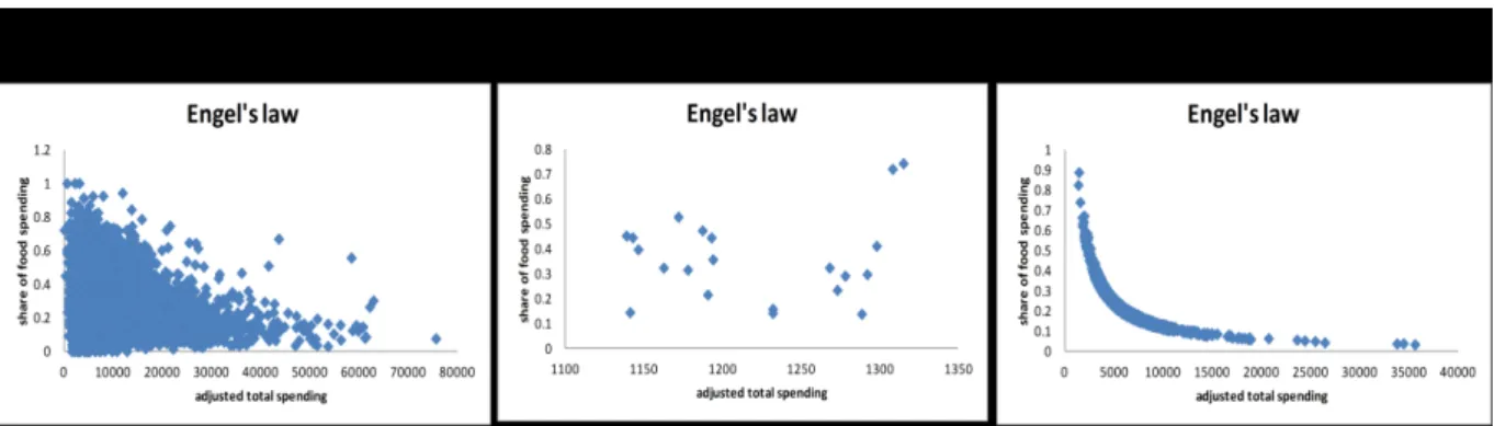
In order to have a feeling of how the variables of study behaved we first plotted the share of food spending with the adjusted total expenditure to see if our data respected the empirical Engel’s law (that states that these variables have a negative relationship). We performed the analysis: to (a) the whole population; (b) the population whose total spending is in a neighborhood of 20% around the food survival needs expenditure bf; (c) the population whose actual food spending is in a neighborhood of 20% around the food survival needs expenditure bf.
Figure 1: relationship between the Engel’s coefficient and the adjusted total spending.
between the variables for the whole population, in general terms, even if it is not perfect. For the lower income families (b) no relationship seems to exist.
In table 3 we show the poverty measures in terms of number of households for each line presented.14 The first row, PL, contains the value of each poverty line and the second row refers to the average share of food spending of the intervals considered. The last row presents the number of households within the intervals used to compute the poverty lines.
Table 3
restricted Orshansky Ravallion 1998
10% 20% NP
upper lower upper lower upper lower
P L 4789.44 3808.42 4885.35 3382.79 5965.34 2037.29
average share
food spending 0.253 0.32 0.249 0.36 0.25 0.32
HC 2294 1298 2406 940 3562 178
HCR (%) 22.05 12.48 23.13 9.04 34.24 1.71
PGR (%) 3.15 1.31 3.38 0.81 6.77 0.09
IGR (%) 27.18 25.1 27.33 24.13 30.26 23.21
FGT2 (%) 2.44 1.21 2.58 0.83 4.48 0.15
Ner households 450 10 907 20 907 20
From the analysis of the table we can see that the upper bounds of the restricted Orshansky method are quite similar. This is not surprising as the two intervals are not independent (the 10% is obviously inside the 20% one). Notwithstanding, it is worth to note the sensitiveness of the method to the approximation considered towards the shares: we can see that a decimal difference in the shares yields a difference between the lines of about 500€ for the lower bound. This difference is due to a bigger average share of food spending of the widest interval. This just means that when getting a larger
number of people, those observations that are in the extremes of the interval have a bigger average share than those in the centre (as can be seen in figure 1 (b)).
When comparing those lines with the non-parametric boundaries proposed by Ravallion we see that the thresholds for the latter are much apart from each other than the former. This can be partly explained by the wide disparity between choices of individuals regarding food and non-food goods making the average share of food spending less representative of the behavior of the population towards spending on basic needs (as it could be seen in figure 1 (b)). Further, we must be aware that our model expects everybody to have a healthy diet which is a strong assumption (experience tells us that one’s diet is very linked with many other features apart from income such as level of literacy, social groups in which is inserted). The two methods give results with a difference of more than 1000€ per year, which is not negligible as it represents almost 50% of the lower poverty threshold. When taking the expenditure in restaurants and cafeterias out of the adjusted food spending, these divergences become wider.
Table 4
Sensititvity analysis of bf
(a)
P L Restricted Orshansky Ravallion 1998
10% 20% NP
upper lower upper lower upper lower
bf 4789.44 3808.42 4885.35 3382.79 5965.34 2037.29
bf 5% lower 5084.46 3104.77 5244.9 3279.89 5525.94 1899.82
bf 5% upper 5137.2 3371.84 5044.93 3442.43 6369.14 2102.86
(b)
av. Share Restricted Orshansky Ravallion 1998
10% 20% NP
upper lower upper lower upper lower
bf 0.25 0.32 0.25 0.36 0.25 0.32
bf 5% lower 0.23 0.37 0.22 0.35 0.23 0.36
bf 5% upper 0.25 0.38 0.25 0.37 0.25 0.36
(c)
HCR Restricted Orshansky Ravallion 1998
10% 20% NP
upper lower upper lower upper lower
bf 22.05 12.48 23.13 9.04 34.24 1.71
bf 5% lower 24.98 7.03 26.71 8.25 29.71 1.31
bf 5% upper 25.65 9.01 24.63 9.45 38.63 1.89
Regarding the parametric approach proposed by Ravallion, we present below the results of the regressions.
Table 5
whole sample half sample
coefficient p-value coefficient p-value
α 0.4997 0 0.636 0
β1 -0.0326 0.052 -0.1106 0.004
β2 -0.00379 0.055 0.00698 0.198
R2 0.128 0.1398
Upper lower upper lower
PL 2570.46 1824.88 2133.94 1659.09
When running the regression with the whole sample, we obtained that all the coefficients were statistically significant at 1%. Even so, we got boundaries that were not in line with the ones found by the other methods (in fact too low). To test if we got more credible results considering only the half of the sample that is poorer (below the median adjusted total expenditure) we ran the regression again and we got worse results: β2 became not significant and the poverty thresholds were even lower. Hence, we decided to drop this method and we did not pursue with further considerations about it.
VI.3 Poor’s characteristics
To establish some relationships between the probability of being poor and the characteristics of this group, we ran probit models. For the choice of the variables, we selected some features pointed by Capucha (2004) [4] as being key features for describing the poor.
We report below the marginal effects of each variable on the probability of being poor. The level of significance is signed with * for 10% significance, ** for 5%, *** for 1%. Table 6:
(a) lower poverty lines
variable 10% 20% Non parametric
constant -1,835*** -2,0024*** -2,5171***
Household’s dimension 0,0545*** 0,04025*** 0,1021***
Urban area -0,03821*** -0,03251*** -0,01235***
Number of workers in the household
-0,06083*** -0,0461*** -0,0131***
Mono-parental families 0,0481 0,6537 -0,1308
Families with only elderly
0,06304*** 0,05208*** 0,00768
Couple with no kids (non elder)
0,02166** 0,01635* -0,000129
Couple with more than 2 children
-0,01021 -0,02296 -0,0174*
Alone pensioners 0,12826*** 0,0406834*** 0,00765
Adults (non elder) alone
0,0948*** 0,08606*** 0,028986***
Other types of families 0,07374*** 0,05736*** 0,01767***
Mono-parental families with woman
-0,00368 -0,03145 0,14203
Elderly alone women 0,0296 0,0427** 0,01928*
Women (non elder) living alone
0,00872 0,01518 -0,010839
Share of food spending 0,4635*** 0,34721*** 0,0850***
Share of restaurant spending
-0,0523*** -0,02794* -0.003246
Share of medical
expenditure
-0,0866*** -0,08623*** -0,0285***
Share Clothing
expenditure
-0,2206*** -0,15003*** -0,1136***
Share of Primary and kindergarten education exp.
-0,1239 -0,01042 _
Share lower secondary education exp.
-0,823** -3,9396 _
Share of Higher
education exp.
-0,3708*** -0,6244*** _
Share of other types of education exp.
-0,74216* -0,37808 _
Heating -0,0876*** -0,06739*** -0,01789***
(b) Upper poverty lines
Variable 10% 20% Non parametric
Constant -1,4139*** -1,3952*** -1,0339***
Household’s dimension 0,0726*** 0,07455*** 0,08729***
Urban area -0,0753*** -0,08069*** -0,10223***
Number of workers in the household
-0,08086*** -0,0804*** -0,08433***
Mono-parental families 0,03582 0,02757 0,07158
Families with only elderly
0,1008*** 0,09895*** 0,1271***
Couple with no kids (non elder)
0,01739 0,01695 0,0093
Couple with more than 2 children
-0,00985 -0,0045 0,00704
Alone pensioners 0,1553*** 0,16084*** 0,21253***
Adults (non elder) alone
0,13435*** 0,14725*** 0.12886***
Other types of families 0,10288*** 0,10053*** 0,120098***
Mono-parental families with woman
0,0145 0,03388 -0,00631
Elderly alone women 0,05681** 0,06356** 0,06150*
Women (non elder) living alone
-0,01621 -0,03063 -0,02668
Share of food spending 0,76572*** 0,7998*** 1,0371***
Share of restaurant spending
-0,02872 -0,03833* -0,03938*
Share of medical
expenditure
-0,06732** -0,06245** -0,09954***
Share Clothing
expenditure
-0,33992*** -0,35209*** -0,3961***
Share of Primary and kindergarten education exp.
-0,23985 -0,2907* -0,61001***
Share lower secondary education exp.
-0,75226*** -0,81137*** -0,8409***
Share of Higher
education exp.
-0,67224*** -0,74867*** -0,9763***
Share of other types of education exp.
-0,771715* -0,63887* -0,79001**
Heating -0,1216*** -0,1197*** -0,13932***
Pseudo-R2 0,1939 0,1934 0,1837
We can see that the variables that are persistently very significant and have the same sign across all the regressions are: the dimension of the household, the share of food spending on total spending that seem to have a positive relationship with the probability of being poor;15 the number of workers in the household, the share of expenditure in medical services, in clothing, on higher education, living in urban areas and the fact that
the households have some heating system at home that seem to be negatively correlated with the dependent variables. People living alone, pensioners or not, seem to be poorer than couples with one or two children (the control dummy variable). In addition there is some evidence that old women living alone are more likely to be poor than alone man. This might be partly explained by the fact that: 1) women tend to live more years diminishing the disposable private savings to spend per period of time; and 2) have a lower expected income along life relative to men.16
People tend to live in the house of their parents until a certain age, normally when they become financially independent. Besides that, when people retire, they often go to their children’s houses because they do not earn that much to sustain a house or just because they are no longer able to live alone. This makes us expect that bigger households have also bigger concentrations of people whose contribution to the household’s income is small. This is in line with the sign of the correlation we got for the number of people in the household. A similar reasoning can be applied in order to explain the effect found for the number of workers: the higher the number of workers, the higher the household’s income, the lower is the probability of being poor.
The positive coefficient of the share of food spending on total spending suggests that poorer people spend relatively more in food in terms of the overall spending than richer people. As there are minimum food requirements to stay alive people with lower income have to spend relatively more in food than wealthier people leading to a strongly positive correlation between the share of food spending and poverty patterns. The effect of the shares of the other expenditure might be explained by a similar
16See Cabral Vieira,J, A. Cardoso, A. R., Portela, M., (2003) “Gender segregation and the wage gap in Portugal: an analysis at the
argument: poor people have to spend a larger proportion of their total consumption in food and so a relatively lower proportion goes to non-food expenditure; moreover, the larger the disposable income the larger might be the share of consumption on non basic needs.
The presence of a heating system at home revealed to be negatively correlated with the probability of being poor. It is reasonable to assume that poorer people invest less in heating devices. Having access to heat can be considered a basic need and yet our model suggests that poorer people satisfy less this need than richer ones.
At last, in our work we could verify that, just as it occurred in the 80’s as stated by Costa 1992 [6], in the year 2005 people living in the rural and semi-rural areas were more likely to live in poverty than people living in urban areas.
VII. Conclusions
We studied poverty in Portugal from an absolute/normative approach. We established minimum standards of nourishment and measured poverty with different poverty lines. Building on Ravallion (1998) we established upper and lower bounds for poverty lines that respected two criteria for defining who was near poverty. We tried to quantify the effects of some features that are persistently claimed to be related with poverty.
relative approach basis. This fact points out that the calculation of poverty measures with the criterion used by the Eurostat reaches results that are consistent with a basic needs criterion for Portugal, in 2005.
Howbeit, we should not ignore that our results give a wide interval of possible thresholds. This dispersion could be partly explained, though, noting that people closer to the lower bound criterion are more likely to benefit from public provision of goods and services programs. This fact may influence both the share of food spending and the expenditure in non-food needs: the first item might be lower than the real value for the household, implying an upward bias of the lines constructed by the Orshansky method; the second item must be lower as well than the real use of non-food basic needs leading to a downward bias of the line constructed with the non-parametric method. This observation suggests that the real interval between the lower and the higher boundary should be smaller than the one we got in our calculations.
References:
[1] Alves, Nuno, 2009, “Novos factos sobre a pobreza em Portugal” Boletim económico
do Banco de Portugal – Primavera 2009, pp. 125-154.
[2] Atkinson, Anthony, 1991, “Comparing Poverty Rates Internationally: Lessons from Recent Studies in Developed Countries.” World Bank Review vol. 5, n.1, pp. 3-21. [3] Cabral Vieira, J. A., Cardoso, A. R., Portela, M., (2003) “Gender segregation and the wage gap in Portugal: an analysis at the establishment level”, Journal of Economic
Innequality, volume 3, number 2, pp. 145-168.
[4] Capucha, Luis, 2005, Desafios da pobreza, Celta, Oeiras.
[5] Citro, Constance and Michael, Robert, 1995, Measuring Poverty: a New Approach. National Academy Press, Washington DC
[6] Costa, A. B. et al, 2008, “Um olhar sobre a pobreza”, Gradiva.
[7] Costa, A. B., 1992 The Paradox of Poverty - Portugal 1980.1989. University of Bath.
[8] Costa, A. B. et al, 1985, “A Pobreza em Portugal”, Caritas Portuguesa.
[9]Feres, J. C., Mancero, X., 2001 “Enfoques para la medicion de la pobreza. Breve revision de la literatura”, CEPAL
[10] Feres, J. C., Mancero, X, 1998, “Notas sobre la medición de la pobreza según el método del ingreso”, Revista de la Cepal , n. 61, pp. 119-133.
[11] Foster, J., Greer, J. and Thorbecke, E., 1984, “A class of Decomposable Poverty Measures”, Econometrica, Vol. 52, ner
3.
[12] Forster, Michael F., 1994, “Measurement of low incomes and poverty in a perspective of international comparisons”, Working paper, OECD.
[13] Hagenaars, Aldi and Van Praag, Bernard, 1985, “A Synthesis of Poverty Line Definitions”. Review of Income and Health, vol. 31, n.2, pp 139-154.
[14] Melo, Ana Barbosa de, 2009 “Is help really helping?”, Work Project, FEUNL. [15] OECD, 2005, “Combating Poverty and Exclusion through Work”, Policy brief,
OECD.
[16] Orshansky, Mollie, 1963, “Children of the poor”, Social Security Bulletin vol 26, n.7, pp.3-13.
[17] PNUD, 1997, Informe sobre Desarrollo Humano, Oxford University Press, New York. 2, p. 122.
[18] Ravallion, Martin, 2010, “Poverty lines around the world”, Working paper World Bank.
[19] Ravallion, Martin and Loshkin, Michael, 2006, “Testing Poverty Lines”, Review of
Income and Wealth 52(3): 399-421.
0
0 20000 40000 60000 80000
adjusted total spending
[21] Ray, Debrah, 1998, “Chapter 8: Poverty and Undernutrition” in Development
Economics, pp 249-294, Princeton University Press
[22] Rodrigues, C. F., 1999, “Income Distribution and Poverty in Portugal [1994/95]”, CISEP, Working Paper ISEG, D36, I32.
[23] Rowtree, Seebolm, 1899, Poverty: a Study of Town Life. Macmillan, London. [24] Sen, Amartya, 1983, “Poor, relatively speaking”, Oxford Economic Papers 35, pp. 153-159.
[25] Spicker, Paul, 2007, “Definitions of poverty: twelve clusters of meaning”. In Gordon, David, Leguizamon, Sonia Alvarez and Spicker, Paul (eds), Poverty: an
international glossary. Zed Books
[26] Streeten, Paul, 1989, “Poverty: concepts and measurement”, Boston University, Institute for Economic Development Discussion Paper N.6.
[27] Townsend, Peter, 1979a, Poverty in the United Kingdom, London, Allen Lane and Penguin Books.
VIII. Appendix:
VIII.1 Appendix I