Electrical Power and Energy Systems

Robust feeder reconfiguration in radial distribution networks

Carlos Henrique Nogueira de Resende Barbosa

_{, Marcus Henrique Soares Mendes}

_,

João Antônio de Vasconcelos

a_{Federal University of Ouro Preto, Department of Electrical Engineering, Rua 37, no. 115, Loanda, CEP: 35931-026 João Monlevade, MG, Brazil} b_{Federal University of Viçosa, Campus Florestal, Rodovia LMG 818, km 6, CEP: 35690-000 Florestal, MG, Brazil}

c_{Federal University of Minas Gerais, Graduate Program in Electrical Engineering, Av. Antônio Carlos, 6627 – Pampulha, CEP: 31270-901 Belo Horizonte, MG, Brazil}

a r t i c l e

i n f o

Article history: Received 21 May 2012

Received in revised form 25 July 2013 Accepted 21 August 2013

Keywords: Interval analysis Feeder reconfiguration Multi-objective optimization Radial distribution networks

a b s t r a c t

Distribution feeder reconfiguration has been an active field of research for many years. Some recent the-oretical studies have highlighted the importance of smart reconfiguration for the operating conditions of such radial networks. In general, this problem has been tackled using a multi-objective formulation with simplified assumptions, in which the uncertainties related to network components have been neglected by both mathematical models and solution techniques. These simplifications guide searches to apparent optima that may not perform optimally under realistic conditions. To circumvent this problem, we pro-pose a method capable of performing interval computations and consider seasonal variability in load demands to identify robust configurations, which are those that have the best performance in the worst case scenario. Our proposal, named the Interval Multi-objective Evolutionary Algorithm for Distribution Feeder Reconfiguration (IMOEA-DFR), uses interval analysis to perform configuration assessment by con-sidering the uncertainties in the power demanded by customers. Simulations performed in three cases on a 70-busbar system demonstrated the effectiveness of the IMOEA-DFR, which obtained robust configura-tions that are capable to keep such system working under significant load variaconfigura-tions. Moreover, our approach achieved stable configurations that remained feasible over long periods of time not requiring additional reconfigurations. Our results reinforce the need to include load uncertainties when analyzing DFR under realistic conditions.

Ó2013 Elsevier Ltd. All rights reserved.

1. Introduction

Reconfiguration of radial distribution networks is a viable op-tion for ensuring optimal or nearly optimal operaop-tion in the pres-ence of several constraints and variable power demand[7,16,18–

22,35]. From a theoretical perspective, distribution networks can

always be reconfigured whenever imminent loading variations are detected. Even though optimization procedures may reveal improvements on power losses, voltage flatness or load balancing related to a given distribution network, it is important to realize that maneuvers performed by power utilities are still costly, lack appropriate equipment [35], and hence, they are unusual when such systems are operating normally. Although feeder reconfigura-tion seems to be very attractive to optimize the system’s operating conditions, supervisory centers adopt a conservative strategy to avoid switching maneuvers as much as possible. This behavior can be justified by the low level of network automation and the

imminent risks due to interference with protective devices, which may cause unexpected overloads or interruptions in the power supply. From the practical standpoint, maneuvers are the preferred procedure for solving critical or abnormal situations, but rarely for performance optimization.

Under normal conditions, seasonal variations in power demand require utility companies to rely on demand estimation models to properly meet demand within safety margins and quality indexes

[4,6,16]. In these models, consumers are statistically classified

according to their average demand[6]. Loading forecasts contain inherent errors because these approaches are based entirely on esti-mations. In addition, renewable energy has given its contribution to the power demand variation on load buses which originally acted as strict consumers. Its importance to the distribution systems may no longer to be neglected once the growing proportion of power gener-ated by alternative means is intended to fill the gap between peak load demands and energy availability at regional extent[7].

A naive approach would treat network parameters as exact or definite values, and this approach could mistakenly assess a given configuration as optimal, adequate or fair to uncertainty-free envi-ronments. However, these configurations may be insufficient or even impracticable in the presence of power demand uncertainty.

0142-0615/$ - see front matterÓ2013 Elsevier Ltd. All rights reserved. http://dx.doi.org/10.1016/j.ijepes.2013.08.015

⇑ Corresponding author at: Federal University of Ouro Preto, Department of Electrical Engineering, Rua 37, no. 115, Loanda, CEP: 35931-026 João Monlevade, MG, Brazil. Tel.: +55 31 34093426; fax: +55 31 34095480.

E-mail addresses:carloshnrb@gmail.comC.H.N. de Resende Barbosa),marcus. mendes@ufv.br(M.H.S. Mendes),jvasconcelos@ufmg.br(J.A. de Vasconcelos).

Contents lists available atScienceDirect

Electrical Power and Energy Systems

Hence, it is important to obtain robust solutions. In our approach, robust solutions are those solutions that are less susceptible to uncertainties and they are able to maintain a system normally operating even in the worst case scenario. In this work, we re-stricted uncertainties to PQ loads, because they are among the most relevant factors in feeder reconfiguration decisions, mainly if we consider power generation in those buses [12,32–34]. Be-cause feeder reconfiguration depends on some power flow method [2], uncertainties must be accounted for using a mathematical model capable of reflecting all immediate effects on the power flow

[11,12,32,33].

Feeder reconfiguration is considered a combinatorial problem with an irregular search space[26,31]and is generally formulated as a restricted multi-objective problem. The radiality constraint and the discrete nature of the switches prevent the use of classical techniques to solve feeder reconfiguration[2,18,19,23,25,27]. An evolutionary stochastic approach was chosen because this ap-proach is relatively unaffected by the nature of the problem. As previously mentioned, an efficient solution set in a deterministic environment can be partially or totally impaired in a perturbed environment, which moves these solutions away from the Pareto frontier[14]. Thus, a conventional approach will probably fail to identify an efficient solution set to the feeder reconfiguration prob-lem. Therefore, we present a proper implementation, in which a Multi-Objective Evolutionary Algorithm (MOEA) based on NSGA-II[13]was coupled to an interval version of the Backward/Forward Sweep Method (BFSM). This novel hybrid approach, which we call Interval Multi-objective Evolutionary Algorithm for Distribution Feeder Reconfiguration (IMOEA-DFR), is a robust method of solving

reconfiguration problems. To our knowledge, there is no study encompassing this specific issue yet. The objectives of this work are (i) to provide a new strategy that properly addresses load uncertainties in DFR optimization (see Section5), (ii) to demon-strate the fragility of optimal solutions found by conventional ap-proaches in uncertain real-world environments (see case 2 in Section6), and (iii) to discuss how robust solutions can replace pseudo-optimal solutions to ensure reasonable and satisfactory network operating conditions in the worst case scenario (see case 3 in Section6).

This paper is organized as follows. In Section2, related works are cited, and their primary contributions are highlighted. The for-mulation of the DFR problem is presented in Section3. In Section4, the background of interval analysis is addressed, and the robust version of the DFR problem is defined. The implemented algorithm and related issues are described in Section5. Finally, a discussion about computational experiments is presented in Section6, and concluding remarks are given in Section7.

2. Related works

The feeder reconfiguration has been treated as a typical uncer-tainty-free problem in many papers[2,3,7–10,15,25,26,29]. From a classical perspective, these approaches are satisfactory, and their solution sets are valid whenever uncertainties are negligible. How-ever, these solutions are not as reliable as they seem[5]. It has been shown that electrical power systems are subjected to many sources of uncertainty such as power (load) demand[16,20–22], distributed generation[21,22], and electrical parameters[5,6,35].

Nomenclature

NB bus set size

NL distribution line set size

Ns number of sources

Nw total number of switches

Nf number of objective functions

Nv number of uncertainty parameters

x binary vector containing all the switches statuses xc _{cth configuration}

Bs set of all buses supplied by sources Zi impedance of theith distribution line

Ii current flow in theith distribution line

Imax

i ampacity (maximum current) of theith distribution line

Vk actual voltage at busk

Vnom

k nominal or normalized (p.u.) voltage at busk

||X|| size of a given setX |v| modulus of the variable

v

a+ _{upper bound of an interval vector}

P set of uncertainties X set of decision variables p vector of uncertainty parameters f vector of objective functions g vector of inequality constraints h vector of equality constraints

Due to the importance of these uncertainties regardless their nat-ure in the reconfiguration problem, seen in Section1, it is notewor-thy to mention the works that have addressed power flow methods under uncertain environments. Some authors have proposed ver-sions of power flow analysis to cope with uncertainties

[6,12,32,34,35]. Load variations were modeled for network

plan-ning purposes by Chaturvedi et al.[6]and later by Borges and Mar-tins[4]. In[6], a proposal was devised based on interval arithmetic approach that represents loads through Gaussian probability den-sity functions. Vaccaro presented an alternative to the sampling-based technique applied to radial power flow analysis supported by interval mathematics[32] or affine arithmetic [33]. He was the first to introduce an affine arithmetic approach[33] to find the distribution network’s operating point, while considering vari-ation in load and genervari-ation levels. His proposals were intended to tighten variables’ domains without losing valid solutions. Still, fewer loadflow methods are able to deal with uncertainties in ra-dial networks[4,6,11,27]. Das used an interval analysis technique to perform power flow analysis in unbalanced[12]and balanced [11] three-phase radial distribution systems while considering load and feeder parameters uncertainties. Zhang et al. [35] pro-posed a method called Reliability-Oriented Reconfiguration (ROR) which employed interval analysis to quantify the impact of uncertain data on system parameters and to maximize the

possi-bility of reliapossi-bility improvement and/or loss reduction achieved through reconfiguration.

As previously detailed, many researchers have studied strate-gies for coping with uncertainties in power flow analysis to tackle reconfiguration problem in a broader manner. This work goes far-ther and deals suitably with the robust DFR problem focusing on network operation. Our IMOEA-DFR approach applies interval analysis not only to power flow algorithms, but also to non-domi-nance assessments among solutions in terms of the worst case per-formance. Therefore, the primary contribution of this manuscript is to provide an effective method of finding robust configurations that guarantee the operating conditions of distribution feeders un-der uncertain loading.

3. Problem formulation

Our mathematical formulation is derived from[3]. The on/off statuses of allNwmaneuverable switches were used as optimiza-tion variables and coded into a binary vectorx(x= [x1,. . .,xi,. . .,

xNw]) whose ith element indicates whether the corresponding switch is open (xi= 0) or closed (xi= 1). Each distribution line has its own switch (NL=Nw= ||x||). As in [15], four objectives were assumed in this formulation: Power Losses (PL), Current Loading

(a)

(b)

(c)

Index (CLI), Voltage Deviation Index (VDI), and Number of Switch-ing Maneuver (NS). PL can be described as follows:

PL¼ X

Nw

i¼1

xiReðZiÞ jIij2 !

; ð1Þ

whereRe(Zi) is the real component of theith line impedance andjIij corresponds to the magnitude of the current flowing through theith line. The second objective is mathematically represented as:

CLI¼ 1

Nw XNw

i¼1

xiIi=Imaxi !

: ð2Þ

The third objective involves minimal voltage deviation from the nominal values at allNBbuses in the system. To implement this cri-terion, the index proposed by Sahoo et al.[25], which requires sim-ple computations, was modified by Huang and represented as[15]:

VDI¼ 1

NB XNB

k¼1

xC

i;k VkVnomK

!

; xC

i;k2W; ð3Þ

whereWdenotes a set of all closed switches andxC

i;kindicates that switchiis closed to connect buskto a power node in configuration

c. The fourth objective considers the number of switching maneu-vers, which must be kept as small as possible due to operational costs and network management considerations. This objective is calculated using the Manhattan distance:

NS¼X

Nw

i¼1

xc ix0i

; ð4Þ

wherexc

i andx0i denotes each set of corresponding switches in the candidate and previous configurations, respectively. The distance between any corresponding switch equals xc

ix0i

. Additional, restrictions were admitted. Radiality must be ensured using the fol-lowing relations:

NBNs¼ kWk ¼ XNw

i¼1

xc

i; ð5:aÞ

XNs

s¼1

bs_k¼1;

8

xc

i;k6xci1;k1jxci1;k1¼1()Bs:¼Bs[bsk1

8

8

ð5:cÞ

The condition in Eq.(5.a)holds for anycradial configuration or set of configurations, but it does not guarantee radiality by itself. In

Eq.(5.b),bskis a binary variable that takes the value one (zero) to

indicate that buskis fed (not fed) by sources. This statement is complemented by Eq.(5.c), wherein the status of theith switch

xc i;k

, which delivers power to thekth bus, depends on the status

of an adjacent switch, xc i1;k1

, closer to the (temporary) common sources, which in turn delivers power to thek1th bus. All of the

NBbuses must be connected to available sources by a unique path to avoid loop or islanding. The following restriction ensures that the current in each line (or branch) does not exceed its ampacity:

jIij6Imaxi ; i2W: ð6Þ

The final restriction establishes that no valid solution may vio-late upper and lower limits of the bus voltages:

Vmin_k 6Vk6Vmaxk ; k¼1;. . .;NB: ð7Þ

The values ofVmin

k andV

max

k were assumed to be 0.9 p.u. and 1.05 p.u. on our simulations, respectively, according to the values defined in Baran’s work[2]. It is worthy to note that voltage restric-tion is complementary to Eq.(3)whose goal is to reduce as much as possible bus voltage variation.

3.1. Component modeling issues

Power can be re-routed through reconfiguration, i.e., opening and closing sectionalizing and tie switches. Reconfiguration is an effective way to operate distribution networks under load de-mands changes by redistributing currents through various lines to prevent or alleviate overloading in system equipment, reduce real power losses, improve the voltage profile and increase system stability. Feeders may serve a variety of different consumers who can be organized into classes such as residential, commercial, or industrial[16]. Each class has its own peak time, and their load behaviors affect the overall loading over the 24-h cycle. Depending on the chosen configuration and distribution of those classes, restrictions can be violated in some instances. In these cases, the system must be reconfigured in advance to avoid potential risks to system stability (e.g., equipment overloading or non-prescribed bus voltages).

an inherent degree of uncertainty. We incorporate uncertainties by assigning specified ranges to each bus. Loads can vary considerably throughout the day. Thus, the current configuration may be subop-timal or even invalid due to violations of some restrictions. These variations can be understood as perturbations to the system. In this work, a perturbation is characterized by well-defined uncertainty ranges on specific buses. To account for uncertainties, real and reactive power loads at the buses were treated as interval numbers.

4. Interval analysis

This section addresses the basic concepts and definitions of Interval Analysis (IA) required to understand how the proposed algorithm deals with intervals. More detailed information can be found in[17]. IA approaches use a range-based model that repre-sents a punctual number and its uncertainty. The model presented in this work uses interval numbers to indicate the spread of a numerical value. A real, closed and connected interval is defined as:

Definition 1. A closed interval [a] is a connected subset in R defined by

½a ¼ ½a_;aþ

:¼ fa2Rja6a6aþg; ð8Þ

where a _{and a}+ _{represent the lower and upper bounds of [a],} respectively. The set of all intervals defined by(8)represents the set of real intervalsðRÞ.

Definition 2. The multi-dimensional real interval½a 2Rn, denom-inated box or interval vector is given by

½a ¼ ½a1 ½a2 . . . ½an: ð9Þ

Definition 3. The lower bound a _{of [a] is given by} a_{¼ a}

1;a2;. . .;an T

. In the same way, the upper bound

aþ_{¼ a}þ

1;aþ2;. . .aþn T

.

Definition 4. The four classical operations of real arithmetic can be extended to intervals. For any such binary operator, denoted byH, perform the operation means computing

½a

H

H

Regarding the extreme bounds, each classical operation for non-empty closed interval is given by:

½a þ ½b ¼ ½a_þb

;aþ_þbþ

: ð11Þ

½a ½b ¼ ½a_bþ

;aþ_b

: ð12Þ

0 10 20 30 40 50 60 70

0 200 400 600 800 1000 1200 1400

R

eal

P

o

w

e

r D

e

m

a

n

d

(kW

)

Real Power Demand Ranges at Load Buses

Bus Numbering

0 10 20 30 40 50 60 70

0 200 400 600 800 1000 1200 1400

R

eacti

ve P

o

w

e

r D

e

m

a

n

d

(kV

A

r)

Reactive Power Demand Ranges at Load Buses

Bus Numbering

(a)

(b)

½a ½b ¼ ½minðsÞ;maxðsÞ; being

s¼ fa_b ;a_bþ

;aþ_b ;aþ_bþ

g: ð13Þ

½a=½b ¼ ½a ð1=½bÞ; Where

1=½b ¼/; if½b ¼ ½0;0: 1=½b ¼ ½1=bþ;1=b; if 0R½b:

1=½b ¼ ½1=bþ;1; ifb¼0^bþ>0:

1=½b ¼ ½1;1=b; if b<0^bþ¼0:

1=½b ¼ ½1;1; ifb<0^bþ>0:

ð14Þ

It is noteworthy that the interval addition, subtraction, multi-plication, and division operators operate on any two interval oper-ands to produce an interval result that contains all arithmetical combinations of the interval numbers describing the operands.

As shown in the next subsection, we represent the power de-mands on the PQ buses using interval numbers to guarantee that all uncertainties on the loads are taken into account. In terms of implementation, every real operation that uses interval variables is replaced by the respective interval operator in the power flow analysis algorithm. Therefore, the fundamental theorem of IA [17] guarantees that all obtained outputs are contained within the interval result.

IA includes an inherent pessimism related to the interval oper-ations, meaning that the output interval may be overestimated. For

instance, the real expressions f=x(1x) and g=xx2 _are equivalent in real arithmetic. However, assuming [x] = [0, 1], their interval counterparts lead to distinct results given thatf[x] = [0, 1] andg[x] = [1, 1]. Both results represent an enclosure of the correct output regarding the input interval. On the other hand, the former is narrower (is less pessimistic) than the latter. In general, this pes-simism arises as a result of multiple occurrences of the same var-iable. Mathematical reorganization of the expression can resolve this problem, but variable multiplicity may not always be avoidable.

4.1. Non-dominance analysis in an interval context

In this paper, we compute the worst case performance of each solution by considering the uncertainty parameters (uncertainty in the load demand on each PQ bus) using intervals. The worst case performance of a configuration is computed using:

fwcðx;pÞ ¼max

p2Pfiðx;pÞ; i¼ f1;. . .;Nfg: ð15Þ

In Fig. 1, three spaces representing the uncertainty, decision

variable, and objective are represented in two dimensions to illus-trate the procedure by which the objective functions are evaluated for each configuration inXby considering perturbations inP. Thus, a configuration is associated with a box in the objective space. The

0 10 20 30 40 50 60 70

0 200 400 600 800 1000 1200

Bus Numbering

Reactive Power Demand (kVAr)

Reactive Power Demand Ranges at Load Buses

0 10 20 30 40 50 60 70

0 200 400 600 800 1000 1200

Real Power Demand (kW)

Real Power Demand Ranges at Load Buses

Bus Numbering

(a)

(b)

worst case performance is represented by the black filled-in circle on the upper right corner of each box. According toDefinition 6, the dotted boxes are dominated by at least one of the other boxes.

Definition 5. Given that u and

v

v

v

v

Nf},ui6

v

v

Definition 6. The dominance operator is extended to interval com-putation as follows

½a ½b ()aþ_bþ

: ð16Þ

4.2. The robust formulation

The worst case Robust Multi-objective Optimization Problem (RMOP) can be seen as maximizing the effects of uncertainty on the objective functions, and subsequently minimizing all objective functions, as described in [30]. Mathematically, given that x2X#RNw_;p2P#RNpandfðx;pÞ:RNwRNp#RNfthe RMOP is defined by:

min

x2S maxp2P fðx;pÞ ¼ ff1ðx;pÞ;. . .;fNfðx;pÞg; ð17Þ

where the feasible space is given by:

0 10 20 30 40 50 60 70

0 200 400 600 800 1000 1200 1400

Bus Numbering

Real Power Demand (kW)

Real Power Demand Ranges at Load Buses

0 10 20 30 40 50 60 70

0 200 400 600 800 1000 1200 1400

Bus Numbering

Reactive Power Demand (kVAr)

Reactive Power Demand Ranges at Load Buses

(a)

(b)

Fig. 6.Ranges of the (a) real and (b) reactive power demands of the load buses in case 3.

Table 1

Optimal solutions to the 70-busbar system (the last two data columns consider 8% uncertainty for all loads).

Parameter Reference solution found in [15]

MOEA-DFR solution

Reference solution considering uncertainty effects

IMOEA-DFR solution

Real power loss (kW) 113.406 113.406 [96.5678, 134.125] [96.592, 134.1582]

Voltage deviation index 0.0129 0.0129 [0.011851, 0.013959] [0.011804,

0.013905]

Average current loading index 0.1860 0.1860 [0.17297, 0.20342] [0.17268, 0.20308]

Switching number 4 4 4 4

Overall minimal bus voltage (p.u.) 0.9288 0.9288 [0.92288, 0.93471] [0.92288, 0.93471]

Maximum current loading index 0.9203 0.9203 [0.84664, 0.99388] [0.84664, 0.99388]

Proposed solution (opened switches)

S:¼ fx2Xjgðx;pÞ60^hðx;pÞ ¼0

8

Solving(17)allows us to find a set of robust minimizers, which can be written as:

X

:¼ x::9xjmax

p2P fðx;pÞ maxp2P fðx

_;pÞ

8

Particularizing the RMOP to the DFR problem, we haveNf= 4 objective functions: f1= power losses, f2= current loading index,

f3= voltage deviation index, andf4= number of switching maneu-vers. In addition, there are three constraints:h1= involving radial-ity – formed by Eqs.5.a, 5.b, 5.c,g1ensuring current values less than ampacity for each line (or branch) – Eq.(6), andg2which is related to the upper and lower limits of bus voltages – Eq.(7). The values of f1,f2, f3, andg1, g2 are directly influenced by the uncertaintiespexisting in load demands of each PQ bus. Hence, for the first three objective functions and two inequality con-straints, intervals are obtained as output of the IMOEA-DFR. Since

f4is calculated by the number of switches to be maneuvered in or-der to change the initial configuration into the candidate solution, the influence of uncertainties is not straightly represented in this objective function. The constraint h1 considers the topology of the configuration. Consequently, power demand uncertainties do not have an immediate effect over configuration topology. In prac-tical terms,f4andh1can be represented by integers and, thus, they are handled as degenerated intervals in which lower and upper bounds assume the same value.

5. Implemented algorithm

As stated in Section1, DFR is a discrete combinatorial problem, and classical techniques are thus inappropriate for solving this optimization problem[18,19,23], which is reinforced by the radial-ity constraint. Many other techniques proposed in the literature are based on heuristic search strategies. In addition to being time-consuming, these techniques are restricted to network spec-ificities and do not guarantee an optimal solution. Evolutionary

algorithms are potentially capable of finding optimal or near-opti-mal solutions because they are not as limited as heuristics algo-rithms. Here, we propose an evolutionary algorithm based on NSGA-II[13]as the framework for finding non-dominated solu-tions. The fitness evaluation is computationally costly, and every new solution must be submitted to the iterative Backward/For-ward Sweep Method (BFSM), which employs the recursive sets of equations found in[9]. Both the P-Q decoupled method and the classical Newton–Raphson method are unsuited to solving distri-bution network power flow. For this reason, the BFSM method with power aggregation [1] was used to compute bus voltages and power losses.

The topological analysis, which generates and modifies configu-rations, is another costly task and demands a considerable fraction of the overall computing time. To assure the feasibility of all eval-uated individuals including those generated and those obtained from crossover and mutation operators, a Prim-like constructive heuristics is employed. A straightforward analogy can be made be-tween the distribution system and the graph theory. Buses and dis-tribution lines are equivalent to nodes and edges. Any disdis-tribution network can be represented as a graphG(N,A) that contains a set of nodes,N, and edges,A. We employ a constructive heuristic for two purposes: (i) to create random radial configurations, and (ii) to per-form crossover between two radial configurations. This method is simple and easy to implement, and solution diversity is guaranteed because every edge has the same probability of being chosen. More details about the crossover procedure based on a Prim-like heuris-tic are given in Algorithm 1.

Table 2

The best frontier found by MOEA-DFR or IMOEA-DFR in three scenarios: (i) original scenario described in[15], (ii) the perturbed scenario, and (iii) the interval scenario.

Switching number

Original scenario (40 solutions)

Perturbed scenario (65 solutions)

Interval scenario (75 solutions)

0 1a ₁a ₁a

2 1 11 3

4 4 (Huang solution included)

20b ₁₁b

6 15 22 30

8 19 11 30

a_{Initial solution.}

b _{Huang solution was discarded due to dominance criteria.}

Table 3

Performance comparison between Huang configuration and solution found by IMOEA-DFR. The best objective values are in italics.

Configuration Original scenario (nominal loads) Perturbed scenario (loads with uncertainty)

Real power loss (kW)

Voltage deviation index

Average current loading index

Overall minimal voltage (p.u.)

Maximum current loading index

Real power loss (kW)

Voltage deviation index

Average current loading index

Overall minimal voltage (p.u.)

Maximum current loading index

Huang solution[13] {13, 59, 70, 71, 74}

113.406 0.0129 0.1860 0.9288 0.9203 73.219 0.0169 0.1759 0.9582 0.9159

Identified solution by IMOEA-DFR {13, 20, 59, 65, 70}

107.962 0.0120 0.1872 0.9322 0.9203 55.902 0.0107 0.1752 0.9745 0.9159

6 10 12 16 18 22 24

0 50 100 150

Time (hours)

R

eal

P

o

w

er

L

o

ss (

kW

)

Daily Real Power Loss for Three Configurations

Conf. proposed by IA Huang's Configuration Original Configuration

Algorithm 1. Constructive heuristic adapted for crossover.

FUNCTION: Generation of two feasible configurations.

INPUT:C1=G(N,A1),C2=G(N,A2) andG(N,A) in which (A1,A2A)

OUTPUT:C0 1,C02 1 n 1

2 Whilen62

3 Define residual setR:¼An fA1[A2g

4 Initialize the following sets: active nodesO /, included nodesN0 _{/and included edgesA}0 _/.

5 Select one node

v

v

6 O f

v

v

v

u

e

e

8 Do

9 Choose nodeo(o

e

10 If$e|e= (o,p)

e

11 Else if$e|e= (o,p)

e

and go to line 14,

12 Else if$e|e= (o,p)

e

14 O p[O N0 _p[N0 _A0 _e[A0 _A

sel Aselne. Go to line 16.

15 O p[O N0 _p[N0 _A0 _e[A0 _{R Rne}

16 i 3n

17 UntilNnN0_–/ 18 C0

n GðN0;A

0 Þ 19 n n+ 1

20 End While

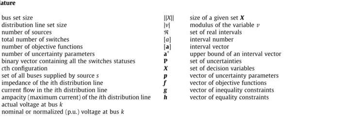
The purely constructive heuristic builds a configuration from an initial node. Subsequent nodes are added one by one, according to the available edges. If a chosen edge creates a loop, it is discarded, and it is replaced by another, chosen at random. This procedure terminates when all nodes are included. A semi-destructive heuris-tic is used to repair a configuration when the mutation operator is applied. This heuristic is able to detect loops as well as islanding. An open edge is closed to form a loop, and another edge belonging to this loop is opened. Although time-consuming, these two heu-ristics prevent useless evaluations in the proposed evolutionary algorithm and enable efficient exploration of the entire search space.Fig. 2(a and b) shows how new candidate solutions are ob-tained from genetic operators.

We initially implemented a non-interval algorithm, called the Multi-objective Evolutionary Algorithm for Distribution Feeder Reconfiguration (MOEA-DFR), to validate our evolutionary strategy by comparing its results with those achieved by the Enhanced Ge-netic Algorithm[15](see Section6, case 1). The MOEA-DFR is inca-pable of dealing with uncertainties and uses non-interval BFSM and the dominance criteria based onDefinition 5in Section4. Next, the MOEA-DFR was improved to include the ability to deal with the worst loading uncertainty case through the use of interval compu-tation, resulting in the IMOEA-DFR, which is illustrated inFig. 2(c). All real mathematical operations and variables in the BFSM were replaced by their interval operator and interval variable counter-parts, respectively. The algorithm only uses basic mathematical operations (addition, subtraction, multiplication and division) and two elementary functions (square root and exponentiation). In IMOEA-DFR, the non-dominance criteria are implemented according toDefinition 6in Section4.

6. Experimental results

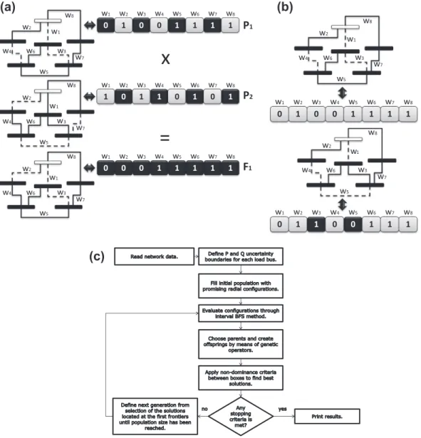
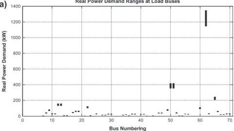
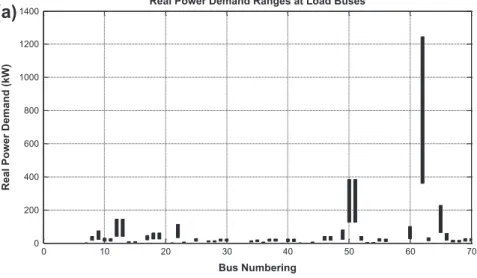
Experiments were performed with a known feeder that has al-ready been analyzed in the literature by Huang[15] and Chiang and Jumeau[8]. This feeder was originally presented in[1]and is redrawn inFig. 3for the sake of clarity and completeness. In this figure, the italic numbers denote the labels of the distribution lines, and buses are identified by the number positioned inside of them. The experiments were divided into cases 1, 2, and 3. Case 1 al-lows the original real and reactive power demands values in[1]to vary within a tolerance of 8%.Fig. 4(a and b) shows the ranges of each bus. Case 2 considers distinct perturbations to the load values on each bus.Fig. 5(a and b) shows the ranges of the load values of each bus. Case 3 uses the demand curves obtained in[28]to de-scribe seasonal variations in loads according to five profiles. These profiles were assigned to each load bus of the original test feeder in [1]according to the range of the value loads. Uncertainties were incorporated by assigning specified ranges to each bus by consid-ering the minimal and peak values (nominal values of the original test feeder) of each profile (Fig. 6(a and b)). It is noteworthy that the uncertainties in cases 2 and 3 are more significant than in case 1 and that they are related to considerable oscillations in the load demand.

Computational experiments were performed using Matlab ver-sion 7.10.0.499 (R2010a) and the INTLAB toolbox[24], running on a i3 Core CPU with 2.13 GHz and 4 GB of RAM memory, to evaluate the simulations involving interval analysis. The following evolu-tionary algorithm parameters were held fixed: population size (60), maximum number of generations (30), and probabilities of crossover (0.98) and mutation (0.05).

6.1. Case 1

InTable 1, the first and second data columns present the results

obtained in [15] and from the MOEA-DFR, respectively, for an uncertainty-free 70-busbar feeder problem. The two sets of results are in agreement, which validates the MOEA-DFR in the uncer-tainty-free case. The initial configuration was assumed to be the same as that used in[15]. It is important to note that even though the proposed formulation in[15]was multi-objective, the fitness assignment was performed by a weighted-sum of objectives, and the authors provided only a single solution rather than a Pareto frontier. The MOEA-DFR generates a frontier, and we have shown that the Huang solution is contained on the achieved frontier. The last two data columns inTable 1 show the ranges of each objective of the Huang solution and one solution pertaining to

the best frontier achieved using IMOEA-DFR, respectively, when uncertainties are included in the model. In this case, the two solu-tions are non-dominated by each other underDefinition 6 (Sec-tion 4). Therefore, given the uncertainties in case 1, both solutions can be properly adopted in real-world environments. In contrast to other methods, the IMOEA-DFR accounts for uncertain-ties in the modeling, and the robustness of the solutions is thus guaranteed. It is valuable to mention that the MOEA-DFR attained the Huang solution for ten distinct executions.

6.2. Case 2

Assuming the same uncertainty for all loads is naive because each bus generally has a distinct demand profile. Hence, in case 2, we assumed different levels of uncertainty for each load values.

Fig. 5presents the power demand range at each load bus. In case 2,

we worked with three scenarios: (i) the original scenario described in[15], (ii) a perturbed scenario in which the uncertainties lead the load values to the boundary opposite that they were in original scenario when considering the power demand range in Fig. 5, and (iii) the interval scenario represented by the ranges at each bus inFig. 5. Scenarios (i) and (ii) were solved by MOEA-DFR, while scenario (iii) was solved with the IMOEA-DFR. The frontiers ob-tained in the experiments in case 2 were built from ten distinct executions of the MOEA-DFR and IMOEA-DFR, whose parameters were adjusted to default values, as previously explained. The final frontier of each scenario was built by joining all non-dominated solutions belonging to the optimal frontier in each execution.

Ta-ble 2presents the distributions of the solutions found in each

sim-ulated scenario according to the number of switching operations. The MOEA-DFR found frontiers Froand Frp, which have 40 and 65 feasible solutions, respectively, to the simulated 70-busbar system in original and perturbed scenarios. The intersection between FrO and FrP contained only the initial solution because the fourth objective of the formulation requires that this solution remains on the final frontier of both sets (see Section3). Thus, we conclude that all solutions in FrOare unfeasible or suboptimal configurations in the perturbed scenario. To obtain configurations that are suit-able in all combinations of the original and perturbed scenarios, we use IMOEA-DFR to solve the interval scenario, which considers sufficiently large uncertainty margins to encompass the original and perturbed possibilities. IMOEA-DFR found frontier FrIwith 75 feasible solutions, of which fourteen solutions were shared with FrOand four solutions with FrP. As expected, only the initial solu-tion exists at the intersecsolu-tion between frontiers FrO, FrPand FrI. Table 5

Hypervolume values for the results found by IMOEA-DFR.

Case number Hypervolume metric for 10 runs Indicators

1 2 3 4 5 6 7 8 9 10 Mean Standard deviation

1 0.0355 0.0349 0.0349 0.0341 0.0348 0.0357 0.0353 0.0352 0.0351 0.0349 0.0351 0.0004 2 0.0214 0.0205 0.0212 0.0207 0.0195 0.0212 0.0212 0.0207 0.0209 0.0213 0.0208 0.0006 3 0.0351 0.0384 0.0379 0.0377 0.0351 0.0354 0.0350 0.0352 0.0379 0.0381 0.0366 0.0015

Table 6

IGD values for the results found by IMOEA-DFR.

Case number Inverse generational distance for 10 runs Indicators

1 2 3 4 5 6 7 8 9 10 Mean Standard deviation

It is worthwhile to note that the Huang solution is not included in FrPand FrI. Thus, it is an unfeasible or suboptimal solution under the worst case uncertainties in case 2.Table 3shows that it is sub-optimal in the perturbed scenario, consequently it still remains feasible. However, we cannot guarantee suboptimality or unfeasi-bility for other combinations of uncertainties within the range de-scribed inFig. 5. In contrast, the solutions provided by IMOEA-DFR are assured to be robust in the worst cases of all uncertainties envisaged in the model.

6.3. Case 3

In this case, we assume that the nominal loads specified in[15] behave as described in[28]by using 24-h demand curves. Each of the six classes was delimited by intervals for classification pur-poses. Load values below 5 kVA are classified as urban lighting. The rural, urban residential, commercial, and light industrial load intervals are 5–15 kVA, 15–100 kVA, 100–400 kVA, and 400– 800 kVA, respectively. Apparent powers larger than 800 kVA are associated with heavy industrial loads. The IMOEA-DRF solution, illustrated inTable 3, is compared to the Huang and original con-figurations (switches 70, 71, 72, 73 and 74 open) at seven instants in time.Fig. 7clearly shows that the IMOEA-DRF solution outper-forms the other solutions.

Table 4provides more details about the performance of the

dif-ferent configurations. The cumulative power losses for each config-uration are 524.2452 (original configconfig-uration – 100%), 291.6970 (Huang – 55.64%), and 273.6005 (solution proposed by IMOEA-DRF – 52.19%). Although the number of switching operations is in-cluded in our multi-objective formulation as in many other pub-lished works, a more distant configuration can be better in aggregate by preventing more maneuvers in subsequent situations. In this example, the IMOEA-DFR configuration is achieved using eight switching maneuvers, but there is no need to perform other reconfigurations due to load variations throughout the day. Given that switching maneuvers are avoided by supervisory centers un-less they are critical due to the risks involved in such operations, stable configurations are desired.

Using the computational environment and the algorithm parameters previously described, IMOEA-DFR has spent an aver-aged runtime of 2294.02, 2271.67, and 2223.83 s for cases I, II, and III, respectively. Those averages were calculated for ten runs of the algorithm performed in each case. The overall mean runtime is around 2263 s (75 s/generation), almost 65 times greater than the time spent by the conventional MOEA-DFR. As expected, the interval analysis has caused an increase on the computing burden due to extra calculus made to an interval instead of a single value. However, the benefit comes from the identification of robust con-figuration proper to be employed in longer periods outperforming other configurations achieved by means of the conventional ap-proach, as verified inFig. 7.

Unlike mono-objective problems, solving multi-objective prob-lems consists in finding a set of solutions. Indeed, the quality of such solutions is evaluated by metrics which reveal some key fac-tors: set size, closeness of the solution set to the Pareto frontier, and distribution pattern over the n-dimensional space. In this work, the performance of the solutions is evidenced by the hyper-volume (HV) and Inverse Generational Distance (IGD) metrics. HV calculates the volume of the region, in the objective space, which is covered by the non-dominated solutions.Table 5presents the HV values obtained by IMOEA-DFR. Regarding HV metric, the algo-rithm obtained better results for cases I and III.Table 6presents the mean values of IGD metric for each run of those three cases. This metric was taken in relation to the estimated Pareto frontier. Smaller IGDs correspond to better convergence of the evolutionary algorithm. As HV, the IGD metric indicated that IMOEA-DFR

obtained better results for cases I and III. Hence, the algorithm found more difficulty in case 2 (a scenario with high levels of uncertainty).

In summary, all of the experimental cases revealed that the non-robust solutions found by the MOEA-DFR perform similarly to the robust solutions achieved by the IMOEA-DFR whenever light perturbations are considered. However, the IMOEA-DFR outper-formed the non-interval approach under severe load variations.

7. Conclusions

In this paper, the feeder reconfiguration problem in radial dis-tribution networks was analyzed. We demonstrated that configu-rations obtained from uncertainty-free models may not perform as well as expected in the presence of uncertainties. Hence, load uncertainties must be taken into account to obtain a more realistic model that yields robust solutions, and the IMOEA-DFR is proposed to solve DFR in the occurrence of such uncertainties. Our results demonstrated that a configuration requiring more initial switching operations can be cumulatively better over long periods of time, as the aggregate number of switching maneuvers is minimized over time by preventing further reconfigurations necessary to handle load variations. In summary, our proposed method properly solves the DFR problem in uncertain power demand environment. The IMOEA-DFR successfully finds robust and reliable configurations in terms of safety, full compliance with power demand and con-straints, which are each fundamental in practical situations.

Acknowledgements

This work has been supported in part by the Brazilian agencies CAPES and CNPq.

References

[1]Baran ME, Wu FF. Optimal capacitor placement on radial distribution systems. IEEE Trans Power Del 1989;4(1):725–34.

[2]Baran ME, Wu FF. Network reconfiguration in distribution systems for loss reduction and load balancing. IEEE Trans Power Del 1989;4(2):1401–7. [3] Barbosa CHNR, Caminhas WM, Vasconcelos JA. Adaptive technique to solve

multi-objective feeder reconfiguration problem in real time context. In: Proc of the sixth int conf evolutionary multi-criterion opt, EMO 2011, Springer, Ouro Preto, Brazil; 2011. p. 418–32.

[4]Borges CT, Martins VF. Multistage expansion planning for active distribution networks under demand and distributed generation uncertainties. Int J Electr Power Energy Syst 2012;36:107–16.

[5]Broadwater RP, Shaalam HE, Fabrycky WJ, Lee RE. Decision evaluation with interval mathematics: a power distribution system case study. IEEE Trans Power Del 1994;9(1):59–67.

[6]Chaturvedi A, Prasad K, Ranjan R. Use of interval arithmetic to incorporate the uncertainty of load demand for radial distribution system analysis. IEEE Trans Power Del 2006;21(2):1019–21.

[7]Chen T, Lin E, Yang N, Hsieh T. Multi-objective optimization for upgrading primary feeders with distributed generators from normally closed loop to mesh arrangement. Int J Electr Power Energy Syst 2013;45:413–9.

[8]Chiang HD, Jumeau RJ. Optimal network reconfigurations in distribution systems: Part 2 – Solution algorithms and numerical results. IEEE Trans Power Del 1990;5(3):1568–74.

[9]Chiang HD, Jumeau RJ. Optimal network reconfigurations in distribution systems: Part 1 – A new formulation and a solution methodology. IEEE Trans Power Del 1990;5(4):1902–9.

[10] Civanlar S, Grainger JJ, Yin H, Lee SSH. Distribution feeder reconfiguration for loss reduction. IEEE Trans Power Del 1988;3(3):1217–23.

[11]Das B. Radial distribution system power flow using interval arithmetic. Int J Electr Power Energy Syst 2002;24(10):827–36.

[12]Das B. Consideration of input parameter uncertainties in load flow solution of three-phase unbalanced radial distribution system. IEEE Trans Power Syst 2006;21(3):1088–95.

[13]Deb K, Pratap A, Agarwal S, Meyarivan T. A fast and elitist multiobjective genetic algorithm: NSGA-II. IEEE Trans Evol Comp 2002;6(2):182–97. [14]Deb K, Gupta H. Introducing robustness in multi-objective optimization. Evol

Comp 2006;14(4):463–94.

[16]Lopez E, Opazo H, Garcia L, Bastard P. Online reconfiguration considering variability demand: applications to real networks. IEEE Trans Power Syst 2004;19(1):549–53.

[17]Moore RE, Kearfoot RB, Cloud MJ. Introduction to interval analysis. Philadelphia (PA): SIAM; 2009.

[18]Niknam T. An efficient multi-objective HBMO algorithm for distribution feeder reconfiguration. Expert Syst Appl 2011;38:2878–87.

[19]Niknam T, Azadfarsani E, Jabbari M. A new hybrid evolutionary algorithm based on new fuzzy adaptive PSO and NM algorithms for distribution feeder reconfiguration. Energy Convers Manage 2012;54:7–16.

[20]Niknam T, Fard AK, Baziar A. Multi-objective stochastic distribution feeder reconfiguration problem considering hydrogen and thermal energy production by fuel cell power plants. Energy 2012;42:563–73.

[21]Niknam T, Kavousifard A, Aghaei J. Scenario-based multiobjective distribution feeder reconfiguration considering wind power using adaptive modified particle swarm optimisation. IET Renew Power Gener 2012;6(4):236–47.

[22]Niknam T, Kavousifard A, Tabatabaei S, Aghaei J. Optimal operation management of fuel cell/wind/photovoltaic power sources connected to distribution networks. J Power Sources 2011;196:8881–96.

[23]Niknam T, Zare M, Aghaei J, Farsani EA. A new hybrid evolutionary optimization algorithm for distribution feeder reconfiguration. Appl Artif Intell 2011;25:951–71.

[24]Rump SM. INTLAB: INTerval LABoratory. In: Developments in reliable computing. Dordrecht: Kluwer Academic Publishers; 1999. p. 77–104. [25]Sahoo NC, Ranjan R, Prasad K, Chaturvedi A. A fuzzy-tuned genetic algorithm

for optimal reconfigurations of radial distribution network. Eur Trans Electr Power 2007;17(2):97–111.

[26]Schmidt HP, Ida N, Kagan N, Guaraldo JC. Fast reconfiguration of distribution systems considering loss minimization. IEEE Trans Power Syst 2005;20(3):1311–9.

[27]Shariatkhah M, Haghifam M, Salehi J, Moser A. Duration based reconfiguration of electric distribution networks using dynamic programming and harmony search algorithm. Int J Electr Power Energy Syst 2012;41:1–10.

[28]Shenkman AL. Energy loss computation by using statistical techniques. IEEE Trans Power Del 1990;5(1):254–8.

[29]Shirmohammadi D, Hong HW. Reconfiguration of electric distribution networks for resistive line losses reduction. IEEE Trans Power Del 1989;4(2):1402–98.

[30] Soares GL, Guimarães FG, Maia CA, Vasconcelos JA, Jaulin L. Interval robust multi-objective evolutionary algorithm. In: IEEE congress on evolutionary comp, CEC2009, Trondheim, Norway; 2009. p. 1637–43.

[31]Torres J, Guardado JL, Rivas-Dávalos F, Maximov S, Melgoza E. A genetic algorithm based on the edge window decoder technique to optimize power distribution systems reconfiguration. Int J Electr Power Energy Syst 2013;45:28–34.

[32]Vaccaro A, Villacci D. Radial power flow tolerance analysis by interval constraint propagation. IEEE Trans Power Syst 2009;24(1):28–39.

[33]Vaccaro A, Canizares CA, Villacci D. An affine arithmetic-based methodology for reliable power flow analysis in the presence of data uncertainty. IEEE Trans Power Syst 2010;25(2):624–32.

[34]Wang Z, Alvarado FL. Interval arithmetic in power flow analysis. IEEE Trans Power Syst 1992;7(3):1341–9.