UNCORRECTED PROOF
The thermal and mechanical behaviour of structural steel piping systems
E.M.M. Fonseca
a,*, F.J.M.Q. de Melo
b, C.A.M. Oliveira
caDepartment of Applied Mechanics, Polytechnic Institute of Braganc¸a—ESTIG, Campus De Sta Apolonia, Apartado 1134, Braganc¸a 5301 857, Portugal bDepartment of Mechanical Engineering, University of Aveiro, Aveiro, Portugal
cDepartment of Mechanical Engineering and Industrial Management, Faculty of Engineering of University of Porto, Porto, Portugal
Received 1 October 2003; revised 28 June 2004; accepted 28 June 2004
Abstract
The temperature, the deformation and the stress field in thermo-mechanical problems play a very important role in engineering applications. This paper presents a finite element algorithm developed to perform the thermal and mechanical analysis of structural steel piping systems subjected to elevated temperatures. The new pipe element with 22 degrees of freedom has a displacement field that results from the superposition of a beam displacement, with the displacement field associated with the section distortion. Having determined the temperature field, the consequent thermal displacement produced in the piping systems due to the thermal variation can be calculated. The temperature rise produces thermal expansion and a consequent increase of pipe length in the structural elements. For small values of the ratio of the pipe thickness to mean radius, the thermal behaviour can be calculated with adequate precision using a one-dimensional mesh approach, with thermal boundary conditions of an axisymmetric type across the pipe section. With this condition, several case studies of piping systems subjected to elevated temperatures and mechanical loads are presented and compared with corresponding results from commercial finite element codes. The main advantage of this formulation is associated with reduced time for mesh generation with a low number of elements and nodes. Considerable computational effort may be saved with the use of this finite pipe element.
q2004 Elsevier Ltd. All rights reserved.
Keywords:Piping system; Elevated temperatures; Thermo-mechanical analysis; Finite pipe element
1. Introduction
Structural piping systems are widely used in industrial plants. These structures are not only subjected to mechan-ical loads, but are frequently exposed to aggressive thermal loads. The complexity of the analysis of such systems needs powerful numerical techniques with high computing performance, which is the case of the finite element analysis here described.
Neglecting the heat generated due to mechanical deformation, the thermal and the mechanical problems are uncoupled. The technique involves simultaneously solving an uncoupled set of equations, the transient heat conduction equation and the incremental equilibrium equation,
performed for each time interval in the incremental solution. The same finite element formulation (finite element mesh, shape function, etc.) and the same equation solution technique (frontal solution technique) are used both for the thermal and the stress analysis. The thermal model is presented in Ref. [1] using a differential heat conduction formulation, which permits the calculation of the tempera-ture field. The mechanical model developed for tubular structures will be presented in this paper, using elasticity theory for a new finite pipe element with two nodes that is superimposed with Fourier series for warping and ovaliza-tion displacement fields.
2. Thermal and mechanical analysis formulation
The deformation field of a pipe element refers to membrane strain and curvature variation. The geometric parameters considered for this element definition are: the arc
0308-0161/$ - see front matterq2004 Elsevier Ltd. All rights reserved. doi:10.1016/j.ijpvp.2004.06.012
International Journal of Pressure Vessels and Piping xx (xxxx) 1–9
www.elsevier.com/locate/ijpvp
* Corresponding author. Tel.: C351-273-303-155; fax: C 351-273-313-051.
E-mail address:[email protected] (E.M.M. Fonseca). 1
2 3 4 5 6 7 8 9 10 11 12 13 14 15 16 17 18 19 20 21 22 23 24 25 26 27 28 29 30 31 32 33 34 35 36 37 38 39 40 41 42 43 44 45 46 47 48 49 50 51 52 53 54 55 56
UNCORRECTED PROOF
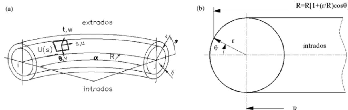
length (s), the mean radius of curvature (R), the thickness (h),the mean section radius of the pipe (r) and the central angle
(a). Fig. 1a shows the essential geometric parameters
defining the two-node finite pipe element. The basic equations governing the behaviour of thin shells were derived by Love [2]. The following assumptions referred to in Refs. [3–5], were considered in the present analysis:
† the radius of curvature is assumed much larger then
the section radius. This means that the ‘pipe bore term’ (RCrcosq) may be approximated toR,Fig. 1b;
† a semi-membrane deformation model is adopted and
neglects the bending stiffness along the longitudinal direction of the toroidal shell, but considers the meridional bending resulting from ovalization;
† the shell is considered thin and inextensible along the
meridional direction in the mechanical case. Typically, the thickness should be less than a tenth of the mean radius of the pipe.
In the mechanical model, having assumed small strains, the complete incremental relation between stress and strain for thermal and mechanical deformation is found to be
3Z3mecC3th (1)
where3mec is the mechanical strain increment and 3ththe thermal strain.
The application of the principle of virtual work gives finally the system of algebraic equations to be solved. The matrix force–displacement equation for this finite pipe element model is
½KfdgZfFngCfFthg (2)
where {d} is a nodal unknown displacement vector, {Fn} is the applied nodal forces and {Fth} is a nodal force vector due to thermal effects. The element stiffness matrix [K] is calculated from the matrix equation:
KZ
ðsZL
sZ0 ðqZ2p
qZ0
½BT½D½Brdsdq (3)
The following expression represents the nodal forces due to the thermal strain
FthZ
ð
V
½BT½Df3gthdV (4)
where dVis the elementary pipe volume, [D] the elasticity matrix and [B] results from the derivative of the shape functions for the pipe element.
Having solved the system of algebraic equations, the displacement field is calculated for all the nodes of the structure. The stress field is then defined for each element in the following form
sZ½Dðf3gmecKf3gthÞCfsg0 (5)
wheres0represents the initial stresses.
The elasticity matrix [D] appears with a simple algebraic definition, where the off-diagonal terms vanish
DZ
Eh
1Kn2 0 0
0 Eh
2ð1CnÞ 0
0 0 Eh
3
12ð1Kn2Þ 2
6 6 6 6 6 6 4
3
7 7 7 7 7 7 5
(6)
where E is the elastic modulus that is a temperature dependent parameter, according to Eurocode3[6],h is the pipe thickness andnis Poisson’s ratio.
3. The displacement field for a new two-node pipe element
The displacements u, v and w are calculated for the shell surface from the structural element. These functions refer to the displacement field on the mean line arc Fig. 1. (a) Geometric parameters for the finite pipe element. (b) The radius of curvature for the curved pipe.
115 116 117 118 119 120 121 122 123 124 125 126 127 128 129 130 131 132 133 134 135 136 137 138 139 140 141 142 143 144 145 146 147 148 149 150 151 152 153 154 155 156 157 158 159 160 161 162 163 164 165 166 167 168
UNCORRECTED PROOF
(U, W and 4). Those parameters are related via simpledifferential equations from beam bending theory, following simple hypotheses considered by Melo and Castro [7,8] and Thomson [5]
4Z
dW
ds (7)
WZK
dU
ds R (8)
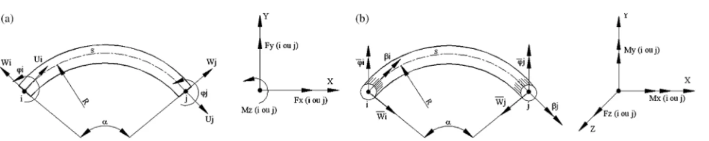
The displacement field is calculated from the mean line of each arc considered like a rigid beam element: U is the tangential displacement, W and W the transverse displacements, b, 4 and 4 are the rotations in each direction represented in Fig. 2a and b, respectively, for in-plane or out-of-plane loading.
When the finite pipe element has in-plane displace-ments, a high-order formulation is used and six par-ameters are necessary to define the displacement field. So, U can be approximated by the following fifth-order polynomial
UðsÞZa0Ca1sCa2s2Ca3s3Ca4s4Ca5s5 (9)
The coefficients in Eq. (9) are determined by imposing boundary conditions according to the curved reference. With those specified conditions, the functions of the generic local displacements for an in-plane element (IN) are given by the following equations:
UðsÞINZðUiNuiCUjNujÞCðWiNwiCWjNwjÞ
Cð4iN4iC4jN4jÞ (10a)
WðsÞINZKRððUiN
0
uiCUjN
0
ujÞCðWiN
0
wiCWjN
0
wjÞ
Cð4iN40iC4jN40jÞÞ (10b)
4ðsÞINZKRððUiN
00
uiCUjN
00
ujÞCðWiN
00
wiCWjN
00
wjÞ
Cð4iN400iC4jN400jÞÞ (10c)
The shape functions are determined as follows:
NuiZcos a 2 C1 Rsin a 2 s
C K10
L3cos
a
2
K 6
RL2sin
a 2 s3 C 15
L4cos a
2
C 8
RL3sin a
2
s4
C K6
L5cos
a
2
K 3
RL4sin
a
2
s5 (11a)
NujZ
10 L3cos
a
2
C 4
RL2sin
a
2
s3
C K15
L4cos a
2
K 7
RL3sin a 2 s4 C 6
L5cos a
2
C 3
RL4sin
a
2
s5 (11b)
NwiZsin a 2 K1 Rcos a 2 s
C K10
L3sin a
2
C 6
RL2cos a 2 s3 C 15
L4sin
a
2
K 8
RL3cos
a
2
s4
C K6
L5sin
a
2
C 3
RL4cos
a
2
s5 (11c)
NwjZ K
10 L3sin
a
2
C 4
RL2cos
a 2 s3 C 15
L4sin
a
2
K 7
RL3cos
a
2
s4
C K6
L5sin
a
2
C 3
RL4cos
a
2
s5 (11d)
N4iZK
1 2Rs
2C 3
2LRs
3K 3
2L2Rs
4C 1
2L3Rs
5 (11e)
UNCORRECTED PROOF
2LR L R 2L R
The displacement field out-of-plane, designated as OUT, in a local reference system, is determined with the following equations:
WðsÞOUTZWiN1K4iN2CWjN3K4jN4 (12a)
4ðsÞOUTZWiN10K4iN20CWjN30K4jN40 (12b)
bðsÞOUTZbiNiCbjNj (12c)
The shape functions used in Eqs. (12a)–(12c) are third-order polynomials (N1, N2, N3, N4) and first-order polynomials (Ni, Nj), respectively.
The surface displacement in the radial direction results from ovalization, in-plane and out-of-plane, from Ref.[5]
and is expressed by the equation:
wðs;qÞZ
X
nR2
ancosnqC
X
nR2
ansinnq
! Ni
C X
nR2
ancosnqC
X
nR2
ansinnq
!
Nj (13)
The meridional displacement due to ovalization is calculated from the following equation:
vðs;qÞZ K
X
nR2
an
n sinnqC X
nR2
an
n cosnq !
Ni
C KX
nR2
an
n sinnqC X
nR2
an
n cosnq !
Nj (14)
Finally, the longitudinal displacement due to warping of the pipe section is defined from the following equation:
uðs;qÞZ
X
nR2
bncosnqC
X
nR2
bnsinnq
! Ni
C X
nR2
bncosnqCX nR2
bnsinnq
!
Nj (15)
The terms an and an are constants to be determined
and included in the Fourier expansions for the ovaliza-tion displacements of in-plane and out-of-plane bending, respectively. The parameters bnandbn are also functions
of developed series resulting from warping displacements in and out-of-plane.
When a tubular system without restraint is subjected to temperature variation, there will be a length increase and the temperature produces dilation along the cross-section of the pipe. The perimeter of the pipe will be variable. Finally, following the proposed formulation, the finite shell element displacement field, resulting from the superposition of
Eqs. (13)–(15), leads to:
uZUðsÞINKrcosq4ðsÞINKrsinq4ðsÞOUTCuðs;qÞCsaDT
(16a)
vZKWðsÞINsinqCWðsÞOUTcosqCrbðsÞOUTCvðs;qÞ
(16b)
wZWðsÞINcosqCWðsÞOUTsinqCwðs;qÞCraDT (16c)
The displacement field of the shell surface in a condensed vector representation is
u v w 8 < : 9 = ; Z u v w 8 < : 9 = ; mec C u v w 8 < : 9 = ; th
Z½N!fdgC
saDT
0
raDT 8 > < > : 9 > = > ; (17)
where a is the thermal expansion coefficient, considered constant in this formulation and DT is the temperature variation.
As referred to previously, the mechanical deformation model considers that the pipe undergoes a semi-membrane strain field. The strain field is given by the following equations also used by Melo and Castro[7,8], Flu¨gge[9]and Kitching[10]
~ 3
mecZ
3ss gsq
cqq 8 < : 9 = ; Z v
vs K
sinq R cosq R 1 r v vq v
vs 0
0 K1
r2 v vq 1 r2 v2 vq2 2 6 6 6 6 6 6 4 3 7 7 7 7 7 7 5 u v w 8 < : 9 = ; (18)
where3ssis the longitudinal membrane strain,gsqis the shear
strain andcqqis the meridional curvature from ovalization.
The dimension of the deformation vector increases one term due to the thermal circumferential deformation by the expression:
3qqZ
1 r wC
vv
vq
Z
raDT
r (19)
The thermal deformation vector is obtained from the following equation: 3ss 3qq th Z aDT
aDT
UNCORRECTED PROOF
Fig. 3. (a) Finite element mesh used in developed program. (b) Displacement nodal results for different temperatures. Deformed shape magnified 30!.
Fig. 4. Expansion of the pipe cross-section using the developed finite pipe element and COSMOS.
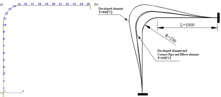
Fig. 5. (a) Geometry of piping system. (b) Mesh used and the thermal and mechanical boundary conditions. 449
450 451 452 453 454 455 456 457 458 459 460 461 462 463 464 465 466 467 468 469 470 471 472 473 474 475 476 477 478 479 480 481 482 483 484 485 486 487 488 489 490 491 492 493 494 495 496 497 498 499 500 501 502 503 504
UNCORRECTED PROOF
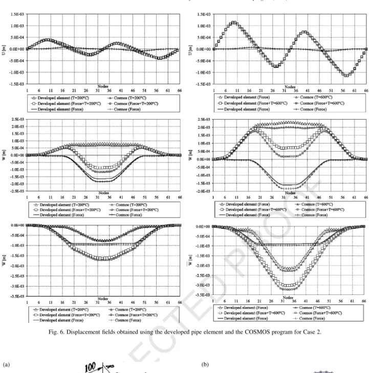
Fig. 6. Displacement fields obtained using the developed pipe element and the COSMOS program for Case 2.Fig. 7. (a) Geometry of piping system. (b) Mesh used and the thermal and mechanical boundary conditions. 563
564 565 566 567 568 569 570 571 572 573 574 575 576 577 578 579 580 581 582 583 584 585 586 587 588 589 590 591 592 593 594 595 596 597 598 599 600 601 602 603 604 605 606 607 608 609 610 611 612 613 614 615 616
UNCORRECTED PROOF
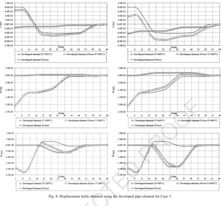
Fig. 8. Displacement fields obtained using the developed pipe element for Case 3.Fig. 9. (a) Geometry of piping system. (b) Mesh used and the thermal and mechanical boundary conditions. 673
674 675 676 677 678 679 680 681 682 683 684 685 686 687 688 689 690 691 692 693 694 695 696 697 698 699 700 701 702 703 704 705 706 707 708 709 710 711 712 713 714 715 716 717 718 719 720 721 722 723 724 725 726 727 728
UNCORRECTED PROOF
4. Case studies4.1. Case 1: a plane geometry piping system subjected to elevated temperatures
A tubular steel piping system has a radius of curvature equal 0.25 m, a mean radius of 0.0135 m and the thickness is 0.001 m,Fig. 3a. The piping system has end restraints and is subjected to different temperatures. The thermal expan-sion coefficienta is constant and equal to 14!10K6
8CK1 ,
nZ0.3 and E is a function of temperature, according to
Eurocode3[6].
The deformed shape obtained is magnified 30! in
Fig. 3b. For a temperature rise of TZ2008C numerical
results have been compared with a commercial code COSMOS using Pipe and Elbow elements as shown in
Fig. 3b.
Fig. 4 represents the transverse displacement obtained
with different temperatures for a section in the tubular
straight pipe for element 5. As can be observed, the pipe cross-section has the mean radius increased with the thermal expansion. The results obtained with the element developed herein are compared with the COSMOS program using a Shell element. This is an advantage with our code; it is possible with the same element to calculate the displace-ment field in the shell surface.
4.2. Case 2: a piping system with spatial geometry subjected to elevated temperatures having two end restraints and a vertical force at the mid-length of the structure
The next case is a structural steel piping system with all elements subjected to uniform temperature (TZ200 or
6008C) and to a vertical force of FZ3000 N, Fig. 5a.
The structure also has end restraints. The system has a mean radius of 0.022 m and a thickness of 0.0025 m. The thermal expansion coefficient is equal to 14!10K68CK1, nZ0.3 and E is a function of temperature, according to
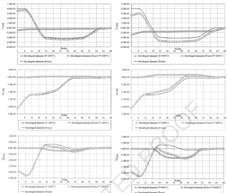
Fig. 10. Displacement fields obtained using the developed pipe element for Case 4. 787
788 789 790 791 792 793 794 795 796 797 798 799 800 801 802 803 804 805 806 807 808 809 810 811 812 813 814 815 816 817 818 819 820 821 822 823 824 825 826 827 828 829 830 831 832 833 834 835 836 837 838 839 840
UNCORRECTED PROOF
Eurocode3 [6]. The finite pipe element mesh uses 65elements as represented in Fig. 5b.
The results are compared with those obtained using the COSMOS programme with Pipe and Elbow elements as shown inFig. 6. We have also compared the influence of the temperature in the structure simultaneously with or without a vertical force.
4.3. Case 3: a piping system with spatial geometry subjected to elevated temperatures having one end restraint
and a vertical force on the other free end
This case is the same as Case 2, but now with the spatial structure subjected to a vertical force,FZ3000 N at one end
and the other end restrained, seeFig. 7a. The structure is subjected to two uniform different temperatures ofTZ200 and 6008C.
The transverse displacement field is influenced by the temperature rise, as shown inFig. 8, having compared these results with those corresponding to the mechanical stand-alone load.
4.4. Case 4: a piping system with spatial geometry subjected to elevated temperatures with upper length zone insulated, having one end restrained and a vertical force on the other free end
The same piping system is now subjected to the same different boundary conditions (vertical force ofFZ3000 N
in free end and the other end restrained, partially subjected to uniform temperature (TZ200 or 6008C) and partially
insulated in the upper length zone AA, seeFig. 9a. The displacement field increases as can be seen in
Fig. 10, compared with the results for Case 3.
5. Conclusions
The results for the structural displacements resulting from elevated temperatures and mechanical actions on
tubular structures have been presented, using a new finite element for linear and elastic formulation. Good agreement between the displacement results obtained with the finite element presented here and corresponding data from other commercial codes was observed. This new two-node finite pipe element presents good agreement in the analysis of thermo-mechanical problems, with all shell membrane capabilities, when compared to other possible finite modelling techniques. It is possible to calculate the displacement field due to elevated temperatures. This finite element is easy to operate, demands small computer capacity and avoids the need to use expensive meshes for the shell surface definition.
References
[1] Fonseca EMM. Finite element analysis of structural piping systems behaviour under high thermal gradients, PhD thesis (in Portuguese), Faculty of Engineering of University of Porto, Porto; 2003. [2] Love AEH. The mathematical theory of elasticity. New York: Dover;
1944.
[3] Madureira L, Melo FQ. A hybrid formulation in the stress analysis of curved pipes. Eng Comput 2000;17(8):970–80.
[4] Fonseca EMM, Melo FJMQ, Oliveira CAM. Determination of flexibility factors on curved pipes with end restraints using a semi-analytic formulation. Int J Press Vessels Piping 2002;79/12:829–40. [5] Thomson G. The influence of end constraints on pipe bends, PhD
Thesis, University of Strathclyde, Scotland, UK; 1980.
[6] CEN ENV 1993-1-2, Eurocode 3: Design of steel structures—Part 1.2: general rules—structural fire design; 1995.
[7] Melo FJMQ, Castro PMST. A reduced integration Mindlin beam element for linear elastic stress analysis of curved pipes under generalized in-plane loading. Comput Struct 1992;43(4):787–94. [8] Melo FJMQ, Castro PMST. The linear elastic stress analysis of curved
pipes under generalized loads using a reduced integration finite ring element. J Strain Anal 1997;32(1):47–59.
[9] Flu¨gge W. Thin elastic shells. Berlin: Springer; 1973.
[10] Kitching R. Smooth and mitred pipe bends. In: Gill SS, editor. The stress analysis of pressure vessels and pressure vessels components. Oxford: Pergamon Press; 1970 [chapter 7].
897 898 899 900 901 902 903 904 905 906 907 908 909 910 911 912 913 914 915 916 917 918 919 920 921 922 923 924 925 926 927 928 929 930 931 932 933 934 935 936 937 938 939 940 941 942 943 944 945 946 947 948 949 950 951 952