Stochastic approach to analyzing the uncertainties and possible changes in the availability of water in the future based on a climate change scenario

(1)

HESSD

12, 3787–3846, 2015

Analyzing the uncertainties and possible changes in

the availability of water

G. G. Oliveira et al.

Title Page

Abstract Introduction

Conclusions References

Tables Figures

◭ ◮

Back Close

Full Screen / Esc

Printer-friendly Version

Interactive Discussion

Discussion

P

a

per

|

Discussion

P

a

per

|

Discussion

P

a

per

|

Discussion

P

a

per

|

Hydrol. Earth Syst. Sci. Discuss., 12, 3787–3846, 2015 www.hydrol-earth-syst-sci-discuss.net/12/3787/2015/ doi:10.5194/hessd-12-3787-2015

This discussion paper is/has been under review for the journal Hydrology and Earth System Sciences (HESS). Please refer to the corresponding final paper in HESS if available.

Stochastic approach to analyzing the

uncertainties and possible changes in the

availability of water in the future based on

a climate change scenario

G. G. Oliveira, O. C. Pedrollo, and N. M. R. Castro

Institute of Hydraulic Research – Federal University of Rio Grande do Sul, Porto Alegre, RS, Brasil

Received: 11 December 2014 – Accepted: 20 March 2015 – Published: 10 April 2015

Correspondence to: G. G. Oliveira (g.g.oliveira10@gmail.com)

(2)

HESSD

12, 3787–3846, 2015

Title Page

Tables Figures

◭ ◮

Back Close

Full Screen / Esc

Discussion

P

a

per

|

Discussion

P

a

per

|

Discussion

P

a

per

|

Discussion

P

a

per

|

Abstract

The objective of this study was to analyze the changes and uncertainties related to water availability in the future (for purposes of this study, it was adopted the period between 2011 and 2040), using a stochastic approach, taking as reference a climate projection from the climate model Eta CPTEC/HadCM3. The study was applied to the

5

Ijuí river basin in the south of Brazil. The set of methods adopted involved, among others, correcting the climatic variables projected for the future, hydrological simulation using Artificial Neural Networks to define a number of monthly flows and stochastic modeling to generate 1000 hydrological series with equal probability of occurrence. A multiplicative type stochastic model was developed in which monthly flow is the result

10

of the product of four components: (i) long term trend component; (ii) cyclic or seasonal component; (iii) time dependency component; (iv) random component. In general the results showed a trend to increased flows. The mean flow for a long period, for in-stance, presented an alteration from 141.6 (1961–1990) to 200.3 m3s−1_{(2011–2040).}

An increment in mean flow and in the monthly SD was also observed between the

15

months of January and October. Between the months of February and June, the per-centage of mean monthly flow increase was more marked, surpassing the 100 % index. Considering the confidence intervals in the flow estimates for the future, it can be con-cluded that there is a tendency to increase the hydrological variability during the period between 2011–2040, which indicates the possibility of occurrence of time series with

20

more marked periods of droughts and floods.

1 Introduction

Discussions concerning variability and climate changes have intensified in the last few decades. Many studies have proved significant alterations in the composition of the atmosphere and, consequently, in the climate-related variables. On this topic the IPCC

25

(3)

estab-HESSD

12, 3787–3846, 2015

Title Page

Tables Figures

◭ ◮

Back Close

Full Screen / Esc

Discussion

P

a

per

|

Discussion

P

a

per

|

Discussion

P

a

per

|

Discussion

P

a

per

|

lished in 1988 by the World Meteorological Organization (WMO) and by the United Nations Environment Program (UNEP) whose objective is to supply scientific informa-tion in order to gain a better understanding of changes in the global climate, so as to evaluate their impact on society and on nature, and propose alternatives for adaptation and mitigation.

5

According to IPCC (2013), it is already clear that the Earth is warming, as proved by the rise in the mean temperatures of the air and the oceans, by the increase in the mean level of the seas and by the acceleration of ice melt in mountain or polar climate regions. Studies developed on a global scale have shown that several natural systems are already under the impact of climate changes.

10

Changes in temperature and precipitation will lead to an increased frequency of ex-treme meteorological events, such as severe floods and droughts, which will inevitably affect the availability of water for human consumption, irrigation, industries and other uses (IPCC, 2013). Some research studies on the sensitivity of agricultural crops to climate changes show that there may be a strong negative effect on crop growth,

in-15

creasing the risk of losses in harvests worldwide (Mearns et al., 1996; Richter and Semenov, 2005; Zhang and Liu, 2005; Rasmussen et al., 2012).

The climate scenario projections are performed using Global Climate Models (GCMs) and Regional Climate Models (RCMs). The resolution of RCMs is between 10 and 50 km, which allow applying them in scenarios of climate changes in medium

20

and small basins. Using these models, together with the GCMs, enables detailing the climate processes at the local level, detecting the variations and specificities of a given region, and thus improving the understanding of impacts in small basins (Marengo et al., 2009, 2012).

The Eta Model was developed at Belgrade University and operationally implemented

25

(4)

HESSD

12, 3787–3846, 2015

Title Page

Tables Figures

◭ ◮

Back Close

Full Screen / Esc

Discussion

P

a

per

|

Discussion

P

a

per

|

Discussion

P

a

per

|

Discussion

P

a

per

|

of Eta Model, Eta CPTEC, was developed independently by the National Institute for Space Research (INPE).

The regional Eta Model was configured over South America and applied to down-scale HadCM3 members of the Perturbed Physics Ensemble (PPE) experiment for the present climate (1961–1990). The dynamic downscaling method was used to generate

5

the climate scenarios (Chou et al., 2012). According to Mujumdar and Kumar (2013), the main advantage of dynamical downscaling over the statistical downscale method is its ability to capture the mesoscale non-linear effects and provide information for many climate variables, while ensuring internal consistency with respect to the physical prin-ciples in meteorology, simulating satisfactorily some regional climatic conditions.

10

The Eta CPTEC Model includes the increase in CO₂concentration levels according to the scenario of emission and daily variation of the state of vegetation during the year. This model reproduces scenario A1B of IPCC SRES, supplied by the global coupled ocean–atmosphere HadCM3, in four members (versions) of disturbance in the global model – (no disturbance – CNTRL; low sensitivity – LOW; medium sensitivity – MID;

15

high sensitivity – HIGH), which represent the uncertainty of boundary conditions, to produce variants of the same model (Chou et al., 2012; Marengo et al., 2012). The regional model was integrated into the horizontal resolution of 40 km, for the period between 1961 and 1990, and the future scenarios were generated in three 30 year periods (from 2011 to 2040, from 2041 to 2070, from 2071 to 2100) (Chou et al., 2012).

20

The study of Marengo et al. (2012) details the scenarios generated for South Amer-ica using the Eta CPTEC/HadCM3 Model. According to this study, the model is con-figured with 38 vertical layers with the top of the model at 25 hPa. The Mellor–Yamada level 2.5 procedure (Mellor and Yamada, 1974) was used for the treatment of tur-bulence. The radiation package was developed by the Geophysical Fluid Dynamics

25

(5)

HESSD

12, 3787–3846, 2015

Title Page

Tables Figures

◭ ◮

Back Close

Full Screen / Esc

Discussion

P

a

per

|

Discussion

P

a

per

|

Discussion

P

a

per

|

Discussion

P

a

per

|

also the NOAH scheme (Ek et al., 2003) to parameterize the land–surface transfer processes (Marengo et al., 2012).

Pesquero (2009), Chou et al. (2012) and Marengo et al. (2012) used Model Eta CPTEC. In the first two studies, the model was used to reproduce the present climate on South America and certify the quality of the model. A smooth tendency was

ob-5

served to underestimate precipitation over the Amazon in the rainy season and the central region of Brazil, in the Brazilian Savanna. In the last study (Marengo et al., 2012), model Eta CPTEC was used to study the climate changes in the Amazon, São Francisco and Paraná river basins between 2011 and 2100.

Currently, in the scientific literature, there are several studies that analyze the effects

10

of climate changes on water availability (examples: Kleinn et al., 2005; Hughes et al., 2011; Gunawardhana and Kazama, 2012). On a continental or global scale, normally, the outputs of the GCMs are used in combination with the empirical macroscale hy-drological models which perform the water balance (for instance, Arnell, 1999, 2004; Nijssen et al., 2001; Milly et al., 2005; Nohara et al., 2006). The studies on water

15

availability in smaller river basins normally use the climate projections for the RCMs, associated with empirical or physically-based hydrological models, in a deterministic approach, offering only a single result in the hydrological sphere for each climate sce-nario. Examples of this are the studies by Middelkoop et al. (2001), Menzel and Bürger (2002) and Kleinn et al. (2005).

20

However, because of the randomness of hydrometeorological processes, the uncer-tainties related to climate modeling and future water availability favor the use of prob-abilistic methods based on stochastic time series, as in the studies by Wilks (1992), Semenov and Barrow (1997) and Booij (2005). The stochastic approach broadens the possibility of analyzing water availability and the climatic uncertainties in the future,

25

(6)

HESSD

12, 3787–3846, 2015

Title Page

Tables Figures

◭ ◮

Back Close

Full Screen / Esc

Discussion

P

a

per

|

Discussion

P

a

per

|

Discussion

P

a

per

|

Discussion

P

a

per

|

However, when generating hundreds or thousands of stochastic climate series, it is necessary to repeat the hydrological simulation often, rendering the modeling pro-cess very onerous from the computational standpoint. Moreover, in this approach the hydrological scenarios produced become even more sensitive to any imprecision in estimating the parameters of the rainfall-flow transformation model.

5

In order to minimize the processing time, this methodology will cover the randomness of the processes and the climate dynamics directly in the flow series, using a stochastic model appropriate for monthly flows. Thus, based on a single climate scenario, a flow series is generated by hydrological deterministic simulation and then the stochastic process is performed.

10

The objective of this study is to analyze the possible scenarios and uncertainties related to water availability in future, using a stochastic approach based on a climatic change scenario originating in the Eta CPTEC/HadCM3 climate model. This study will be applied to the Ijuí river basin, in Rio Grande do Sul (RS), Brazil.

2 Methodology

15

The set of methods adopted in this study comprised the use of observed and simulated hydrometeorological data, to analyze the uncertainties and possible scenarios of water availability in the future, based on a climatic scenario originating in the regional climate model Eta CPTEC/HadCM3.

Simplifying, the methodological procedure covered: (i) spatial interpolation of the

20

meteorological variables; (ii) selection of the climatic scenario and correction of the climate variables; (iii) estimation of the potential evapotranspiration; (iv) hydrological simulation using Artificial Neural Networks (ANNs); (v) stochastic modeling of monthly flows to generate possible hydrological series in the future.

For this study, considering the availability of the climatic data derived from the

re-25

(7)

HESSD

12, 3787–3846, 2015

Title Page

Tables Figures

◭ ◮

Back Close

Full Screen / Esc

Discussion

P

a

per

|

Discussion

P

a

per

|

Discussion

P

a

per

|

Discussion

P

a

per

|

Research – INPE), the years between 1961 and 1990 was considered as a base period and the years between 2011 and 2040 was considered as the “future” period.

2.1 Study Area

This study was applied in the Ijuí River Basin, in the Santo Ângelo stream gauging section, in the northwest of RS, Brazil. The basin area is 5414 km2and it is located

be-5

tween the following geographic coordinates: latitudes 27.98 to 28.74◦_{S and longitudes}

53.21 and 54.28◦_{W (Fig. 1). At this stream gauging station between 1941 and 2005,}

the mean flow (Q) was 138 m3s−1_{, and the dry and high flow periods were the months}

of March (Q=72 m3s−1_{) and October (}_Q

=211 m3s−1_{), respectively.}

The area of the study was chosen because the region depends to a great extent on

10

agricultural activities and may su_ffer serious socioeconomic impacts from the climate changes. According to the State Coordinator of Civil Defense of RS, during the period between 1982 and 2011 there were at least six severe dry periods in the basin region, which caused great losses to the agricultural and cattle activities, mainly those involving soy beans and maize.

15

Considering the daily climate data of the Cruz Alta station, operated by INMET (Na-tional Institute of Meteorology), the winter and spring months (from June to December) are the rainiest. According to Rossato (2011), annual mean precipitation oscillates be-tween 1700 and 1800 mm, bebe-tween 100 and 120 days of rain a year, on average. The annual mean temperature oscillates between 17 and 20◦_{C. The coldest months are} 20

June and July, with a mean of around 14◦_{C, and the warmest months are January and}

February, with a mean of around 24◦_C.

2.2 Data

The following materials were used in this study: (i) daily historical series of precipita-tions provided by the HidroWeb site of the National Water Agency (ANA), during the

25

(8)

cover-HESSD

12, 3787–3846, 2015

Title Page

Tables Figures

◭ ◮

Back Close

Full Screen / Esc

Discussion

P

a

per

|

Discussion

P

a

per

|

Discussion

P

a

per

|

Discussion

P

a

per

|

age of 100 km of the basins boundaries (Fig. 2); (ii) daily historical series of precipitation provided by IPH (Castro et al., 1999), in the years 1989 and 1990, at 22 rain gauging stations (Fig. 2); (iii) daily historical series of precipitation, temperature, wind speed, solar radiation, atmospheric pressure and relative humidity of the air provided through the portal of BDMEP (Bank of Meteorological Data for Teaching and Research) of

IN-5

MET, during the period between 1961 and 1990, at five meteorological stations (Fig. 2); (iv) daily historical series of flows from the Santo Ângelo station, located at coordinates 28.36◦_{S and 54.27}◦_{W, provided through the HidroWeb site, during the period between}

1961 and 1990; (v) daily data simulated by the regional climate model Eta CPTEC, conducted by four members of the global climate model HadCM3, with different levels

10

of sensitivity (CNTRL, LOW, MID and HIGH), during the periods of 1961–1990 (base) and 2011–2040 (“future”). The variables simulated were: precipitation, temperature, wind speed, relative humidity of the air, atmospheric pressure and solar radiation.

2.3 Spatial interpolation

The first stage consisted of the spatial interpolation of the five daily climate variables

15

(temperature, wind speed, relative humidity of the air, atmospheric pressure and solar radiation), and daily precipitation in the periods between 1961–1990 (observed and simulated data) and 2011–2040 (data simulated by the Eta model). The interpolation grid was generated with a spatial resolution of 5 km (Fig. 2), totalizing 264 nodes in the basin area. The interpolation procedure was performed for all data sets: (i) series

20

observed at 104 rain gauging or meteorological stations; (ii) series simulated using model Eta CPTEC/HadCM3 in four scenarios of climate sensitivity (CNTRL, LOW, MID and HIGH).

The use of so many stations in a 100 km radius, to begin the interpolation process consists of a safety margin, since many of these stations present short series, with

25

(9)

HESSD

12, 3787–3846, 2015

Title Page

Tables Figures

◭ ◮

Back Close

Full Screen / Esc

Discussion

P

a

per

|

Discussion

P

a

per

|

Discussion

P

a

per

|

Discussion

P

a

per

|

process. It can be said that for each day, in every node of the interpolation grid, only the closest stations with rainfall data were used, usually within the basin and immediate surroundings.

The interpolation method used was that of the natural neighbor (Sibson, 1981). This interpolation method obtained the best results in the study presented by Silva

5

et al. (2013), with precipitation series similar to those used in the present study, also in the Ijuí River basin. In the study mentioned, the following methods were also tested: closest neighbor, linear triangulation and inverse distance weighting.

The natural neighbor method is based on the concept of area of influence of the sampling points determined by Voronoi polygons. These polygons are obtained from

10

the Delaunay triangulation. For each point on the interpolation grid, the weight of each sampling point is calculated because of the area of influence. The daily value of each variable in the basin was obtained from the mean of the values interpolated in all nodes of the regular grid.

Still at this stage, the daily mean value of the five climate variables and of

precip-15

itation in the Ijuí River basin was calculated, considering the data observed and the data simulated by the ETA model. Finally, the monthly accumulated precipitation for the observed series and for scenarios simulated by the Eta model in the periods of 1961–1990 (base) and 2011–2040 (future) were calculated.

2.4 Selection of climate scenario and correction of climate variables

20

The outputs of climate models should not be used directly to estimate future water availability (Graham, 2000). The climate models may not represent perfectly the current climate due mainly to the influence of the spatial discretization of the models. It is observed (Lenderink et al., 2007) that the outputs may present systematic errors. The correction of climate variables is intended to prevent that the errors intrinsic to the

25

(10)

distur-HESSD

12, 3787–3846, 2015

Title Page

Tables Figures

◭ ◮

Back Close

Full Screen / Esc

Discussion

P

a

per

|

Discussion

P

a

per

|

Discussion

P

a

per

|

Discussion

P

a

per

|

bances (Delta Change Approach) in climate variables is a commonly used strategy to simulate the impacts of climate changes, obtained via global or regional climate mod-els on water resources (Graham, 2004; Lenderink et al., 2007). The technique consists of using only the seasonal change foreseen between the current and future scenario, obtained with the climate model. This change is represented by the difference between

5

the current climatic conditions and those foreseen for the future, both conditions ob-tained by the climate model. The change foreseen is incorporated to the historical series of precipitations and temperature to generate the series in the future. Thus the error associated with climate modeling is eliminated from the current conditions, and becomes limited to the uncertainties associated with the forecast of climate changes

10

for the future. Examples of applying this methodology are the studies by Kaczmarek et al. (1996), Lettenmaier et al. (1999), Graham (2000), Bergström et al. (2001).

However, as mentioned by the authors themselves (Graham, 2000; Bergström et al., 2001), and supported by Lenderink et al. (2007), applying the forecast changes in temperature or in precipitation directly on the series observed implies considerable

15

simplifications which may compromise the analysis of the projections in future. In this approach, for instance, probable changes in the number of rainy days, in dispersion (variance) of rains or in the extreme values of temperature are not considered, since the series itself observed in the past consists of the base of forecasts for the future, and only the seasonal mean variations are taken into account. In this case, there is

20

a risk of considering that the same anomalies recorded in the past will be observed in the future with small changes in the monthly magnitude of climate variables, according to time of the year.

Thus, Lenderink et al. (2007) discuss and analyze how the output of a regional cli-mate model should be corrected to obtain more realistic flows for the current clicli-mate

25

(11)

HESSD

12, 3787–3846, 2015

Title Page

Tables Figures

◭ ◮

Back Close

Full Screen / Esc

Discussion

P

a

per

|

Discussion

P

a

per

|

Discussion

P

a

per

|

Discussion

P

a

per

|

(i) it detects the differences between the current climatic conditions, i.e., between the conditions observed using meteorological stations and the conditions simulated by the regional climate model; (ii) it applies these differences in the series forecast for the future.

Other more sophisticated methods have been tested and compared, with

applica-5

tions at daily or monthly time intervals, as can be seen in Wood et al. (2004), Maurer and Hidalgo (2008), Boé et al. (2007), Piani et al. (2010) and Bárdossy and Pegram (2011). In a recent study, Themeßl et al. (2011) compared a few correction methods and concluded that the Quantile-Based Mapping technique (Panofsky and Brier, 1968) is the most effective one to remove the errors in the precipitation data. This method is

10

applied with small adaptations in the studies listed above. Essentially, the method is based on the differences between the accumulated probability curves (simulated and observed) of daily or monthly precipitations.

In the study by Oliveira et al. (2015a), whose objective was to evaluate the climatic conditions simulated using model Eta CPTEC/HadCM3, emphasizing the study of

wa-15

ter availability in the Ijuí river basin, four methods to correct the climate variables were tested (Delta Change Approach, Direct Approach, Monthly Quantile-Based and Quar-terly Quantile-Based). The control period in which the corrections were applied and the hydrological model calibrated, was defined between 1961 and 1975, and the evaluation period, in which the results of the climate scenarios and water availability were found

20

was 1976 and 1990. For both periods data were available that had been observed at rain gauging stations and meteorological stations and data simulated by the regional climate model Eta CPTEC, conducted by four members of the global climate model HadCM3, with different levels of sensitivity.

The main results obtained in Oliveira et al. (2015a) were: (i) only Eta HIGH did not

25

(12)

er-HESSD

12, 3787–3846, 2015

Title Page

Tables Figures

◭ ◮

Back Close

Full Screen / Esc

Discussion

P

a

per

|

Discussion

P

a

per

|

Discussion

P

a

per

|

Discussion

P

a

per

|

ror 12.6 %) and to the quarterly flow permanence curves (mean error 27.3 %); (iii) with Eta LOW a good adjustment can be seen, both to the low flows (permanence greater than 90 %) and to the high flows (permanence less than 10 %); (iv) the outstanding climate scenario was Eta LOW, applying the Direct Approach correction method, espe-cially as to the curve of permanence of the flows; (v) finally, it was pointed out that in

5

the case of the precipitations and flows the difference between simulated values, based on the Eta model and the values observed was greater than those of evapotranspira-tion, resulting in errors that were sometimes greater than 20 %. One should, therefore, consider that these uncertainties will be reproduced in future scenarios (for the coming decades of the 21st century).

10

Since the present study focuses on a stochastic approach that takes into account the uncertainties associated with the various stages that comprise the modeling of water availability in future, it was necessary to adopt a climate scenario to test the methodol-ogy. Thus, taking into account the results obtained in Oliveira et al. (2015a), the use of the Eta LOW member was defined, applying the Direct Approach correction method.

15

In the Direct Approach method used by Lenderink et al. (2007), the precipitation that is corrected in the future period (2011–2040), in monthk, in year j, is equal to the pre-cipitation simulated during the same period, month and year, multiplied by a correction factor. The correction factor in this method is the ratio between the mean precipitation observed during the base period (1961–1990), in monthk, and the mean precipitation

20

simulated in the same period and month (Eq. 1).

Pcor(fut)_k/j =Psim(fut)_k/j×

h

Pobs(base)_k/Psim(base)_ki (1)

Where: Psim(fut)_k/j is the precipitation simulated during the future period, in month

k and year j;Pobs(base)k is the mean of the precipitation observed during the base period for monthk;Psim(base)k is the mean of precipitation simulated during the base

25

period for monthk.

(13)

HESSD

12, 3787–3846, 2015

Title Page

Tables Figures

◭ ◮

Back Close

Full Screen / Esc

Discussion

P

a

per

|

Discussion

P

a

per

|

Discussion

P

a

per

|

Discussion

P

a

per

|

using Direct Approach, as shown in Eq. (2).

C_Zcor(fut)_{i /k/j} =C_Zsim(fut)_{i /k/j}×

h

C_Zobs(base)_k/C_Zsim(base)_ki (2)

Where:CZcor(fut)i /k/j is the correct value of climate variable z in the future period, in dayi, monthk, and yearj;C_Zsim(f ut)_{i /k/j} is the value simulated of climate variable z during the future period, in dayi, monthk, and yearj;CZobs(base)kis the mean value

5

observed of the climate variablez during the base period for month k;CZsim(base)k is the mean value simulated of the climate variablez during the base period for month

k.

2.5 Estimation of reference evapotranspiration

In the third stage the (daily) reference evapotranspiration was calculated for the

simu-10

lated and corrected climate scenario and for the observed series in the base (1961– 1990) and future (2011–2040) periods. The reference evapotranspiration was calcu-lated using the Penman–Monteith method (Penman, 1948; Monteith, 1965), which has been considered the most reliable method by some authors and was adopted as the standard method by the United National Food and Agriculture Organization (FAO)

15

(Allen et al., 1998). This method is parameterized for an area completely covered with 12 cm high grass, considering the aerodynamic resistance of the surface of 70 s m−1

and albedo of 0.23, in soil without a water deficit.

After calculating the daily evapotranspiration, these values were converted to the monthly time interval, rendering it compatible with the monthly accumulated

precipita-20

tion series for hydrological modeling.

2.6 Hydrological simulation using Artificial Neural Networks (ANNs)

(14)

HESSD

12, 3787–3846, 2015

Title Page

Tables Figures

◭ ◮

Back Close

Full Screen / Esc

Discussion

P

a

per

|

Discussion

P

a

per

|

Discussion

P

a

per

|

Discussion

P

a

per

|

forecasting and classification (Bowden et al., 2005; Jain and Kumar, 2007; Leahy et al., 2008).

The methodology adopted in this study comprised the use of a hydrological model based on ANNs, consisting of transformations of the meteorological and pluviometric variables. The program for the necessary implementation was developed in the

MAT-5

LAB R2010a environment, consisting mainly of a generalized model, constituted by linear transformations of inputs and outputs from a neural network with a hidden layer (Eq. 3).

(y_t−bo)

ao =ANN

₍_x

t−bi) ai

(3)

Where:x_t and y_t are the input and output variables, respectively; ao and bo are the

10

parameters of scale and position of the model outputs; ai and bi are the parameters of scale and position of the model inputs; ANN is the Artificial Neural Network.

The choice of a three-layer architecture was based on the Kolmogorov mapping neu-ral network existence theorem (Hecht-Nielsen, 1987), which stated that any continuous function withninputs can be implemented exactly by a three-layer feedforward neural

15

network with 2n+1 processing elements in the intermediate layer. The ANN is the model core and is represented by Eq. (4):

y=fo

X

h

wofh

X

i

whx+bh

!

+bo

!

+eo (4)

Where:x and y are the matrices with inputs (i) and outputs (o), respectively; wh,bh,

wo andboare the synaptic weight and the tendencies of the hidden layer (h) and the

20

output layer (o), respectively;fh andfo are the activation functions, respectively of the hidden and output layers;eois the expected error at the output layer.

(15)

HESSD

12, 3787–3846, 2015

Title Page

Tables Figures

◭ ◮

Back Close

Full Screen / Esc

Discussion

P

a

per

|

Discussion

P

a

per

|

Discussion

P

a

per

|

Discussion

P

a

per

|

only as a function of the output, and they are represented by Eqs. 5 and 6.

a=f(n)= 1

1+e−n (5)

f′

(n)=a(1−a) (6)

Where:ais the output of the activation function;nis the input value.

The network training was performed through the backpropagation algorithm with

5

crossed validation. This algorithm was proposed by Rumelhart et al. (1986), and con-sists of a method of searching for the synaptic weights to minimize errors, using the so called Delta Rule (Widrow and Hoff, 1960), Eq. (7), which was formulated initially for one-layer neural networks.

W_k₊₁=W_k+(τe_kδ_kP_k) (7)

10

Where:W_k are the current synaptic weights;τis the learning rate;e_k are the errors of outputs from the layers; δk is the derivate of the activation functions; and Pk are the inputs into the layer itself, in iterationk.

In order to apply this method to neural networks with more layers, Eq. (8) is used to estimate the errors in the hidden layers (h), which depend only on the errors and

15

properties of the subsequent layers (s):

eh=

X

(Wsesδs) (8)

Where:e_his the error in the hidden layer;W_sare the synaptic weights in the subsequent layer;esare the errors in the subsequent layer, andδsare the derivates of the activation function in the subsequent layer.

20

(16)

HESSD

12, 3787–3846, 2015

Title Page

Tables Figures

◭ ◮

Back Close

Full Screen / Esc

Discussion

P

a

per

|

Discussion

P

a

per

|

Discussion

P

a

per

|

Discussion

P

a

per

|

in the internal layer was performed using an algorithm that looks at the model perfor-mance after the imposition of small disturbances in the ANN input data.

The initial ANN model was composed of ten input variables, which included precipi-tation and evapotranspiration values at timestand t−1, mean values of precipitation and evapotranspiration in the previous two months, water balance (difference between

5

precipitation and evapotranspiration) and transformed values by applying an exponen-tial decay filter. After the simplification process it was selected a monthly model for the study area, which presents only three input variables, with four neurons in the hidden layer, totalizing 16 synaptic weights. The inputs are: (i) mean water balance at timest

andt−1; (ii) weighted mean of the past values of precipitation by applying an

expo-10

nential decay filter (Hunter, 1986), according to Eq. (9); (iii) weighted mean of the past values of the water balance by applying an exponential decay filter (Eq. 10).

f P_t=(1−α)×f Pt−1+α×Pt. (9)

Where:f P_t and f P_t₋₁ are the values transformed by applying the exponential decay filter to precipitation, at timest and t−1, respectively; Pt is precipitation in time t;α

15

is a coefficient that was calibrated by trials, in order to increase the linear correlation (r) between the filtered variable and the observed flow. In the series used in this study a value equal to 0.52 was obtained for this coe_fficient.

f St=(1−β)×f St−1+β×St. (10)

Where:f S_t and f S_t₋1 are the values transformed by applying the exponential decay

20

filter to the water balance at timest andt−1, respectively;St is the water balance at timet;β is a coe_fficient that was calibrated, similarly to Eq. (9). In the series used in this study, a value equal to 0.41 was obtained for this coefficient.

2.7 Stochastic modeling of monthly flows

According to Salas et al. (1980), if a variable cannot be predicted with certainty, it

25

(17)

HESSD

12, 3787–3846, 2015

Title Page

Tables Figures

◭ ◮

Back Close

Full Screen / Esc

Discussion

P

a

per

|

Discussion

P

a

per

|

Discussion

P

a

per

|

Discussion

P

a

per

|

be defined as stochastic when at least one of the variables involved presents random behavior. According to Salas et al. (1980) the climatic and hydrological variables can be considered random and thus modeled stochastically. In the scientific literature there are numerous references involving the development of stochastic models to generate synthetic climatic and hydrological series (Gabriel and Neumann, 1962; Thomas and

5

Fiering, 1962; Bailey, 1964; Richardson, 1981; Semenov and Barrow, 1997).

In this study a multiplicative type stochastic model was developed to generate monthly flow series. A preliminary analysis of monthly hydrological series was per-formed to examine the stationarity, seasonality and the temporal dependence. Based on this analysis, for this model, it was adopted the assumption that flow may be

esti-10

mated by the result of the product of four components that must be estimated in the following sequence: (i) component of long period tendency (C1), that depends on the position in time, month (m) and year (y); (ii) cyclic or seasonal component (C2), that depends only on the month (m); (iii) time dependence component (C3); (iv) random component (C4). In this model the first three components are modeled

deterministi-15

cally, while the random component (C4), being ruled by probability laws, depends only of the adjustment to any probability distribution function.

The product of the four components (Eq. 11), during all the time intervals of modeling, results in a stochastic sequence of monthly flows (Q_m/y).

Q_m/y=C1_m/y×C2m×C3×C4 (11)

20

In this way, initially, the stochastic modeling process to generate monthly flow series comprised an analysis to look at the stationarity of the observed or simulated series and isolate the tendencies of a long period (C1) This process is necessary to be able to isolate the other components (C2 to C4), both in the base period (1961–1990) and in the future period (2011–2040).

25

(18)

HESSD

12, 3787–3846, 2015

Title Page

Tables Figures

◭ ◮

Back Close

Full Screen / Esc

Discussion

P

a

per

|

Discussion

P

a

per

|

Discussion

P

a

per

|

Discussion

P

a

per

|

months, ranging from 1 to 360). Next, the flow calculated by the linear function (Qtend) is divided by the observed long period mean flow (LPMF), to obtain a correction factor that represents the first component of the model, with a long period tendency (C1), according to Eq. (13). Finally, to obtain a stationary flow (Qst), Eq. (14) was applied, in which the observed flow (Qobs) is divided by component C1.

5

Qtend=0.2459x+98.633 (12)

C1=Qtend

LPMF (13)

Qst=Qobs

C1 (14)

In the series of mean monthly flows simulated during the future period (2011–2040) a linear tendency function was also adjusted, represented by Eq. (15) which calculates

10

flow based only on the time interval (xaxis, in months, ranging from 1 to 360), to remove the tendency found. Then Eqs. 13 and 14 were applied to obtain the stationary series of monthly flows in the future period (2011–2040).

Qtend=0.3105x+143.38 (15)

After defining the long period tendency (C1) for both series (base and future), the other

15

components of the model were estimated based on the stationary series. The cyclic or seasonal component (C2_m) was calculated as the mean of flows in each month (Table 1), in the base (1961–1990) and future periods (2011–2040).

Then the time dependency component was modeled (C3), which represents the in-fluence of the stream values of thepmonths before the flow that occurs in the current

20

(19)

HESSD

12, 3787–3846, 2015

Title Page

Tables Figures

◭ ◮

Back Close

Full Screen / Esc

Discussion

P

a

per

|

Discussion

P

a

per

|

Discussion

P

a

per

|

Discussion

P

a

per

|

In the multiplicative model, component C3 is a non-dimensional factor, with a mean equal to 1 along the hydrological series, obtained by the ratio between observed flow (stationary), in month m, year y, and mean flow in month m (C2_m), as shown by Eq. (16). This equation can only be used when one has observed data. In the case of stochastic modeling, it is assumed that this non-dimensional factor depends only

5

on the value of C3 in the p previous months, thus allowing modeling component C3 at some time interval. The behavior of this component can be modeled by a multiple regression (Eq. 17) or even by a more complex structure, like an ANN with three input variables (Eq. 18).

C3=Qstm/y

C2_m (16)

10

C3_t=f(C3_t₋1, C3t−2, C3t−3) (17)

C3t=RNA(C3t−1, C3t−2, C3t−3) (18)

In this study it was chosen to use a model based on ANNs applying the same algo-rithm detailed in the hydrological modeling stage (Eqs. from 3 to 8), but using as input variables the values of C3 at timest−1,t−2 and t−3, and as expected output the

15

value of C3 at time t. After a few tests and analyses of the results, a neural network was chosen with three neurons in the hidden layer, totalizing 12 synaptic weights.

The random component (C4) is defined as the part that is not explained by the three other deterministic components, i.e., that represents the changes in hydrological be-havior provoked by extreme events that occurred in the month. This part of the monthly

20

flow is represented by the ratio between stationary flow (month, m, year y) and the product of the components C2 (monthm) and C3, as shown by Eq. (19). As in compo-nent C3, the values of C4 tend to a mean value close to 1.

C4= Qestm/y

(20)

HESSD

12, 3787–3846, 2015

Title Page

Tables Figures

◭ ◮

Back Close

Full Screen / Esc

Discussion

P

a

per

|

Discussion

P

a

per

|

Discussion

P

a

per

|

Discussion

P

a

per

|

Next, aiming at the generation of synthetic series, first of all it was checked whether component C4 presented any pattern related to the deterministic portion of the model. Considering the stationary series of the base period (1961–1990), it was found that the value of C4 presented two slightly distinct patterns: (i) when the value of C3 is greater than 1, resulting in flow values higher than the monthly mean in the

determin-5

istic parcel of the model (high flow periods), the tendency of the random component C4 is to present less dispersed values, varying from 0.33 to 2.83, with a slightly lower mean (0.97); (ii) when the value of C3 is lower than 1, resulting in flows lower than the monthly mean in the deterministic portion of the model (low flow periods), the tendency of C4 is to present greater dispersion, varying from 0.21 to 7.24, with a slightly higher

10

mean (1.03).

The most marked oscillations (inflections or impulses) in the monthly hydrogram which depend on the random component C4, occur predominantly in dry periods, when the flow is below the mean observed for the month. This pattern observed in the his-torical series explains the smooth tendency found in the values of this component.

15

Also, considering the stationary series of the future period (2011–2040), when the value of C3 was higher than 1 (high flow periods), the random component C4 presented less dispersed values, ranging from 0.24 to 2.46, with a slightly lower mean (0.99). On the other hand, when the value of C3 was less than 1 (dry periods), component C4 oscillated between 0.13 and 4.98, with a mean of 1.06.

20

Once the probability curves observed in both periods (base and future) had been observed, a few statistical distributions were adjusted (Gamma, Log-Normal, Weibull, among others) to the values of the random component C4. After the Kolmogorov– Smirnov adherence test was performed, it was found that the Gamma probabilities distribution with three parameters presented the best adjustment to the component

25

modeled. The Gamma distribution with three parameters (ϑ,η,β) is represented by the function given by Eq. (20).

f_X(x)=ζ

η−1_e−ζ

ϑΓ(η) , comζ=

x−β

(21)

HESSD

12, 3787–3846, 2015

Title Page

Tables Figures

◭ ◮

Back Close

Full Screen / Esc

Discussion

P

a

per

|

Discussion

P

a

per

|

Discussion

P

a

per

|

Discussion

P

a

per

|

Where:ϑis a parameter of scale, with the dimensionx;βis is a parameter of position, whereβ < x <∞, representing the smallest value ofx;ηis a shape parameter;Γ(η) is the Gamma function, normally solved by numerical integration.

After the adjustment of the four components, the stochastic series for both periods were generated, referenced to the parameters calculated based on the two monthly

5

flow series (observed between 1961 and 1990, and simulated between 2011 and 2040). One thousand series with an equal probability of occurrence were generated for each period.

The stochastic modeling process was evaluated comparing the series generated and the series simulated in the future period, from the following aspects: (i) mean monthly

10

flows; (ii) long period mean flow and volume discharged; (iii) SD of monthly flows; (iv) permanence curves.

The changes and uncertainties in water behavior were evaluated by comparing the stochastic series generated for the future period (2011–2040) and the series generated for the base period (1961–1990), considering central values and limits of confidence,

15

looking at the following aspects: (i) mean monthly flows; (ii) SD of monthly flows; (iii) long period mean flow and volume discharged; (iv) permanence curves.

3 Results and discussions

This item will present the results and the discussions held concerning the analysis of stochastic modeling of monthly flows and the changes and uncertainties in water

20

availability in the future period, between 2011 and 2040.

3.1 Analysis of stochastic modeling of monthly flows

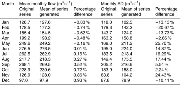
The stochastic series generated preserved several characteristics of the original se-ries, simulated for the period between 2011 and 2040. Considering the mean of the 1000 series generated for the future period, the long period mean flow (LPMF) was

(22)

HESSD

12, 3787–3846, 2015

Title Page

Tables Figures

◭ ◮

Back Close

Full Screen / Esc

Discussion

P

a

per

|

Discussion

P

a

per

|

Discussion

P

a

per

|

Discussion

P

a

per

|

200.3 m3s−1_{, only 1.1 m}3_s−1 _{(0.5 %) more than the simulated LPMF (original series).}

This result was also reflected in the accumulated curve of volume discharged (Fig. 3), where the mean di_fference between the simulated curve (original series) and the cen-tral tendency of the 1000 curves generated (stochastic series) was only 4.8 %. Further-more it can be seen that the smooth tendency of a long period was also preserved, and

5

the values grew more markedly in the final half of the period.

Another characteristic maintained from the original series was the mean monthly flow. Considering the mean of the 1000 series generated for the period between 2011 and 2040 the mean absolute di_fference was only 0.52 % (Table 2). The greatest ab-solute difference between mean flows occurred in October, with an overestimation of

10

1.65 m3s−1_.

Table 2 also shows that the monthly SD was reasonably preserved, with a mean percentage absolute difference of 13.9 % between the original series and the central tendency of the 1000 series generated. The smallest difference was found in the month of October, of only 4.12 m3s−1 _{(2.2 %). The greatest di}

fference as to the monthly SD

15

was found in the month of May (43.2 m3s−1_{), equivalent to 25.7 %.}

Figure 4 illustrates the permanence curves of the mean monthly flow in the future period (2011–2040), in which the similarity between the original series and the central tendency observed in the stochastic series generated becomes clear. The greatest differences were observed in the extremely high flows, with a permanence of less than

20

2 %. In the rest of the permanence intervals the original curve was always located at the 90 % confidence interval defined by the red lines on the graph.

3.2 Analysis of changes and uncertainties in water availability

The first aspect analyzed as to changes and uncertainties regarding water availability in the future refers to the long period mean flow (LPMF) and to the volume discharged

25

(23)

HESSD

12, 3787–3846, 2015

Title Page

Tables Figures

◭ ◮

Back Close

Full Screen / Esc

Discussion

P

a

per

|

Discussion

P

a

per

|

Discussion

P

a

per

|

Discussion

P

a

per

|

in the period, with a significance level of 0.1, was between 123.7 and 162.3 m3s−1

(range 38.6 m3s−1_{). On the other hand, in the future period (2011–2040), the projected}

LPMF was 200.3 m3s−1_{, considering the mean value found in the series. This value}

represents a mean increase of 41.4 % in the LPMF. The confidence interval of LPMF in the future, considering the same level of significance, will be between 165.1 and

5

233.6 m3s−1_{. Thus, the range of the interval will increase from 38.6 to 68.6 m}3_s−1_.

The change of LPMF according to the projection for the future is also reflected by the mean of the total volume discharged over a 30 year period. Between the years of 1961 and 1990 the mean of the total volume discharged was 132 566 Hm3. On the other hand, in the future period (2011–2040) the same volume was surpassed on average in

10

22 years and 10 months. The mean total volume discharged between 2011 and 2040 was 185 869 Hm3(Fig. 5).

Considering the stochastic series in the future period, at a 0.1 level of significance, the total volume discharged at the end of 30 years is at the interval between 154 014 Hm3and 218 002 Hm3. This interval is broader and presents values much superior to

15

those observed in the base period, whose total volume varied between 115 462 Hm3 and 151 454 Hm3for the same limit of confidence (Fig. 5).

The second aspect analyzed refers to mean monthly flows. Fig. 6 presents the mean and the 90 % confidence interval for the mean monthly flows, considering the 1000 stochastic series generated during the base and future periods.

20

The mean monthly flow will increase between the months of January and October, during the period between 2011 and 2040, compared to the base period (1961–1990), with percentages that vary from 14.7 (August) to 118.2 % (March). Besides the month of March, at least four other months will present a significant increase of mean flow: (i) February (113.3 %); (ii) May (110 %); (iii) April (100.7 %); (iv) June (74.1 %).

Consid-25

(24)

HESSD

12, 3787–3846, 2015

Title Page

Tables Figures

◭ ◮

Back Close

Full Screen / Esc

Discussion

P

a

per

|

Discussion

P

a

per

|

Discussion

P

a

per

|

Discussion

P

a

per

|

percentages of 24.3 and 21 %, respectively, will only occur in the months of November and December.

Considering a statistical analysis of the 1000 stochastic series generated for the two periods analyzed (base and future), at a 0.1 level of significance the confidence interval can be estimated which comprises the mean flow of each month (Fig. 6). The greater

5

the range of this interval, the greater also the uncertainty related to the mean monthly flow.

The range of the 90 % confidence interval for the mean monthly flows will only be reduced in the months of November and December, thus following the tendency ob-served in the mean monthly values. In November, for instance, the mean flow in the

10

base period, considering the series generated, was between 134.2 and 209.7 m3s−1

(range of 75.5 m3s−1_{). On the other hand, in the future period, the mean flow of the}

month of November is placed in the interval between 97.2 and 160.7 m3s−1_{(range of}

63.6 m3s−1_{), a reduction of 11.9 m}3_s−1_{in the interval (15.8 %). In December, the range}

of the 90 % confidence interval for mean flow was reduced by 13.5 %, considering the

15

two periods.

In all other months, the range of the confidence interval increased in the future, par-ticularly between the months of February and June, with a greater percentage than 100 %, indicating greater variability between the stochastic series generated and, con-sequently, greater uncertainties in estimating mean flow. The month of May presented

20

the greatest change in this sense. The mean flow during the base period, considering a 90 % confidence interval was between 95.3 and 144.9 m3s−1 _{(range of 49.6 m}3_s−1_).

On the other hand, in the future period, the mean flow in May is inserted into the in-terval between 187.4 and 314 m3s−1_{(range of 126.6 m}3_s−1_{), a 76.9 m}3_s−1_{increase in}

the interval (+155 %).

25

(25)

HESSD

12, 3787–3846, 2015

Title Page

Tables Figures

◭ ◮

Back Close

Full Screen / Esc

Discussion

P

a

per

|

Discussion

P

a

per

|

Discussion

P

a

per

|

Discussion

P

a

per

|

the interval found in the base period is smaller than the lower limit of the interval found in the future.

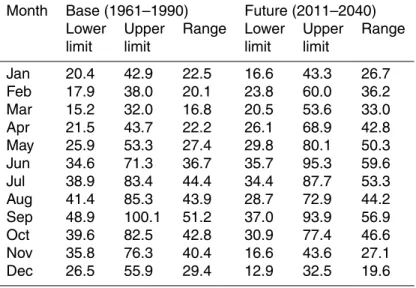
The third aspect analyzed in the hydrological comparison between the base (1961– 1990) and future period (2011–2040) was the SD of mean monthly flows (Table 3). As in the case of the average of the flows in each month, considering the central tendency

5

of the 1000 series generated in the two periods, the SD should increase between the months of January and October, indicating a significant increase in the dispersion of flow values in these months.

The period of the year between the months of February and July is that one where the greatest change occurs in the dispersion of the flow values. In May, for instance, the SD

10

is changed from 82.9 (1961–1990) to 211.2 m3s−1_{(2011–2040), which is a 154.8 %}

in-crease for the future (Table 3). On the other hand, the month of November presents a smooth tendency to reduction in the flows with a 121 reduction to 104.2 m3s−1

(₋13.9 %).

When dividing the monthly SD by the mean monthly flow, the coefficients of

vari-15

ation (CV) were obtained for both series, for each month. It can be seen that during the base period (1961–1990), the CV oscillated between 0.698 (February) and 0.716 (November), while in the future period (2011–2040), the same index varied between 0.801 (April) and 0.848 (May). These results indicate a real increase of the monthly variability of flows, with greater fluctuations of monthly flows in the future.

20

Another aspect analyzed as to changes in hydrological behavior in the future refers to permanence curves of mean monthly flows. Figures 7 and 8 respectively illustrate the mean value and confidence interval of 90 % for the permanence curves of monthly flow, considering the 1000 stochastic series generated in the base (1961–1990) and future periods (2011–2040).

25

(26)

HESSD

12, 3787–3846, 2015

Title Page

Tables Figures

◭ ◮

Back Close

Full Screen / Esc

Discussion

P

a

per

|

Discussion

P

a

per

|

Discussion

P

a

per

|

Discussion

P

a

per

|

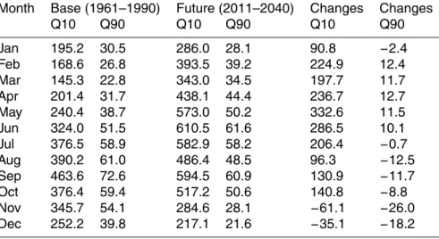
to estimate the maximum possible flow to be regularized. Flow rates with probability of exceedance equal to or less than 10 % (Q10, Q5) are used in studies related to extreme flood events.

The flow will be reduced in the future period only at permanence intervals greater than 91 %, i.e., in the portion of lower flows which characterize dry periods. For flows

5

with a permanence equal to or less than Q90 (intermediate and high flow), the tendency is toward increase in the flow values (Fig. 7). As to the range of the 90 % confidence interval for the permanence curve of monthly flows (Fig. 8), the tendency is to increase in the future period, even the lower flows portion. This result illustrates an increase in the uncertainties associated with the estimate of the permanence curve in the future.

10

On average, considering all the series generated during the base (1961–1990) and future periods (2011–2040), flow with a probability of exceedance equal to or less than 99 % of the months (Q99) was 17.8 and 15 m3s−1_{, respectively. This indicates a mean}

reduction of 15.8 % in Q99 for the future period. Considering a statistical analysis of the stochastic series, at a 0.1 level of significance, we can say that Q99, during the period

15

between 1961 and 1990, is located at the interval between 13.7 and 22.3 m3s−1_{, with}

a range of 8.6 m3s−1

. On the other hand in the future period (2011–2040) this interval changes to values between 10.4 and 20.4 m3s−1_{, with a range of 9.9 m}3_s−1_.

On average, considering all the series generated during the base (1961–1990) and future periods (2011–2040), flow with a probability of exceedance equal to or less than

20

95 % of the months (Q95) was 30 and 28.5 m3s−1_{, respectively. This indicates a mean}

reduction of 1.5 m3s−1₍

−5.1 %) in Q95 for the future period. This percentage is lower than that observed in Q99, illustrating the tendency to inversion in the permanence curves for larger flows. As for the confidence interval of 90 % of Q95, during the pe-riod between 1961 and 1990, the range was 10.4 m3s−1_{, with flows between 25 and} 25

35.4 m3s−1_{. On the other hand in the future period (2011–2040) this interval lies}

be-tween 22.4 and 35.8 m3s−1_{, with a range of 13.4 m}3_s−1_.

(27)

HESSD

12, 3787–3846, 2015

Title Page

Tables Figures

◭ ◮

Back Close

Full Screen / Esc

Discussion

P

a

per

|

Discussion

P

a

per

|

Discussion

P

a

per

|

Discussion

P

a

per

|

shows a mean increase of 0.9 m3s−1 _{(2.2 %) in Q90 for the future period. As to the}

confidence interval of 90 % of Q90 in the period between 1961 and 1990, the range was 12.4 m3s−1_{, with flows between 33.8 and 46.2 m}3_s−1_{. On the other hand in the}

future period (2011–2040) this interval is between 32.4 and 50.8 m3s−1_{, with a range}

of 18.4 m3s−1_. 5

In the base period (1961–1990), on average, the flow with a probability of ex-ceedance equal to or less than 50 % of the months (Q50) was 108.2 m3s−1_{. At a 0.1}

significance level, it can be said that Q50 in this period is inserted into the interval between 94.6 and 122.9 m3s−1_{, with a range of 28.2 m}3_s−1_{. On the other hand in the}

future period, on average, the Q50 was much higher, with a values of 145.1 m3s−1_, 10

indicating a mean increase of 34.2 % for the future. As to the confidence interval, it can be said that the Q50, between 2011 and 2040, will be between 115.8 and 178.1 m3s−1

(range of 62.3 m3s−1_{). Thus, the di}

fferences between the confidence intervals of Q50 in the two periods indicate a significant increase in the uncertainties associated with the permanence of flows in future. These results also illustrate a tendency to an increase

15

in the differences between the flows of the base period and the future period inversely proportional to permanence.

In the portion of flows with permanence between 5 (Q5) and 30 % (Q30), the confi-dence intervals (0.1 significance) of the two periods do not overlap, i.e., the upper limit of the interval during the base period is smaller than the lower limit of the interval in

20

a future period. In the other portions of flows, even if significant differences have been found between the confidence intervals estimated in the base and future periods, they present an overlapping area.

Finally, the changes in the permanence curves of the mean monthly flows in the future, individually, for each month were analyzed. Comparing the permanence curves

25

in the two periods – base (1961–1990) and future (2011–2040) – it can be seen that the smallest changes observed occurred between August and January. In December the absolute mean difference between the permanence curves was 26.1 m3s−1_{, and}