Level 0 to 1 processing of the imaging Fourier transform spectrometer GLORIA: generation of radiometrically and spectrally calibrated spectra

(1)

AMTD

7, 2827–2878, 2014

Level 0 to 1 processing of

GLORIA

A. Kleinert et al.

Title Page

Abstract Introduction

Conclusions References

Tables Figures

◭ ◮

Back Close

Full Screen / Esc

Printer-friendly Version Interactive Discussion

Discussion

P

a

per

|

D

iscussion

P

a

per

|

Discussion

P

a

per

|

Discuss

ion

P

a

per

|

Atmos. Meas. Tech. Discuss., 7, 2827–2878, 2014 www.atmos-meas-tech-discuss.net/7/2827/2014/ doi:10.5194/amtd-7-2827-2014

Atmospheric Measurement

Techniques

Open Access

Discussions

This discussion paper is/has been under review for the journal Atmospheric Measurement Techniques (AMT). Please refer to the corresponding final paper in AMT if available.

Level 0 to 1 processing of the imaging

Fourier transform spectrometer GLORIA:

generation of radiometrically and

spectrally calibrated spectra

A. Kleinert1, F. Friedl-Vallon1, T. Guggenmoser2, M. Höpfner1, T. Neubert3, R. Ribalda3,*, M. K. Sha1, J. Ungermann2, J. Blank2,**, A. Ebersoldt4, E. Kretschmer1, T. Latzko1, H. Oelhaf1, F. Olschewski5, and P. Preusse2

1

Institut für Meteorologie und Klimaforschung, Karlsruher Institut für Technologie, Karlsruhe, Germany

2

Institut für Energie und Klimaforschung – Stratosphäre, Forschungszentrum Jülich, Jülich, Germany

3

Zentralinstitut für Engineering, Elektronik und Analytik-Systeme der Elektronik (ZEA-2), Forschungszentrum Jülich, Jülich, Germany

4

Institut für Prozessdatenverarbeitung und Elektronik, Karlsruher Institut für Technologie, Karlsruhe, Germany

5

Fachbereich C – Atmosphärenphysik, Bergische Universität Wuppertal, Wuppertal, Germany

*

(2)

AMTD

7, 2827–2878, 2014

GLORIA

A. Kleinert et al.

Title Page

Tables Figures

◭ ◮

Back Close

Full Screen / Esc

Discussion

P

a

per

|

D

iscussion

P

a

per

|

Discussion

P

a

per

|

Discuss

ion

P

a

per

|

**

now at: Google Inc., Dublin, Ireland

Received: 24 February 2014 – Accepted: 17 March 2014 – Published: 25 March 2014

Correspondence to: A. Kleinert (anne.kleinert@kit.edu)

(3)

AMTD

7, 2827–2878, 2014

GLORIA

A. Kleinert et al.

Title Page

Tables Figures

◭ ◮

Back Close

Full Screen / Esc

Discussion

P

a

per

|

D

iscussion

P

a

per

|

Discussion

P

a

per

|

Discuss

ion

P

a

per

|

Abstract

The Gimballed Limb Observer for Radiance Imaging of the Atmosphere (GLORIA) is an imaging Fourier transform spectrometer that is capable of operating on various high altitude research aircraft. It measures the atmospheric emission in the thermal infrared spectral region in limb and nadir geometry. GLORIA consists of a classical Michelson

5

interferometer combined with an infrared camera. The infrared detector has a usable range of 128_×128 pixels, measuring up to 16 384 interferograms simultaneously.

Imaging Fourier transform spectrometers impose a number of challenges with re-spect to instrument calibration and algorithm development. The innovative optical setup with extremely high optical throughput requires the development of new methods and

10

algorithms for spectral and radiometric calibration. Due to the vast amount of data there is a high demand for scientifically intelligent optimisation of the data processing.

This paper outlines the characterisation and processing steps required for the gen-eration of radiometrically and spectrally calibrated spectra. Methods for performance optimisation of the processing algorithm are presented. The performance of the data

15

processing and the quality of the calibrated spectra are demonstrated for measure-ments collected during the first deploymeasure-ments of GLORIA on aircraft.

1 Introduction

The upper troposphere/lower stratosphere (UTLS) is a region of particular importance for radiative forcing. Especially uncertainties of exchange processes between the

trop-20

ical upper troposphere and the lowermost stratosphere are a major error source in the Earth radiation budget (Riese et al., 2012). In a more general sense, transport pathways of air between diﬀerent compartments of the atmosphere aﬀecting dynamics and chemistry in a changing climate need to be studied more thoroughly. In order to fully understand these processes, measurements are required which provide both high

25

(4)

AMTD

7, 2827–2878, 2014

GLORIA

A. Kleinert et al.

Title Page

Tables Figures

◭ ◮

Back Close

Full Screen / Esc

Discussion

P

a

per

|

D

iscussion

P

a

per

|

Discussion

P

a

per

|

Discuss

ion

P

a

per

|

The Gimballed Limb Observer for Radiance Imaging of the Atmosphere (GLORIA) is an airborne imaging Fourier Transform Spectrometer (FTS) representing the first reali-sation of the infrared-emission limb-imaging technique (Riese et al., 2005; Friedl-Vallon et al., 2006). It is designed to measure two- and three-dimensional trace gas distribu-tions in the UTLS region with high spatial resolution (Friedl-Vallon et al., 2014). For this

5

purpose GLORIA combines a classical Michelson interferometer with a detector array providing a good spatial coverage and resolution together with a good spectral resolu-tion and a suﬃcient signal-to-noise ratio. It is deployed in the belly pod of the German research aircraft HALO as well as on board the Russian high altitude research plane M55 Geophysica.

10

The transition from a single detector FTS to a 2-D imaging FTS requires new meth-ods in data evaluation and exploitation. The optical throughput of such a system is much higher than the throughput of a conventional FTS, allowing larger spatial cover-age and higher sensitivity with a smaller instrument. As a challenge, such an instrument setup leads to diﬀerent spectrometric properties for each pixel. In particular, the

spec-15

tral axis is diﬀerent for each pixel and new methods for an accurate spectral calibration are required in order to allow for a coherent scientific interpretation of diﬀerent pixels.

In principle, each detector element together with the interferometer is an independent spectrometer. Properties like sensitivity, linearity, and spectral cut-oﬀof these several thousand independent spectrometers may vary randomly from pixel to pixel and/or

20

systematically over the detector array. These properties have to be characterised and considered during calibration. Furthermore, an imaging FTS delivers much more data than a conventional spectrometer. This requires intelligent and eﬃcient strategies for data processing.

This paper describes the level 0 and level 1 processing for GLORIA. Level 0

process-25

(5)

AMTD

7, 2827–2878, 2014

GLORIA

A. Kleinert et al.

Title Page

Tables Figures

◭ ◮

Back Close

Full Screen / Esc

Discussion

P

a

per

|

D

iscussion

P

a

per

|

Discussion

P

a

per

|

Discuss

ion

P

a

per

|

described in detail in Sect. 5. Section 6 deals with the performance optimisation of the processor. The characterisation and processing results for scientific flights performed in 2012 are finally presented in Sect. 7.

2 GLORIA instrument and data acquisition

The GLORIA spectrometer is a cooled imaging FTS with a large cryogenic HgCdTe

5

detector array for the detection of infrared radiation in the spectral range of 780 to 1400 cm−1_{. The spectrometer is mounted in a gimballed frame that allows limited agility} in azimuthal, elevational and image rotation direction. The instrument is designed to measure in limb or nadir viewing geometry. In addition, the centre of the FOV can be directed to an elevation of about +10◦ _{for the so-called deep space view and into}

10

two large area blackbodies for radiometric calibration. A detailed description of the instrument is given by Friedl-Vallon et al. (2014).

The heart of the FTS is a classical Michelson interferometer with a maximum optical path diﬀerence (MOPD) of_±9 cm. The interferogram length can be chosen freely within this range. Two principal measurement modes have been used for limb measurements:

15

– Thechemistry modewith focus on the atmospheric composition has an MOPD of

±8 cm and a spectral sampling of 0.0625 cm−1.

– Thedynamics mode with focus on small-scale dynamics of the atmosphere has

an MOPD of_±0.8 cm and a spectral sampling of 0.625 cm−1. The shorter interfer-ograms in the dynamics mode enable a higher horizontal sampling.

20

The optical interferometer velocity is set to 1.27 cm s−1, leading to an interferogram acquisition time of about 12 s in chemistry mode and 1.2 s in dynamics mode, plus a turnaround time of 0.8 s in both modes.

The infrared detector is an HgCdTe large focal plane array (LFPA) consisting of 256_×256 pixels with a pitch of 40 µm and a stare-while-scan readout. Eight channels

(6)

AMTD

7, 2827–2878, 2014

GLORIA

A. Kleinert et al.

Title Page

Tables Figures

◭ ◮

Back Close

Full Screen / Esc

Discussion

P

a

per

|

D

iscussion

P

a

per

|

Discussion

P

a

per

|

Discuss

ion

P

a

per

|

of 14 bit ADCs, synchronously clocked with 10 MHz on a separate frontend electronics, perform the digitalisation of the LFPA output.

For the GLORIA measurements, only a subset of the array is actually used. The optics is designed to cover a square of 128_×128 pixels, but the typical flight configu-ration in the current setup uses only 48 pixels horizontally and 128 pixels vertically for

5

an optimised interferogram sampling frequency. With this configuration, the sampling frequency or frame rate is 6281 Hz resulting in a detector raw data rate of 73.6 MiB s−1 by using a 16-bit-wide-integer value representation.

Each frame is marked with a unique time stamp by the interferometer electronics, and all frames of an interferogram are gathered into so-called data cuboids. The cuboids

10

are transferred to the central computer where they are written onto a high speed RAID-system (Neubert et al., 2014).

The optical path diﬀerence of the interferometer is measured with a laser reference system. A diode laser signal with a wavelength of about 646 nm is coupled into the interferometer, and the rising zero crossings of the laser interferogram are detected

15

and marked with a time stamp. These time stamps are stored as laser data files. The time stamps for both the infrared and the laser signal are generated by a 80 MHz clock within the interferometer electronics. They are given in integer time ticks with one tick corresponding to 12.5 ns.

Each measurement consists of one cuboid containing the infrared signal sampled

20

(7)

AMTD

7, 2827–2878, 2014

GLORIA

A. Kleinert et al.

Title Page

Tables Figures

◭ ◮

Back Close

Full Screen / Esc

Discussion

P

a

per

|

D

iscussion

P

a

per

|

Discussion

P

a

per

|

Discuss

ion

P

a

per

|

3 Radiometric calibration

3.1 Calibration approach

The radiometric calibration assigns absolute radiance units to the arbitrary intensity units of the measured spectra and the instrument self-emission contributing to the measured spectra is determined and subtracted from the signal. For a sound trace gas

5

retrieval, the goal requirement for the radiometric gain accuracy is 1 % with a threshold of 2 % (Friedl-Vallon et al., 2014).

The standard approach for radiometric calibration is to look at two blackbodies with diﬀerent temperatures. Assuming a linear system, gain g and oﬀsetocan be derived from these two measurements (see, e.g., Revercomb et al., 1988):

10

g=Sh−Sc Bh−Bc

(1)

o=Sc

g −Bc (2)

Sh and Sc are the measured spectra of the hot and cold blackbody, respectively, and BhandBcare the corresponding radiance spectra which are calculated from the

black-15

body temperatures following Planck’s law. The calibrated spectrumL_atmis then calcu-lated from the measured spectrumSatmusing

Latm= Satm

g −o (3)

The two-point calibration approach is only valid if the detected signal is linear with

20

(8)

AMTD

7, 2827–2878, 2014

GLORIA

A. Kleinert et al.

Title Page

Tables Figures

◭ ◮

Back Close

Full Screen / Esc

Discussion

P

a

per

|

D

iscussion

P

a

per

|

Discussion

P

a

per

|

Discuss

ion

P

a

per

|

For the radiometric calibration of the data measured by GLORIA, two large-area blackbody radiation sources (126 mm_×126 mm) are flown on the aircraft. The black-bodies are mounted outside of the spectrometer placing all optical elements including the spectrometer entrance window within the light path during the calibration measure-ments. The blackbodies are temperature stabilised using thermo-electric coolers which

5

allow likewise heating and cooling. Basic requirements are an emissivity of larger than 0.997 and a temperature homogeneity and knowledge of better than 0.1 K in order to achieve the radiometric accuracy goal for the calibrated spectra. Details of the black-body design are given by Olschewski et al. (2013).

The blackbody measurements are complemented by so-called deep space

measure-10

ments, where the instrument is looking upwards into space with an elevation angle of

+₁₀◦_{. Deep space is a commonly used cold calibration source for satellite} measure-ments, because it directly gives the instrument self-emission. This is not entirely true for airborne measurements because of residual emission from trace gases above flight al-titude. These residual atmospheric signatures have to be removed from the measured

15

deep space signal in order to get the instrument self-emission. A method for the re-moval of atmospheric lines from deep space measurements is presented in Sect. 3.3. So in fact three calibration points are available for GLORIA measurements.

A typical calibration sequence in flight consists of 20 hot and 20 cold blackbody measurements, followed by 10 deep space measurements. Blackbody measurements

20

are performed with the dynamics mode spectral resolution, deep space measurements with the chemistry mode spectral resolution. For an optimised signal-to-noise ratio, the detector integration time is adjusted to the intensity of the source, i.e. the integration time for blackbody measurements is shorter than the integration time for atmospheric and scene measurements.

25

(9)

AMTD

7, 2827–2878, 2014

GLORIA

A. Kleinert et al.

Title Page

Tables Figures

◭ ◮

Back Close

Full Screen / Esc

Discussion

P

a

per

|

D

iscussion

P

a

per

|

Discussion

P

a

per

|

Discuss

ion

P

a

per

|

calibration sequence, about 10 to 15 % of the available measurement time is currently used for calibration.

In principle, only two of the three calibration sources are needed to calculate gain and oﬀset. The combination of any two of the three sources should give the same results. In reality, diﬀerences can be found due to

5

1. a non-perfect non-linearity correction

2. errors in the temperature and emissivity of the blackbodies

3. a non-perfect removal of atmospheric contributions to the deep space measure-ments

4. measurement noise.

10

During the flights performed so far, the ambient temperature in the belly pod of the aircraft was typically 245 to 260 K and thus considerably above the outside air tempera-ture, limiting the cooling of the cold blackbody. This led to a relatively small temperature difference of typically only 15 to 25 K instead of the target value of 40 K. The small tem-perature difference and thus the small difference in the measured blackbody spectra

15

(Sh−Sc) makes the blackbody-blackbody calibration very susceptible to measurement

noise, and the extrapolation to zero input, which is needed to determine the instrument oﬀset, is critical. Therefore the current baseline is to use primarily the cold blackbody and the deep space measurements for calibration. The additional data of the hot black-body can be used to check the data for consistency and to enhance the data quality

20

(10)

AMTD

7, 2827–2878, 2014

GLORIA

A. Kleinert et al.

Title Page

Tables Figures

◭ ◮

Back Close

Full Screen / Esc

Discussion

P

a

per

|

D

iscussion

P

a

per

|

Discussion

P

a

per

|

Discuss

ion

P

a

per

|

Using a blackbody-deep space calibration, Eqs. (1) and (2) are simplified to

g=Sbb−Sds Bbb

(4)

o=Sds

g (5)

where bb and ds denote the (cold) blackbody and deep space measurements,

respec-5

tively.

3.2 Non-linearity correction

The detector system exhibits a certain non-linearity, i.e. the output signal is not directly proportional to the input signal. It is assumed that the photovoltaic detector itself is basically linear, and the non-linearity mainly stems from the readout electronics. The

10

non-linearity is characterised by varying the integration time and therewith the num-ber of recorded electrons while looking at a constant radiation source (Hilnum-bert, 2004; P. Giaccari, personal communication, 2010). The recorded DC values are mapped on a virtual detector system, which is linear, i.e. the output signal is directly proportional to the integration time. Figure 1 shows the recorded signal as a function of integration time

15

for a single pixel (black) together with the signal of the virtual linear detector system (red line). The relation between the measured and the linear DC values is expressed by a fourth order polynomial fit. This polynomial is used to create a lookup-table which assigns to each measured value of the interferogram the value that would have been recorded by the virtual linear detector. The characteristic of the non-linearity is suﬃ

-20

ciently similar for all nominally working pixels, such that a single lookup-table can be applied to all pixels (Sha, 2013).

The quality of the non-linearity correction is cross-checked by quantifying the out-of-band artefacts in measured blackbody spectra before and after non-linearity correction. (For details on the out-of-band artifacts, see, e.g., Kleinert, 2006, and references cited

25

(11)

AMTD

7, 2827–2878, 2014

GLORIA

A. Kleinert et al.

Title Page

Tables Figures

◭ ◮

Back Close

Full Screen / Esc

Discussion

P

a

per

|

D

iscussion

P

a

per

|

Discussion

P

a

per

|

Discuss

ion

P

a

per

|

20 to 400 cm−1, where the quadratic artefact is located, before and after non-linearity correction. It can be seen that the artefact is considerably reduced by the non-linearity correction for most of the pixels. The residual value is mainly due to noise which gives a net positive contribution in the magnitude spectrum.

The pixels where the non-linearity correction did not work have to be either discarded

5

from processing or have to be treated separately. For the discarding of pixels, see Sect. 7.3.

3.3 Removal of atmospheric contributions from deep space measurements

The determination of the gain and oﬀset functions on basis of deep space and black-body observations is complicated by the presence of atmospheric signatures in the

10

deep space spectra. This atmospheric contamination depends on the atmospheric sit-uation, the flight altitude and on the maximum upward viewing elevation angle. This maximum pointing elevation (10◦_{) is limited by obstruction of the field of view for larger} angles due to the mounting of the instrument in the belly pod of the aircraft. A typ-ical deep space raw spectrum is shown as the black curve in Fig. 3 where various

15

trace gas signatures are visible. For removal of these residual atmospheric signatures, a scheme first used for calibration of MIPAS-STR (Michelson Interferometer for Passive Atmospheric Sounding – STRatospheric aircraft) observations (Höpfner et al., 2001; Woiwode et al., 2012) was applied. This method relies on radiative transfer forward cal-culations which are applied to simulate as well as possible the actual atmospheric state

20

using ECMWF analysis for temperature and water vapour together with climatological profiles of trace gases (Remedios et al., 2007). In an iterative process (i =1,. . .,i_max), the observed deep space spectrum is corrected as follows:

S_ds,_i =S_ds,0₋g_iL (6)

(12)

AMTD

7, 2827–2878, 2014

GLORIA

A. Kleinert et al.

Title Page

Tables Figures

◭ ◮

Back Close

Full Screen / Esc

Discussion

P

a

per

|

D

iscussion

P

a

per

|

Discussion

P

a

per

|

Discuss

ion

P

a

per

|

with

gi =

S_bb₋S_ds,_i₋₁ Bbb

(7)

whereS_ds,0is the spectrally highly resolved deep space measurement,Lis the for-ward calculated radiance, andS_ds,_i₋₁is calculated fromS_ds,_i₋₁by spectral smoothing

5

with a 4 cm−1 wide running average. Typically values fori_maxin the order of five have been shown to be adequate.

Then, a linear fit is applied to obtain a first order correction of the initial atmospheric parameters

∆_x=₍_KT_K₎−1_KT





Sds,0−Sds,i_max

gi_max −

L 

. (8)

10

Asxwe used altitude-constant scaling factors for the trace gas profiles exhibiting major signals in the spectrum andKare the Jacobians of the forward calculated spectrumL

with respect to the fit parametersx.

∆_x_{is subsequently used to update the simulated radiances}

15

Lcor=L+K∆x. (9)

L_coris finally applied as corrected input for the iterative deep space correction (Eqs. 6 and 7).

Resulting radiances are shown as red curve in Fig. 3. Obviously, many signatures

20

of trace gases which were present in the initial measurement are strongly reduced – often below the measurement noise level. There are, however, some spectral regions where atmospheric residuals still show up after the correction in some cases, especially around the major ozone band at about 1040 cm−1. Therefore the baseline between 995 and 1070 cm−1

is replaced by a parabola determined by a polynomial fit of the

(13)

AMTD

7, 2827–2878, 2014

GLORIA

A. Kleinert et al.

Title Page

Tables Figures

◭ ◮

Back Close

Full Screen / Esc

Discussion

P

a

per

|

D

iscussion

P

a

per

|

Discussion

P

a

per

|

Discuss

ion

P

a

per

|

regions between 980 and 995 cm−1and between 1070 and 1090 cm−1. This additional correction makes microwindows up to 1012 cm−1 usable for the retrieval. The range between 1012 and 1070 cm−1

has been excluded from the subsequent retrievals of atmospheric parameters.

4 Spectral calibration

5

Spectral calibration is the assignment of an absolute spectral position to each sampling point. Experience has shown, that for a good trace gas retrieval the spectral calibration accuracy should be better than 10 ppm (Friedl-Vallon et al., 2014). The main factors for a correct spectral calibration are the knowledge of the reference laser wavelength and the oﬀ-axis angle for each pixel. These two parameters are determined from

measure-10

ment data and used for spectral calibration.

An error in the knowledge of the laser wavelength leads to a corresponding error in the abscissa values of the spectrum. This error is pixel independent. The optical path difference (OPD) in the interferometer is dependent on the off-axis angle of the rays. The path through the interferometer is longer for off-axis rays as compared to the

on-15

axis ray, but the optical pathdi_fferenceis actually shorter. The OPD for radiation falling on an oﬀ-axis pixel [i,j] is given as

x_i_,_j=x₀cos(α_i_,_j) (10)

whereα_i_,_j is the oﬀ-axis angle of the pixel [i,j] andx₀ is the OPD for the optical axis

20

(e.g., Davis et al., 2001).

If the same OPD is assumed for all pixels, the apparent position of a spectral line varies across the detector array according to

σ_i_,_j =σ₀cos(α_i_,_j) (11)

25

(14)

AMTD

7, 2827–2878, 2014

GLORIA

A. Kleinert et al.

Title Page

Tables Figures

◭ ◮

Back Close

Full Screen / Esc

Discussion

P

a

per

|

D

iscussion

P

a

per

|

Discussion

P

a

per

|

Discuss

ion

P

a

per

|

The oﬀ-axis angle for each pixel can be calculated geometrically from the distance

r_i_,_j of the pixel centre to the optical axis position on the array, and the image distance

b, i.e. the distance between the focusing lens and the detector array. Ideally, when the detector is placed perfectly in the focus of the lens, the image distance is equal to the focal length. Figure 4 shows a schematic drawing of the oﬀ-axis angle. This simplified

5

model neglects higher order eﬀects like chromatism. These eﬀects are considered in the error budget (Sect. 7.2).

We calculate the oﬀ-axis angle for each pixel as: cos(α_i_,_j)= b

q

b2₊_r2

i,j

(12)

10

In total, four parameters are needed for the spectral calibration of each pixel:

– the wavelength of the reference laser

– the horizontal and vertical position of the optical axis on the detector array

– the image distance

All these parameters may vary with the temperature of the instrument. It is mandatory

15

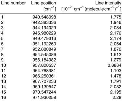
to determine the spectral calibration parameters from in-flight measurements, because they are not stable enough in time to be determined from lab measurements on ground. The parameters are derived from atmospheric limb or deep space measurements taken with the chemistry mode spectral resolution (i.e. an MOPD of_±8 cm), using selected CO2 lines with well-known spectral positions in the spectral range between 940 and

20

980 cm−1_{(see Table 1). These lines are measured during flight with a relatively good} signal-to-noise ratio, they are well isolated over a large altitude range and are globally available.

The spectral calibration parameters are deduced from a set of radiometrically cali-brated spectra. For the generation of this dataset, a first guess for the laser wavelength

(15)

AMTD

7, 2827–2878, 2014

GLORIA

A. Kleinert et al.

Title Page

Tables Figures

◭ ◮

Back Close

Full Screen / Esc

Discussion

P

a

per

|

D

iscussion

P

a

per

|

Discussion

P

a

per

|

Discuss

ion

P

a

per

|

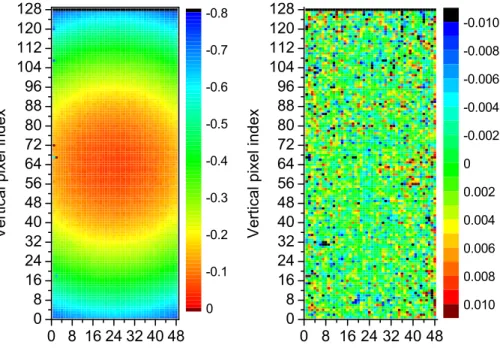
is used, and the oﬀ-axis eﬀect is not taken into account. In this dataset, the position of a certain spectral line moves to smaller wavenumbers for pixels that are farther away from the optical axis (Eq. 11). For each of the CO2lines listed in Table 1, the apparent

line position is evaluated for each pixel. The interferogram is strongly zerofilled, such that the spectrum is sampled on a fine grid, about two orders of magnitude finer than

5

the original grid. The abscissa value of the line maximum of the oversampled spectrum is taken as line position. The line position across the detector array gives a two dimen-sional bell shaped curve (Fig. 5, left). The position of the optical axis on the detector array is given by the maximum of this curve. A second order 2-D polynomial, which is a good approximation to the cosine dependency of the values, is fitted to the data and

10

the maximum of the fitted curve is taken as optical axis position.

Once the optical axis position is known, the distancer_i_,_j of each pixel centre from the optical axis is calculated, and the line position found for each pixel is expressed as a function of this distance. Using Eqs. (11) and (12) and rearranging the terms, we get:

σ_i2_,_j = b

2

b2₊_r2

i,j

σ₀2 (13)

15

A curve fit of the form

y= a0

a₀+xa1 (14)

gives the fit results forb=√a₀and forσ₀=√a₁. The actual laser wavelength is

calcu-20

lated from the deviation ofσ₀to the true line position of the respective line as given in the HITRAN database (Rothman et al., 2009):

λ_laser=λ_apriori_×σ0

σ_H (15)

whereλ_laser is the laser wavelength, λ_apriori is the first guess of the laser wavelength

25

(16)

AMTD

7, 2827–2878, 2014

GLORIA

A. Kleinert et al.

Title Page

Tables Figures

◭ ◮

Back Close

Full Screen / Esc

Discussion

P

a

per

|

D

iscussion

P

a

per

|

Discussion

P

a

per

|

Discuss

ion

P

a

per

|

as derived from the measurement, andσ_H is the true line position from the HITRAN database.

The fit of the spectral calibration parameters is done separately for each of the lines listed in Table 1. The mean values over all spectral lines are used for spectral cali-bration. Figure 5 shows the determined line position for the CO2 line at 951.19 cm−

1

5

across the detector array before (left) and after spectral calibration (right) from a deep space measurement. While the bell shape is clearly visible in the left plot, the right plot does not show any systematic line position variation across the array. The pixel to pixel variation of the line position comes from the noise in the line position determination method.

10

5 Data processing

The level 0 to 1 processing transforms the measured raw interferograms into radiomet-rically and spectrally calibrated spectra. The core of the level 0 processing is the resam-pling of the interferograms. The raw interferograms are sampled on a time-equidistant grid. Before Fourier transform, they have to be interpolated onto a space-equidistant

15

grid, taking velocity variations of the interferometer drive into account. The algorithm used to transfer the interferogram from the time domain into the spatial domain is an approximate Whittaker–Shannon interpolation (Shannon, 1949) as proposed by Brault (1996). The level 0 processing also includes a quality check of the data, spike detec-tion and correcdetec-tion, non-linearity correcdetec-tion, correcdetec-tion of phase errors, and the spectral

20

calibration.

The level 1 processing comprises the Fourier transform converting the interfero-grams to complex spectra and the radiometric calibration. During radiometric calibra-tion it has to be considered that the self-emission of components within the instrument is phase-shifted both with respect to the atmospheric signal and among the

compo-25

(17)

AMTD

7, 2827–2878, 2014

GLORIA

A. Kleinert et al.

Title Page

Tables Figures

◭ ◮

Back Close

Full Screen / Esc

Discussion

P

a

per

|

D

iscussion

P

a

per

|

Discussion

P

a

per

|

Discuss

ion

P

a

per

|

perform the calibration completely in the complex domain as proposed by Revercomb et al. (1988). A prerequisite for this approach is that the phase relation between the diﬀerent components is stable between calibration and scene measurements. Phase changes between calibration and scene measurements, which can be characterised (e.g. phase changes due to a shift of the interferogram on the OPD axis) have to be

5

corrected prior to radiometric calibration.

Since the phase is diﬀerent for interferograms measured during forward and back-ward movement of the interferometer slide, the two sweep directions have to be pro-cessed separately.

The level 1 product consists of complex calibrated spectra. When the calibration has

10

been performed correctly, all atmospheric contribution is contained in the real part of the spectrum while the imaginary part contains only noise. The imaginary part serves as quality control and is used to determine the noise equivalent spectral radiance (NESR).

5.1 Level 0 processing

15

5.1.1 Quality control

The time stamps within one cuboid are checked for equidistance. The number of time ticks between two consecutive frames should not differ by more than_±1. Any larger difference points towards lost frames. If a larger difference is detected, the file is dis-carded from further processing.

20

5.1.2 Spike detection and correction

Due to radio frequency interferences produced by external units located outside the GLORIA spectrometer, the serial data link between IR detector frontend electronics and interferometer electronics is sporadically de-synchronised, producing spikes in the interferograms. The immunity against the EMC disturbance depends on the gimbal yaw

(18)

AMTD

7, 2827–2878, 2014

GLORIA

A. Kleinert et al.

Title Page

Tables Figures

◭ ◮

Back Close

Full Screen / Esc

Discussion

P

a

per

|

D

iscussion

P

a

per

|

Discussion

P

a

per

|

Discuss

ion

P

a

per

|

position of the instrument. Especially blackbody measurements, where the instrument looks approximately in flight direction, are affected by spikes. These spikes need to be identified and corrected, as a single spike in the interferogram affects all data points of the spectrum. Two different methods are used to identify the spikes. One method is based on the identification of a specific pattern in affected frames. This method

5

identifies spikes independently of the measurement type and the spike intensity. The second method is statistical and allows to identify single large spikes that do not show the specific frame pattern.

If a frame is aﬀected by spikes, the distribution of the aﬀected pixels usually shows a specific pattern. In case of a spike several pixels in a region show exactly the same

10

value. In nominal measurements the probability that neighbouring pixel show the same value is very low because of measurement noise and diﬀerent sensitivity properties of each pixel. The strategy for searching spikes is a loop over all pixels in each frame. If at least one horizontal neighbour of a pixel has the same value as the pixel itself, a pixel is marked as spike candidate. A spike event is detected, when at least for two rows the

15

number of spike candidates per row passes an empirical threshold.

Manual inspection has shown that about 90 % of all spike events exhibit the pattern and are thus detected by this method. But if only one or few pixels are aﬀected, this method fails. A second method, which does not use the characteristic pattern, is there-fore applied to the data. For this method, all interferograms x_i are normalised to the

20

same scale with

ˆ

x_i =xi−xi

σ_i , (16)

wherex_i andσ_i are the mean and standard deviation of theith interferogram. The nor-malisation compensates for diﬀerent sensitivities of the individual pixels. After

normali-25

(19)

AMTD

7, 2827–2878, 2014

GLORIA

A. Kleinert et al.

Title Page

Tables Figures

◭ ◮

Back Close

Full Screen / Esc

Discussion

P

a

per

|

D

iscussion

P

a

per

|

Discussion

P

a

per

|

Discuss

ion

P

a

per

|

flagged as spike contaminated. Pixels with values deviating by more than three times the current standard deviation from the frame mean are then flagged as spiked. Close to the ZOPD the variation from frame to frame is generally high, therefore a region of ±0.06 cm around the peak is excluded from this method.

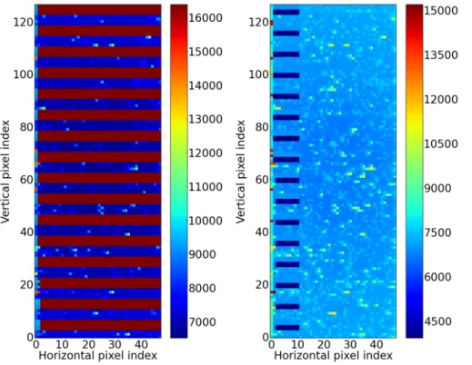
Figure 6 shows two examples of frames aﬀected by spikes with the typical pattern

5

which is identified by the first method. In the left picture, the affected pixels show the maximum value of 16 383 and nearly all columns are affected, whereas in the right picture, only few columns in the left part of the picture are affected, and the values of the affected pixels (light blue for the upper two and dark blue for the lower two rows of each affected block) are only slightly different from the values of the non-affected pixels,

10

leading to spikes with small amplitudes. Figure 7 shows the normalised mean (top) and standard deviation (bottom) of a raw interferogram of an atmospheric measurement as calculated following the second method. The green curve shows three times the standard deviation. The red crosses mark identified spikes.

Detected spikes are corrected by replacing the spike with the mean value of the

15

neighbouring frames. This correction method does not work for spikes close to the ZOPD (_±0.02 cm). If a spike is detected in this range, the measurement is discarded. Outside the range close to the ZOPD, the eﬀect of the corrected spike on the spectrum is well below noise level and the interferogram can be used.

5.1.3 Non-linearity correction

20

The non-linearity correction is performed by assigning to each interferogram value the value that would have been measured with a linear detector system (see Sect. 3.2).

5.1.4 Abscissa determination

In principle, the abscissa in the space domain can be chosen freely. Ideally, the sam-pling is chosen such that it corresponds to the measurement samsam-pling in the time

(20)

AMTD

7, 2827–2878, 2014

GLORIA

A. Kleinert et al.

Title Page

Tables Figures

◭ ◮

Back Close

Full Screen / Esc

Discussion

P

a

per

|

D

iscussion

P

a

per

|

Discussion

P

a

per

|

Discuss

ion

P

a

per

|

domain:

∆x=v_×∆t (17)

∆_x _{is the sampling in the space domain,} _v _{is the mean velocity and} ∆_t _{is the}

sam-pling in the time domain. For the current flight configuration of GLORIA with a mean

5

velocity of 1.27 cm s−1 and a sampling frequency of 6281 Hz, the natural sampling in the space domain as calculated from Eq. (17) would be 2.04 µm. A sampling denser than the natural sampling increases the number of points without adding new informa-tion, whereas a coarser sampling reduces the spectral bandwidth, leading to aliasing eﬀects if out-of-band signals are not filtered. For an optimised processing (see Sect. 6)

10

it is furthermore desired that the sampling distance is a multiple of 10−4nm and that the MOPD is hit by a sampling point. The sampling grid in the space domain is chosen as∆x=2 µm, which is slightly smaller than the natural sampling of 2.04 µm.

5.1.5 Phase correction

Using the complex calibration approach proposed by Revercomb et al. (1988), no

ex-15

plicit phase correction needs to be performed. It must be ensured, however, that the instrumental phase is the same for calibration and scene measurements, such that any instrument contribution cancels out during calibration. This implies, that the ZOPD po-sitions of the diﬀerent interferograms are perfectly overlying. A shift in the interferogram domain corresponds to a linear phase change in the spectral domain. Such a shift can

20

be caused by fringe count errors (FCEs), where the laser fringes are not counted prop-erly during turnaround, leading to a wrong starting point of the data acquisition. A drift of the reference laser wavelength may also lead to a shift of the ZOPD position. These eﬀects are pixel independent, therefore it is suﬃcient to determine the shift between interferograms (or the linear phase change in the spectral domain) for a single pixel. In

25

(21)

AMTD

7, 2827–2878, 2014

GLORIA

A. Kleinert et al.

Title Page

Tables Figures

◭ ◮

Back Close

Full Screen / Esc

Discussion

P

a

per

|

D

iscussion

P

a

per

|

Discussion

P

a

per

|

Discuss

ion

P

a

per

|

In emission FTS, the calculated phase of the complex spectrum is strongly varying with the signal from the atmosphere, because instrument contributions, which are out of phase, are in the same order of magnitude as the atmospheric signal (Revercomb et al., 1988; Kleinert and Trieschmann, 2007). Figure 8 shows the real part of an un-calibrated but phase corrected blackbody spectrum (top), the real part of a deep space

5

spectrum (middle) and the imaginary part of a deep space spectrum (bottom). In case of the blackbody spectrum, the instrument contributions are negligible for the phase calculation, because the signal coming from the source is one order of magnitude larger than the radiation emitted from the instrument. The calculated phase reflects the instrumental properties (e.g. dispersion of the beamsplitter) which vary slowly with

10

wavenumber (Fig. 9, black curve). In case of the deep space spectrum, the situation is diﬀerent. The instrument baseline is negative in a wide spectral range, and the beam-splitter emission, which is found in the imaginary part, gives a considerable contribution around 800 cm−1

. Therefore the phase angle changes rapidly with wavenumber, reflect-ing more the atmospheric spectrum than the instrumental phase (Fig. 9, red curve). In

15

order to identify a linear phase change between diﬀerent measurements, a spectral region has to be used where the contribution from the source is strong compared to the instrument self emission for all types of measurement. In case of GLORIA, the spectral range between 1025 and 1060 cm−1is best suited for this purpose, because in this range the atmospheric signal is high due to the strong ozone signature, while

20

instrument contributions are comparably low. As seen in Fig. 9, the phase in that range is the same as for the blackbody measurement.

The phase, which is calculated for a reference interferogram (usually a blackbody interferogram), is called the standard phase. For each interferogram, the diﬀerence to the standard phase is calculated, and a linear fit is applied in the range between 1010

25

(22)

AMTD

7, 2827–2878, 2014

GLORIA

A. Kleinert et al.

Title Page

Tables Figures

◭ ◮

Back Close

Full Screen / Esc

Discussion

P

a

per

|

D

iscussion

P

a

per

|

Discussion

P

a

per

|

Discuss

ion

P

a

per

|

The slope directly gives the shift in the interferogram domain. The shift is subtracted from the abscissa determined above.

5.1.6 Delay

The time stamps of the infrared data exhibit a certain delay with respect to the reference laser data. This is due to diﬀerent signal travelling times in the electronics as well as

5

the finite integration time. The delayt_delay is given as:

t_delay= 1 f_frame−

1

2tint+treset

−t_L (18)

f_frame is the frame frequency, t_int the integration time, t_reset is the reset time for the integration capacitor of the detector, andt_Lis the runtime of the reference laser signal.

10

The frame frequency and the reset time are dependent on the used array size. The delay is calculated for the centre of the integration interval.

The delay is corrected by subtracting the delay time from the time stamps of the infrared signal.

5.1.7 Spectral calibration

15

The correct assignment of the spectral axis for a pixel on the optical axis is ensured through the use of the correct laser wavelength when building the space axis from the reference laser data. The laser wavelength is one of the spectral calibration parameters determined from selected atmospheric or deep space measurements.

In order to obtain the same abscissa for all pixels, the abscissa of each interferogram

20

(23)

AMTD

7, 2827–2878, 2014

GLORIA

A. Kleinert et al.

Title Page

Tables Figures

◭ ◮

Back Close

Full Screen / Esc

Discussion

P

a

per

|

D

iscussion

P

a

per

|

Discussion

P

a

per

|

Discuss

ion

P

a

per

|

5.1.8 Interferogram resampling

Once the desired abscissa in space is defined, the interpolation points in time are calculated from the time-space-relation given by the reference laser. Linear interpola-tion between adjacent points is suﬃcient to calculate the time for the desired point in space. The actual resampling is done by convolving the measured interferogram with

5

an apodised sinc kernel. The output of the level 0 processor consists of data cuboids containing non-linearity corrected, spectrally calibrated interferograms that are sam-pled on a space-equidistant grid.

5.2 Level 1 processing

The level 1 processing comprises the Fourier transform of the interferograms and the

10

complex radiometric calibration.

5.2.1 Fourier transform

The Fourier transform calculates complex spectra from the resampled interferograms. In the standard processing, the interferograms are multiplied by the Norton–Beer-strong apodisation function (Norton and Beer, 1976, 1977), since apodised spectra

15

are used for the temperature and trace gas retrieval.

5.2.2 Radiometric calibration

Radiometrically calibrated spectra are obtained by dividing the atmospheric spectrum by the gain and subtracting the oﬀset following Eq. (3). Gain and oﬀset are drifting in time, therefore they are interpolated linearly between two calibration sequences to the

20

time of the atmospheric measurement.

(24)

AMTD

7, 2827–2878, 2014

GLORIA

A. Kleinert et al.

Title Page

Tables Figures

◭ ◮

Back Close

Full Screen / Esc

Discussion

P

a

per

|

D

iscussion

P

a

per

|

Discussion

P

a

per

|

Discuss

ion

P

a

per

|

problem (e.g. pointing variations during interferogram acquisition or severe misalign-ment) or a processing problem (e.g. a phase shift between atmospheric and calibration measurements).

The real part of the calibrated spectrum serves as input to the temperature and trace gas retrieval.

5

6 Processor optimisation

The data processing as described in Sect. 5 has to be performed for each individual pixel, i.e. several thousand times per measurement. Therefore especially time consum-ing operations like the interferogram resamplconsum-ing have to be optimised.

Since the processing is still under development, a two-track strategy is followed: at

10

first, the processing is programmed in IDL (Interactive Data Language), using the her-itage of the processor that was developed for the balloon-borne and airborne MIPAS instruments (Friedl-Vallon et al., 2004; Woiwode et al., 2012). The IDL processor with the character of a prototype allows for diagnostics, visualisation etc. and is easy to modify for testing purposes. It is used for quality control of the data, the definition of

15

the abscissa and the linear phase correction or interferogram shift. These processing steps need to be done only for one or few pixels per measurement. The computation-ally expensive resampling of the interferograms, which has to be done for each pixel individually, is encapsulated in a stand-alone C programme, which also performs the non-linearity correction and spectral calibration and takes the externally computed

de-20

lay and phase correction into account.

In view of a raw data rate of 73.6 MiB s−1, the processor has to be optimised in order to approach or possibly even exceed the data acquisition speed. This is especially important for possible future long-duration balloon or satellite missions where it is not possible to store all the raw data. Then on-board processing may become necessary

25

(25)

AMTD

7, 2827–2878, 2014

GLORIA

A. Kleinert et al.

Title Page

Tables Figures

◭ ◮

Back Close

Full Screen / Esc

Discussion

P

a

per

|

D

iscussion

P

a

per

|

Discussion

P

a

per

|

Discuss

ion

P

a

per

|

6.1 Description of the operational level 0 processor

Mathematically, the interpolation corresponds to a convolution of each pixel’s interfero-gram data with a sinc function. This is implemented in the level 0 processor using a set of finite-width convolution kernels. For the sake of computing performance optimisa-tion, each kernel consists of only 16 data points. The convolution kernel is apodised

5

using a Kaiser filter in order to suppress the Gibbs oscillation. The diﬀerent samplings of the convolution kernel are pre-tabulated to avoid computationally expensive runtime calculations of the sinc values. In order to reduce the size of the whole lookup-table, the kernel values are stored in an integer (i.e. fixed point) representation. For each sample on the target axis, the correct kernel is chosen from the table depending on the

10

position of the new sampling point.

Due to the eﬀect of cache misses, a prerequisite for the eﬃcient convolution of the data is that the interferograms be contiguous in memory. Unfortunately, due to the na-ture of the data acquisition, the input is strucna-tured in a transposed form. The transposi-tion of the input data is therefore the first processing step, followed by the interpolatransposi-tion

15

setup and, finally, the convolution itself.

To avoid nonlinear memory access, a data structure has been specifically designed which maps each point of the pre-defined output abscissa to the correct input data and convolution kernel.

To ensure performance and compatibility, the level 0 processor is written in the C

20

programming language. On top of the core processor, a Python interface has been added for more eﬃcient interoperability with other processing steps.

6.2 Performance

The runtime of the level 0 processor is, apart from file input/output, dominated by two calculations. The first is the transposition of the measured image, the second is the

25

(26)

AMTD

7, 2827–2878, 2014

GLORIA

A. Kleinert et al.

Title Page

Tables Figures

◭ ◮

Back Close

Full Screen / Esc

Discussion

P

a

per

|

D

iscussion

P

a

per

|

Discussion

P

a

per

|

Discuss

ion

P

a

per

|

Initial optimisation targets were found by analysing both algorithms. Fortunately, both are by their nature very well suited for shared-memory parallelisation, which has been realised using the OpenMP protocol. Further potential for optimisation was discovered by analysing the assembly code generated by the C compiler. Using the SSE instruction set, the vector registers of modern CPUs could be used for optimised

reimplementa-5

tions of both the cuboid transposition and resampling.

Both approaches, parallelisation and vectorisation, were combined and resulted in a high-performance system able to match and exceed the data rate of the instrument. All following runtime measurements have been performed using a single GLORIA chemistry mode measurement. The cuboid file in question is about 945 MiB1 in size

10

and took 12.8 s to record. The CPU of the benchmark computer was an AMD Opteron 6128 with 8 cores clocked at 2000 MHz. In order to eliminate the impact of disk I/O, the relevant files have been read from and written to memory using tmpfs, a RAM-based file system for Linux.

Figures 10 and 11 show the runtimes and speedup factors for the convolution, the

15

cuboid transposition and the total processing for the non-vectorised and the vectorised implementations, respectively. The non-vectorised version takes about 56.4 s to run without parallelisation, which is reduced to 12.4 s using 8 concurrent threads. Note that this already slightly exceeds the real-time speed target. With the vectorisation (SSE) these timings reduce further to 36.9 s (single-thread) and 9.5 s (8 threads), respectively.

20

The most eﬃciently parallelised algorithm is by far the convolution, whose speedup scales almost linearly with the number of threads employed. The cuboid transposition involves a larger non-parallel overhead, making it scale less ideally. The use of SSE instructions mitigates the benefits of parallelisation only slightly, so that using both in conjunction is very eﬀective.

25

The cuboid transposition benefits most from vectorisation with relative speedups larger than 4 in single-thread and still larger than 3 in 8-thread mode. The speedup is expected to become less prominent when more threads are used concurrently because

1

(27)

AMTD

7, 2827–2878, 2014

GLORIA

A. Kleinert et al.

Title Page

Tables Figures

◭ ◮

Back Close

Full Screen / Esc

Discussion

P

a

per

|

D

iscussion

P

a

per

|

Discussion

P

a

per

|

Discuss

ion

P

a

per

|

memory bandwidth remains limited. In contrast, the speedup for the convolution is al-most constant at 25 %, while the processor as a whole runs between 31 % and 54 % faster with SSE enabled.

In total, the C code with all its optimisations is more than two orders of magnitude faster than our IDL prototype.

5

6.3 Outlook

Aside from x86-64, other computational architectures have been considered. Prelim-inary implementations of the level 0 processor on NVIDIA GPUs have been tested, but resulted in only a small overall performance gain of about 5 % compared with the CPU version. A more detailed study revealed that only 33 % of the GPU processing

10

time was used for the computations, i.e. the transfer of the large data volumes between system and graphics memory resulted in a bottleneck. In the future, an implementa-tion on a shared-memory CPU/GPU system such as the AMD Fusion platform may be investigated for better results.

The current level 1 processing uses the IDL routines developed for MIPAS with slight

15

modifications. In the long run, this software is too ineﬃcient for use with large volumes of GLORIA data and the degree of automation is limited. An integrated level 0 to 1 processing suite, which is implemented mainly in the Python programming language and includes optimisations for performance-critical sections, is under development.

7 Results

20

(28)

AMTD

7, 2827–2878, 2014

GLORIA

A. Kleinert et al.

Title Page

Tables Figures

◭ ◮

Back Close

Full Screen / Esc

Discussion

P

a

per

|

D

iscussion

P

a

per

|

Discussion

P

a

per

|

Discuss

ion

P

a

per

|

7.1 Radiometric accuracy

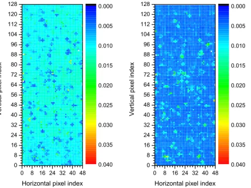
An estimate for the radiometric accuracy can be achieved by analysing the calibrated spectra of the hot blackbody measurements. Since the data of the hot blackbody are not used for calibration in the current calibration approach, they provide independent measurements from a known source.

5

Figure 13, left, shows the mean relative radiance error in the spectral range from 900 to 950 cm−1_{for each pixel, calculated from one calibration sequence of the HALO} flight on 26 September 2012. Black and brown pixels exhibit an error of more than ±1.5 %. If a threshold of 1.5 % is applied to the data, less than 10 % of the pixels have to be discarded. This threshold provides a good compromise between the accuracy

10

requirement of 1 to 2 % and the number of discarded pixels. Besides the outliers, the calibrated blackbody data show a positive bias of less than 1 % which is strongest in the middle of the detector. Such a bias can be evoked by temperature inhomogeneities of the blackbody surface. Currently the mean over five temperature sensors across the blackbody area is taken as blackbody temperature for all pixels, although the sensors

15

show a temperature variation of approximately 0.3 K across the surface. This error is currently considered acceptable, but investigations are under way how the radiomet-ric accuracy can be improved by taking the temperature inhomogeneity into account. Furthermore, the temperature homogeneity will be improved for future flights through improvements of the thermal control software and the operation procedures.

20

Drift of radiometric gain and offset

The drifts of the radiometric gain and offset are evaluated for the HALO flight on 13 September 2012. For the evaluation of the drift, a mean gain and offset function over the whole detector array is calculated for each calibration sequence. Then the mean gain and offset over all calibration sequences is calculated, and for each calibration

25

(29)

AMTD

7, 2827–2878, 2014

GLORIA

A. Kleinert et al.

Title Page

Tables Figures

◭ ◮

Back Close

Full Screen / Esc

Discussion

P

a

per

|

D

iscussion

P

a

per

|

Discussion

P

a

per

|

Discuss

ion

P

a

per

|

it shows the relative deviation from the mean for each calibration sequence. The gain function varies by less than_±2 % over the nominal spectral range, showing that the calibration frequency is suﬃciently high for the gain determination. Problems in the baseline determination around the strong ozone band at 1040 cm−1 (see Sect. 3.3) also aﬀect the gain function in this range.

5

Figure 15 shows the offset, representing the instrument self emission. The offset is negative, because instrument contributions having a phase ofπwith respect to the in-coming radiance are stronger than instrument contributions which are in phase with the incoming radiance. The lower panel shows the difference from the mean spectrum for each calibration sequence. The drift above 900 cm−1 is governed by the temperature

10

drift of the instrument. This drift can be captured well by the linear interpolation of the oﬀset. The spectral feature below 900 cm−1 stems from the bulk emission of the ger-manium entrance window. The intensity of this feature is governed by the temperature of the entrance window, which changes faster than the instrument temperature. In this region a simple linear interpolation of the calibration measurements may be insuﬃcient.

15

Further characterisation work is planned in order to improve the radiometric calibration in this spectral range.

7.2 Spectral calibration accuracy

The accuracy of the spectral calibration is estimated by determining the line positions of selected lines after spectral calibration and comparing the values to the ones given

20

in the HITRAN database. In order to enhance the signal-to-noise ratio, 48_×8 pixels (horizontal_×vertical) are co-added, such that the co-added data form an array of 1_×16 super-pixels. For each of these super-pixels, the line positions of the 16 CO2 lines

listed in Table 1 as well as of two H₂O lines at 1395.8 and 1399.2 cm−1 have been determined. The relative line position error expressed in ppm is shown in Fig. 16. The

25

line indices 1 to 16 correspond to the ones given in Table 1, the line indices 17 and 18 correspond to the two H2O lines named above. For the CO2lines the line position