2Physics Department, University of Crete, Heraklion, Greece
3Department of Electrical and Computer Engineering, Miami University, Oxford, OH, USA 4Institute of Space and Atmospheric Studies, University of Saskatchewan, Canada
Received: 15 October 2008 – Revised: 26 January 2009 – Accepted: 30 January 2009 – Published: 2 March 2009
Abstract. Sporadic E layers (Es) follow regular daily
pat-terns in variability and altitude descent, which are deter-mined primarily by the vertical tidal wind shears in the lower thermosphere. In the present study a large set of sporadic E layer incoherent scatter radar (ISR) measurements are an-alyzed. These were made at Arecibo (Geog. Lat.∼18◦N; Magnetic Dip∼50◦) over many years with ISR runs last-ing from several hours to several days, coverlast-ing evenly all seasons. A new methodology is applied, in which both weak and strong layers are clearly traced by using the vertical elec-tron density gradient as a function of altitude and time. Tak-ing a time base equal to the 24-h local day, statistics were obtained on the seasonal behavior of the diurnal and semid-iurnal tidal variability and altitude descent patterns of spo-radic E at Arecibo. The diurnal tide, most likely the S(1,1) tide with a vertical wavelength around 25 km, controls fully the formation and descent of the metallicEs layers at low
altitudes below 110 km. At higher altitudes, there are two prevailing layers formed presumably by vertical wind shears associated mainly with semidiurnal tides. These include: 1) a daytime layer starting at∼130 km around midday and de-scending down to 105 km by local midnight, and 2) a less frequent and weaker nighttime layer which starts prior to midnight at∼130 km, descending downwards at somewhat faster rate to reach 110 km by sunrise. The diurnal and semidiurnal-like pattern prevails, with some differences, in all seasons. The differences in occurrence, strength and de-scending speeds between the daytime and nighttime upper layers are not well understood from the present data alone and require further study.
Correspondence to:N. Christakis (nchristakis@tem.uoc.gr)
Keywords. Ionosphere (Ionosphere-atmosphere
interac-tions; Mid-latitude ionosphere) – Radio science (Ionospheric physics)
1 Introduction
Incoherent scatter radar (ISR) and ionosonde studies show that mid- and low-latitude sporadic E is not as “sporadic” as its name implies but a regularly occurring phenomenon at low mid-latitudes. There is a repeatability inEs layer
occur-rence and altitude descent that is attributed to the global sys-tem of the tidal winds in the lower thermosphere. As shown by Mathews (1998) in his review paper, the Arecibo ISR ob-servations revealed a fundamental role played by the diurnal and semidiurnal tides in the formation and descent of spo-radic E layers, which often are also referred to as “tidal ion layers” (TILs). The 12- and 24-h tidal effects onEs
forma-tion have been recognized also in ionosonde observaforma-tions at midlatitudes (see e.g. Haldoupis et al., 2006, and more refer-ences therein). The connection betweenEs and tides is not
surprising given that the dominant winds in the E-region are the solar tides (Chapman and Lindzen, 1970). These gov-ern the variability and descent of sporadic E through their vertical wind shears, which also move downward following the tidal phase speed propagation. All this is in line with the windshear theory and numerical models (see e.g. White-head, 1989; Carter and Forbes, 1999), which predict metallic ion layer formation at vertical wind shear ion-convergence nodes.
924 N. Christakis et al.: Seasonal variability and descent of sporadic E at Arecibo
(a) (b)
Fig. 1.The Arecibo ISR electron density profile measurements used in the present study:(a)distribution of observation days per month per calendar year over a period of 14 years, and(b)distribution of ISR continuous operation intervals in days.
and importance of the semidiurnal tides on the formation and descent ofEs. Questions also exist with respect to the
con-fluence of the various tidal modes, as well as their overall dominant features, which if they can be defined then could be implemented in large-scale atmosphere-ionosphere mod-els. Moreover, there are questions about the tidal effects on basicEsproperties, such as the diurnal and seasonal
variabil-ity of the layers, which are still not well understood. The purpose of the present work is to provide more in-sight into the nature of sporadic E tidal variability and layer descent. To achieve this objective, we use an extended set of incoherent scatter radar (ISR) electron density observa-tions made at Arecibo over many years with radar runs last-ing from several hours to several days with a reasonably good seasonal coverage. Furthermore, in the present work a new method to analyze the sporadic E layer ISR radar measure-ments is applied, in which, instead of using the measured electron density as a function of altitude and time to trace the layers, we use the vertical electron density gradientdNe/dz.
The logarithm of this quantity turns out to be a sensitive pa-rameter in tracing the altitudinal layer structure and in iden-tifying well both strong and weak layers in altitude as a func-tion of time. Recent works using the Arecibo ISR to study Es ion layers, neutral metal layers in the lowest E-region, as
well as the upperE region intermediate descent layers in-clude those by Zhou et al. (2005, 2008), Earle et al. (2000), Bishop et al. (2002) and Bishop and Earle (2003).
In the present paper we concentrate on the mean seasonal behavior of sporadic E in terms of its tidal variability. To our knowledge, this is the first statistical study on Es done by
means of using ISR measurements. Also we infer from the data typical tidal wave parameters, especially with regards to the diurnal tide, which dominates thermospheric heights below 110 km at low latitudes, and use a simple model to
exemplify the tidal effects onEsaltitude descent versus local
day time.
2 Data and method of analysis
The ISR at Arecibo (Geog. Lat.∼18◦N; Geom. Lat.∼30◦N)
is the best instrument available to monitor the ionospheric structure with superb sensitivity and good range and time resolution. Among various ionospheric phenomena, the Arecibo radar is particularly suited for investigating the al-titudinal structure and dynamics of narrow sporadic E layers. Contrary to previous AreciboEs studies which were based
on radar runs of a few days, statistical estimates are obtained here for the first time by using a large set of measurements. These comprise about 140 days of radar observations dis-tributed over all seasons, made over a period of 14 years from 1986 to 2000 (for details on the radar operation mode see Zhou, 1998). In the present analysis, electron density pro-files measured between 60 and 480 km with 600 m altitude resolution integrated over times of a few seconds are ana-lyzed. The individual observational periods range from part of a day to 8 days. The histograms in Fig. 1 summarize the monthly observations distributed over a calendar year and the duration in days of continuous radar observations. As seen, the observing periods are distributed fairly evenly over the year, whereas the average continuous radar run duration is
∼2.3 days.
Since the efforts here focus on studying the tidal variabil-ity of sporadic E in altitude and time and not their strength in terms of electron density, a novel method is introduced for analysis, which makes use of the electron density gra-dient log(dNe/dz), instead of logNe to produce
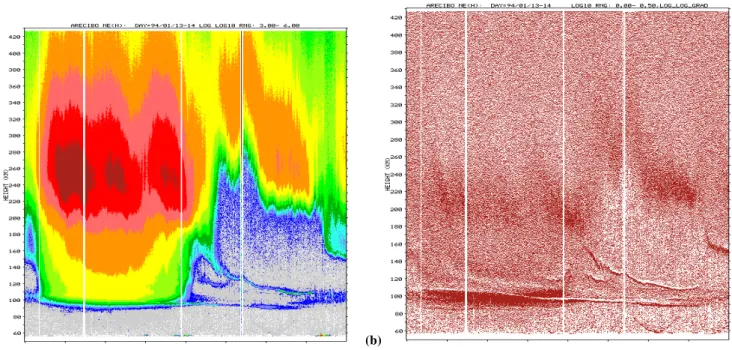
(a)
(b)
Fig. 2. Example of different presentation of the measured electron density profiles by the Arecibo ISR during a period of 24 h starting at 06:00 LT (ordinate axis). The left panel is the usual logNeheight-time-intensity (HTI) plot whereas in the right panel is the log(dNe/dz)plot
used for the purposes of the present study.
density gradient). The software developed for this purpose computes HTI plots within a range of heights versus one 24-h local day, c24-hosen wit24-h t24-he purpose of investigating tidal effects on sporadic E. As inferred from Fig. 2, which shows HTI plots for logNeand log(dNe/dz)for a typical day of
ob-servation, the log(dNe/dz)method detects the location of
nar-row sporadic E layers rather accurately, thus it is rather suit-able for studying the layer tidal variability and descent with time.
Data from approximately 140 days over a period of 14 years have been gathered and analyzed. Examples of typical log(dNe/dz) HTI plots are presented in Fig. 3 for two
differ-ent periods of two consecutive days. The dominant features and complexity of the layering structures are well depicted. The available data were separated according to season and the traces were first classified in identifiable groups and then digitized manually with the aid of GetData-Graph Digitizer (Fedorov, 2008) software. Careful inspection of the entire number of the HTI plots led to identification of 3 main groups of layers, a diurnal trace at lower altitudes below 110 km and two upper layers, a daytime and a nighttime one. The traces of every available day (or fragment of day) were output as mean hourly samples over a 24-h day. The analysis included only those traces which could be clearly seen in the HTI plots for at least part of one hour and could be identified as part of an ongoing layer structure. For instance, at the top left panel of Fig. 3 the small trace at 120 km between 02:00 h and 03:00 h local time (LT) was not considered, since it could not be clearly identified as part of a persisting layer. Next, the
dominant traces were averaged for every one of the four sea-sons.
3 Presentation of results
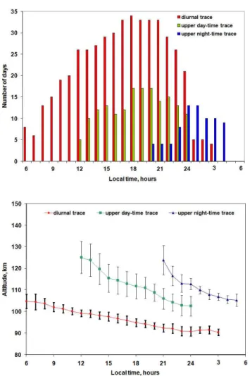
The statistics of the main sporadic E layers with altitude and local time during a 24-h day period are summarized in the following 4 figures for the seasons of winter (Fig. 4), spring (Fig. 5), summer (Fig. 6) and fall (Fig. 7). Each figure has two parts: 1) the upper panel containing histograms of the hourly samples available for all the identified groups of lay-ers present in the HTI plots, thus indicating the relative oc-currence of each group, and 2) the lower panel showing the mean location of the corresponding layers plotted in altitude versus local time for the 24-h day period starting at 06:00 LT. The information in the two panels is color-coded for iden-tification, whereas the error bars in the lower panel are the mean deviation from the mean, representing the variability in the layer’s altitude location at a given local time.
926 N. Christakis et al.: Seasonal variability and descent of sporadic E at Arecibo
Fig. 3.Typical log(dNe/dz)HTI plots used in the present study for identifying the differentEslayers prevailing in the Arecibo data. These
traces were first grouped and then digitized, so they could be statistically analyzed for every season.
relate to the diurnal tide, and two upper altitude traces refer-ring to a daytime and a nighttime descending layer, spaced about 10 to 12 h apart, apparently being controlled mainly by the semidiurnal tide.
The diurnal trace sets in at sunrise somewhat below 110 km, while the semidiurnal-like ones prevailing at higher altitudes start at about 130 km a couple of hours prior to local noon and midnight, respectively. Downward speeds are clearly larger for the semi-diurnally forced layers, which gradually move down and merge with, or taken over by, the slowly descending diurnal layer below. The dominant fea-ture in the data is the diurnal tidal trace which descends from about 106 km down to∼90 km over a period of 24 h. During
summer however, a weaker upper diurnal-like trace is also present at times, starting at about 120 to 125 km to descend with approximately the same speed as the dominant diurnal trace below. This might be regarded as evidence that the diur-nal tide starts higher up in the summer than in other seasons. As seen from the histograms in Figs. 4 to 7, the semidiurnal-like upper traces are less frequent than the pre-vailing diurnal trace at lower altitudes. In addition, the day-time layer is better defined and more frequent than the night-time one. The evidence shows that both connect higher up with the so called intermediate descending layers (IDL) which are broader and weaker but commonly present in the AreciboNeprofiles (see e.g. Mathews, 1998, and references
therein). On the average, the daytime layer appears a cou-ple of hours prior to midday at about 130 km and moves down to∼105 km by midnight with decreasing speeds from ∼3.5 to 2.5 km/h. The less frequent and intermittent
night-time layer appears at∼130 km near 22:00 LT, moving down
to∼110 km by 06:00 LT with average speeds ranging from ∼4.0 to 3.0 km/h. Finally, the trace altitudinal variability,
signified by the error bars in the lower panels of Figs. 4 to 7, can be attributed to various reasons. A likely one is the mod-ulation of tides by planetary waves in the mesosphere. This was proposed by Pancheva et al. (2003) as the mechanism behind the PW-like variability of sporadic E layers. Another possibility is the confluence in forming a layer of more than one tidal modes at a given time and/or contributions from gravity waves.
Figure 8 offers a visual comparison of the statistical results for all four seasons by superimposing the observed mean traces for the lower altitude diurnal ion layer and the upper altitude semidiurnal ones. As seen, on the average there are some discrepancies with seasons, in both altitude and overall variability, which may or may not be significant. The sea-sonal differences are smaller for the low altitude dominant diurnal trace (or layer) for which there is a larger statistical sample. For all practical purposes, the diurnal traces appear to be about the same for all seasons, having relative differ-ences between seasons of∼5 to 7%. It can be argued that
Fig. 4.Statistics of the averagedEstraces as a function of altitude
and local time, during a 24-h day starting at 06:00 LT, shown here for winter (December, January, and February). The upper panel presents the occurrence distributions of the three dominant traces shown separately in the lower panel. The error bars represent the mean error. The colors between the two panels are in correspon-dence.
4 Tidal wavelength estimates and numerical simulation
According to the windshear theory (see e.g. Chimonas and Axford, 1968), a layer remains at the shear convergence null only if it forms fast relative to the time needed for the null to propagate downwards (with the phase velocity of the tidal wave) a distance equal to the layer width. For a given tidal mode, the layer can descend with the vertical tidal phase speed at higher E-region altitudes where the ion-neutral col-lisional control on ion convergence is small. As discussed by Haldoupis et al. (2006), at lower altitudes, the increased number of collisions slows down the vertical descent of the layers because these cannot form fast enough to remain at the convergence null. Thus, they lag behind and descend at
in-Fig. 5.Same as in Fig. 4 but for spring (March, April, May).
creasingly smaller rates with decreasing altitude as compared to the vertical phase velocity of the tide. This is more likely to occur for the case of the semidiurnal tides than the diurnal ones, since the former phase-propagate downwards faster. As a result of ion-neutral collisional forcing, and in line with the-ory and observations, a descendingEstrace can have a fairly
constant slope at upper heights in the altitude versus time frame, which decreases steadily as the layer moves down where ion-neutral collisions become increasingly frequent. Based on this picture, a nearly constant slope at upper heights for theEs trace may provide a good estimate of the
down-ward tidal phase speed.
By considering these facts, Es layer descending speeds
928 N. Christakis et al.: Seasonal variability and descent of sporadic E at Arecibo
Summer
Fig. 6.Same as in Fig. 4 but for summer (June, July, August). See also text for more details.
sporadic E traces, are listed in Table 1. The phase speeds here correspond to the upper heights of the mean traces shown in Figs. 4 to 7, for which the slope computed for consecutive points remains fairly constant (within 10 to 15%). We stress, however, that the computed values are likely to be underesti-mates of the real vertical phase velocities and wavelengths of the tides involved, since ion-neutral collisions are expected to have always some effect for the heights under consideration, that is, below 130 km.
Based on Table 1, the overall mean velocities and wave-lengths plus their mean errors inferred for the different Es
traces are as follows: a) 1.0±0.9 km/h and 25.5±2.1 km for the diurnal trace, b) 3.1±0.8 km/h and 37.1±4.2 km for
the daytime semidiurnal trace, and c) 3.6±0.8 km/h and
43.5±1.6 km for the nighttime semidiurnal trace,
respec-tively. The estimated wavelengths compare well with tidal theory (see e.g. Forbes, 1995) which predicts: 1) a vertical wavelengthλz=27.9 km for the diurnal tidal mode of S(1,1),
which is dominant in the lower thermosphere below 110 km
Fall
Fig. 7.Same as in Fig. 4 but for fall (September, October, Novem-ber).
at Arecibo latitudes (see e.g. Harper, 1977), and 2) verti-cal wavelengths of 33.4 km and 41.0 km for the S(2,6) and , S(2,5) semidiurnal tides, respectively. This suggests that the diurnal S(1,1) tide is the mode that controls the low altitude diurnalEstrace. On the other hand, the wavelength estimates
for the daytime and nighttime upper layers differ somewhat, and thus, can not be ascertained whether the dominant driv-ing semidiurnal tide is the S(2,6) or S(2,5) mode. Since the daytime trace relies on a larger statistical sample, we suggest that the key semidiurnal tide involved is the S(2,6).
Next follow some numerical simulations of the trajecto-ries of the main layers, using the methodology introduced first by Chimonas and Axford (1968) and applied later by Mathews and Bekeny (1978) and more recently by Haldoupis et al. (2006). The simulation was performed separately for the diurnal (lower) and semidiurnal (upper) layers by solving Eq. (1) of Mathews and Bekeny (1978):
w= cosIsinI
1+(νiωi)2
U+(νi
ωi)cosI
1+(νiωi)2
semidiurnal trace
d
λ∼44.4 km
d
λ∼40.8 km
d
λ∼43.2 km
d
λ∼45.5 km
which results from basic windshear theory and gives the ver-tical ion drift velocitywat steady state. Here,U andV are the geomagnetic southward and eastward components of the neutral wind (representing approximately the meridional and zonal wind components, respectively),I is the magnetic dip angle, and (νi/ωi)=ris the ratio of ion-neutral collision
fre-quency to ion gyrofrefre-quency.
Next, Eq. (1) is solved numerically by using a simplified wind system where only a pure tidal zonal wind, either di-urnal or semididi-urnal, is active. The zonal wind profile is de-scribed by the equation:
V =V0exp
z−z
0 2H
cos
2π
λz
(z−z0)+ 2π
T (t−t0)
(2) whereT andλzare the period and vertical wavelength of the
tidal wind,H is a representative scale height for the lower thermosphere between 80 and 150 km,z0is a lower altitude boundary andt0 is a fixed tidal wave phase. For more de-tails regarding the use of this model see Mathews and Bekeny (1978) and Haldoupis et al. (2006).
The values employed for the tidal parameters, in order to describe an S(1,1) tidal mode, were: T=24 h, λz=27.9 km,
V0=110 m/s, z0=73 km, t0=2 h and H=5.5 km. These are similar to those used by Mathews and Bekeny (1978) and Haldoupis et al. (2006) and are consistent with observa-tions of thermospheric tidal winds above Arecibo (Harper, 1977). The shear convergence node was launched at 110 km at 06:00 LT and the trajectory was followed for 24 h. The results of this simulation are shown in Fig. 9 by the solid curve superimposed over the mean diurnalEs traces for all
seasons. As seen, the S(1,1) trajectory produced by the nu-merical model follows closely the observed mean diurnalEs
traces.
On the other hand, shown also in Fig. 9 are simulated traces for the upper altitude daytime and nighttime layers, at-tributed mostly to a semidiurnal tidal action. These curves correspond to S(2,6) with T=12 h, λz=33 km, z0=82 km,
Fig. 8.Superposition of the meanEstraces for the low altitude
diur-nal trace and upper altitude daytime and nighttime semidiurdiur-nal-like traces prevailing in the Arecibo observations for different seasons.
t0=11 h, H=5.5 km and amplitudeV0=80 m/s which is also in line with the findings of Harper (1977). The shear con-vergence node was launched at 140 km at 06:00 LT and this pattern was repeated after 12 h. As seen, the simulated tra-jectories are fairly representative of the observed upper al-titude Es traces, although they do not fit the data so well
930 N. Christakis et al.: Seasonal variability and descent of sporadic E at Arecibo
Fig. 9.Windshear numerical simulation results for a diurnal S(1,1) –λz=27.9 km (lower solid line trace), and a semidiurnal S(2,6) –
λz=33 km (upper solid line traces) zonal tidal wind modes,
super-imposed over the observed meanEstraces presented for all seasons
in Figs. 4 to 7 and Fig. 8. The tidal modes are released near 06:00 LT at 110 km and 140 km for the diurnal and semidiurnal tide, respec-tively. See text for more details.
the upperE region semidiurnal tidal wavelengths increase with altitude, as shown for example by Zhou et al. (2005).
Finally, in the present study we are primarily interested in the layers that showed good continuity. Weak layers be-fore dawn may not be well presented because of the mete-oric interference and production of ionization. The work by Zhou et al. (2005) does not impose any continuity require-ment on the layers. Consequently, they show more layers es-pecially before the dawn hours. Their Fig. 3 indicates a high probability of layer occurrence slightly below 105 km during 02:00–06:00 LT. The altitude and lack of any obvious phase velocity of this layer match well with the model result of the assumed semidiurnal S(2,6) tide shown in Fig. 9. Overall, it thus seems that the simplified wind model used here for sim-ulation supports a consistent physical picture in relation with the formation and descent of sporadic E at low latitudes.
5 Summary and concluding comments
The present analysis allowed for the first time to obtain sea-sonal statistics of sporadic E layer vertical motion and al-titudinal variability as a function of local time at Arecibo (Geog. Lat. 18◦N; magnetic dip∼50◦). The general picture, which is similar for all seasons, is dominated by a diurnal layer at lower altitudes below 110 km and a set of two layers at higher altitudes, a daytime and a nighttime one, that ap-pear to be controlled mainly by semidiurnal tides. Although there are some differences in the descent speed, layer mul-tiplicity and frequency of occurrence, the statistical analysis shows no dramatic changes with season. Regardless of their number density, this is indicative of how regular these layers
appear to be all the time, which may not be surprising, since Arecibo is a low latitude location characterized in general by small seasonal change. We should stress that, although it remains similar, the picture becomes more complex and dy-namic during summer, when sporadic E is known to reach a conspicuous maximum in occurrence and strength (see e.g. recent paper by Haldoupis et al., 2007). In this respect how-ever, the summer differences seen here relative to the rest of the seasons are not drastic and thus, we conclude that they cannot play the decisive role behind the pronouncedEs
sum-mer maximum.
The present results show that on the average, the diurnal tide is the key agent responsible for the formation of strong sporadic E at lower altitudes for all seasons. In their diur-nal course, the layers form, presumably at tidal convergence nulls, near 107 km at∼06:00 LT and move down to altitudes near or below 90 km in about 24 h. This can be understood by considering the amplitude, phase and downward propagation speed of the S(1,1) diurnal tide having a vertical wavelength of ∼25 km, as predicted by theory. In addition, a weaker
diurnal trace is also seen at higher altitudes only during sum-mer, starting at∼120 km near 06:00 LT and moving
down-wards at about the same speed as the mainEs trace at lower
heights. This seemingly implies that the diurnal S(1,1) tide starts at higher altitudes in summer than in other seasons.
The effects of the semidiurnal tides onEs variability and
descent appear on the average similar for all seasons but their role onEsis less conclusive. The upper altitude daytime and
nighttime layers have somewhat different descent speeds, du-ration and frequency of occurrence. Provided that these dif-ferences are statistically significant, they imply at first that a different semidiurnal mode acts onEs formation during day
layer appeared at about midday above 130 km which moves also downwards but at higher descent rates (∼2.2 km/h). A comparison of these results with the present findings shows a good deal of similarity, although differences do also exist, mostly in relation with the altitude of the diurnal tidal trace of sporadic E, which may be due to latitudinal differences in tidal variability. There are no continuous ionosonde records during the other seasons of the year to tell us what is happen-ing because the layers are weaker and thus often cannot be detected by ionosondes.
The present Arecibo statistical results on sporadic E for-mation and descent for all seasons represent the first evi-dence of this type. They can be useful in the study of tides in the lower thermosphere between 90 and 130 km at low lati-tudes but well outside the equatorial anomaly. Recent stud-ies (D. Pancheva, private communication) based on SABER Satellite temperature data in the altitude range from 100 to 120 km, show that for latitudes near 20◦: 1) the migrating semidiurnal tide with vertical wavelengths between 36 and 40 km is fairly dominant, and 2) the diurnal tide is also strong having a vertical wavelength near 20 km. These results ap-pear to be in good agreement with those inferred from the present study.
Acknowledgements. The Arecibo Observatory is operated by Cor-nell University under a cooperative agreement with National Sci-ence Foundation.
Topical Editor K. Kauristie thanks two anonymous referees for their help in evaluating this paper.
References
Bishop, R. L., Earle, G. D., Gonzalez, S. A., Sulzer, M. P., and Collins, S. C.: Inferred vertical ion velocities associated with intermediate layers, J. Atmos. Solar-Terr. Phys., 64, 1471–1477, 2002.
Bishop, R. L. and Earle, G. D.: Metallic ion transport associated with midlatitude intermediate layer development, J. Geophys. Res., 108(A1), 1019, doi:10.1029/2002JA009411, 2003.
and Lower Thermosphere: A Review of Experiment and Theory, Geophysical Monograph, 87, AGU, 67–87, 1995.
Haldoupis, C., Meek, C., Christakis, N., Pancheva, D., and Bourdil-lon, A.: Ionogram height-time intensity observations of descend-ing sporadic E layers at mid-latitude, J. Atmos. Solar-Terr. Phys., 68, 539, doi:10.1016/j.jastp.2005.03.020, 2006.
Haldoupis C. and Pancheva, D.: Terdiurnal tidelike variabil-ity in sporadic E layers, J. Geophys, Res., 111, A07303, doi:10.1029/2005JA011522, 2006.
Haldoupis, C., Pancheva, D., Singer, W., Meek, C., and Mac-Dougall, J.: An explanation for the seasonal dependence of midlatitude sporadic E layers, J. Geophys. Res., 112, A06315, doi:10.1029/2007JA012322, 2007.
Harper, R. M.: Tidal winds in the 100- to 200-km region at Arecibo, J. Geophys. Res., 82, 3243–3250, 1977.
Mathews, J. D.: Sporadic E: current views and recent progress, J. Atmos Solar-Terr. Phys., 60, 413–435, 1998.
Mathews, J. D. and Bekeny, F. S.: Upper atmospheric tides and the vertical motion of ionospheric layers at Arecibo, J. Geophys. Res., 84, 2743–2750, 1979.
Morton, Y. T., Mathews, J. D., and Zhou, Q.: Further evidence for a 6-h tide above Arecibo, J. Atmos. Terr. Phys., 55, 459–465, 1993.
Pancheva, D., Haldoupis, C., Meek, C. E., Manson, A. H., and Mitchell, N. J.: Evidence of a role for modulated atmospheric tides in the dependence of sporadic E layers on planetary waves, J. Geophys. Res., 108(A5), 1176, doi:10.1029/2002JA009788, 2003.
Whitehead, J. D.: Recent work on midlatitude and equatorial spo-radic E, J. Atmos. Terr. Phys., 51, 401–424, 1989.
Zhou, Q.: Two-day oscillation of electron concentration in the lower ionosphere, J. Atmos. Solar-Terr. Phys., 60, 1669–1677, 1998. Zhou, Q., Friedman, J., Raizada, S., Tepley, C., and Morton, Y. T.:
Morphology of nighttime ion, potassium and sodium layers in the meteor zone above Arecibo, J. Atmos. Solar-Terr. Phys., 67, 1245, doi:10.1016/j.jastp.2005.06.013, 2005.