www.hydrol-earth-syst-sci.net/10/289/2006/ © Author(s) 2006. This work is licensed under a Creative Commons License.
Earth System
Sciences
How effective and efficient are multiobjective evolutionary
algorithms at hydrologic model calibration?
Y. Tang, P. Reed, and T. Wagener
Department of Civil and Environmental Engineering, The Pennsylvania State University, University Park, Pennsylvania, USA Received: 3 November 2005 – Published in Hydrol. Earth Syst. Sci. Discuss.: 29 November 2005
Revised: 13 February 2006 – Accepted: 6 March 2006 – Published: 8 May 2006
Abstract. This study provides a comprehensive assessment of state-of-the-art evolutionary multiobjective optimization (EMO) tools’ relative effectiveness in calibrating hydrologic models. The relative computational efficiency, accuracy, and ease-of-use of the following EMO algorithms are tested: Ep-silon Dominance Nondominated Sorted Genetic Algorithm-II (ε-NSGAAlgorithm-II), the Multiobjective Shuffled Complex Evolu-tion Metropolis algorithm (MOSCEM-UA), and the Strength Pareto Evolutionary Algorithm 2 (SPEA2). This study uses three test cases to compare the algorithms’ performances: (1) a standardized test function suite from the computer science literature, (2) a benchmark hydrologic calibration test case for the Leaf River near Collins, Mississippi, and (3) a compu-tationally intensive integrated surface-subsurface model ap-plication in the Shale Hills watershed in Pennsylvania. One challenge and contribution of this work is the development of a methodology for comprehensively comparing EMO algo-rithms that have different search operators and randomization techniques. Overall, SPEA2 attained competitive to superior results for most of the problems tested in this study. The pri-mary strengths of the SPEA2 algorithm lie in its search re-liability and its diversity preservation operator. The biggest challenge in maximizing the performance of SPEA2 lies in specifying an effective archive size without a priori knowl-edge of the Pareto set. In practice, this would require signif-icant trial-and-error analysis, which is problematic for more complex, computationally intensive calibration applications. ε-NSGAII appears to be superior to MOSCEM-UA and com-petitive with SPEA2 for hydrologic model calibration. ε-NSGAII’s primary strength lies in its ease-of-use due to its dynamic population sizing and archiving which lead to rapid convergence to very high quality solutions with minimal user input. MOSCEM-UA is best suited for hydrologic model cal-ibration applications that have small parameter sets and small
Correspondence to:P. Reed
model evaluation times. In general, it would be expected that MOSCEM-UA’s performance would be met or exceeded by either SPEA2 orε-NSGAII.
1 Introduction
nonlinear, nonconvex, and multimodal problems (Goldberg, 1989; Duan et al., 1992; Schwefel, 1995).
Advances in computational capabilities have led to more complex hydrologic models often predicting multiple hy-drologic fluxes simultaneously (e.g. surface and subsurface flows, energy). In addition, the use of an identification frame-work based on a single objective function is based on the er-roneous assumption that all the available information regard-ing one hydrologic variable can be summarized (in a recov-erable form) using a single aggregate measure of model per-formance, leading unavoidably to the loss of information and therefore poor discriminative power (Wagener and Gupta, 2005). These issues have led to an increasing interest in multi-objective optimization frameworks. The growing body of research in the area of multiobjective calibration (Gupta et al., 1998; Boyle et al., 2000; Madsen, 2000, 2003; Seib-ert, 2000; Wagener et al., 2001; Madsen et al., 2002; Vrugt et al., 2003a) has shown that the multiobjective approach is practical, relatively simple to implement, and can provide in-sights into parameter uncertainty as well as the limitations of a model (Gupta et al., 1998). Although a majority of prior studies have focused on conceptual rainfall-runoff ap-plications, there are an increasing number of recent studies focusing on developing multiobjective calibration strategies for distributed hydrologic models (Madsen, 2003; Ajami et al., 2004; Muleta and Nicklow, 2005a, b; Vrugt et al., 2005). Calibrating a distributed hydrologic model remains a chal-lenging problem because distributed hydrologic models have more complex structures and significantly larger parameter sets that must be specified. Moreover, distributed models are computationally expensive, causing automatic calibration to be subject to severe computational time constraints.
There is also a hidden cost in using evolutionary algo-rithms for hydrologic model calibration that has not been well addressed in the water resources literature. For in-creasingly complex models with larger parameter sets a sin-gle evolutionary multiobjective optimization (EMO) algo-rithm trial run may take several days or longer. Users must carefully consider how EMO algorithms’ search parameters (i.e., population size, run length, random seed, etc.) impact their performance. Moreover, all of the algorithms perform stochastic searches that can attain significantly different re-sults depending on the seeds specified in their random num-ber generators. When a single EMO trial run takes several days, trial-and-error analysis of the performance impacts of EMO algorithm parameters or running the algorithm for a distribution of random trials can take weeks, months, or even years of computation. The increasing size and complexity of calibration problems being considered within the water re-sources literature necessitate rapid and reliable search.
The purpose of this study is to comprehensively as-sess the efficiency, effectiveness, reliability, and ease-of-use of current EMO tools for hydrologic model calibra-tion. The following EMO algorithms are tested: Epsilon Dominance Nondominated Sorted Genetic Algorithm-II
(ε-NSGAII) (Kollat and Reed, 2005b), the Multiobjective Shuf-fled Complex Evolution Metropolis algorithm (MOSCEM-UA) (Vrugt et al., 2003a), and the Strength Pareto Evo-lutionary Algorithm 2 (SPEA2) (Zitzler et al., 2001). ε-NSGAII is a new algorithm developed by Kollat and Reed (2005a) that has been shown to be capable of attaining su-perior performance relative to other state-of-the-art EMO algorithms, including SPEA2 andε-NSGAII’s parent algo-rithm NSGAII developed by Deb et al. (2002). The perfor-mance ofε-NSGAII is being tested relative to MOSCEM-UA and SPEA2 because these algorithms provide perfor-mance benchmarks within the fields of water resources and computer science, respectively. This study contributes a rigorous statistical assessment of the performances of these three evolutionary multiobjective algorithms using a formal metrics-based methodology.
This study bridges multiobjective calibration hydrologic research where MOSCEM-UA (Vrugt et al., 2003a, b) rep-resents a benchmark algorithm and EMO research where SPEA2 (Coello Coello et al., 2002) is a benchmark algo-rithm. Three test cases are used to compare the algorithms’ performances. The first test case is composed of a standard-ized suite of computer science test problems (Zitzler et al., 2000; Deb, 2001; Coello Coello et al., 2002) that are used to validate the algorithms’ abilities to perform global search effectively, efficiently, and reliably for a broad range of prob-lem types. This is the first study to test MOSCEM-UA on this suite of problems. The second test case is a benchmark hydrologic calibration problem in which the Sacramento soil moisture accounting model (SAC-SMA) is calibrated for the Leaf River watershed located close to Collins, Mississippi. The Leaf River case study has been used in the develop-ment of both single and multi-objective calibration tools and specifically MOSCEM-UA (Duan et al., 1992; Yapo et al., 1998; Boyle et al., 2000; Wagener et al., 2001; Vrugt et al., 2003a, b). The third test case assesses the algorithms’ per-formances for a computationally intensive integrated hydro-logic model calibration application for the Shale Hills water-shed located in the Susquehanna River Basin in north cen-tral Pennsylvania. The Shale Hills test case demonstrates the computational challenges posed by the paradigmatic shift in environmental and water resources simulation tools to-wards highly nonlinear physical models that seek to holisti-cally simulate the water cycle. A challenge and contribution of this work is the development of a methodology for com-prehensively comparing EMO algorithms that have different search operators and randomization techniques.
2 Multiobjective optimization: terms and tools
2.1 Multiobjective optimization terminology
1995; Halhal et al., 1997; Loughlin et al., 2000; Reed et al., 2001; Erickson et al., 2002; Reed and Minsker, 2004) demonstrating the importance of multiobjective problems (MOPs) and evolutionary multiobjective solution tools. A key characteristic of MOPs is that optimization cannot con-sider a single objective because performance in other objec-tives may suffer. Optimality in the context of multiobjective global optimization was originally defined by and named af-ter Vilfredo Pareto (Pareto, 1896). A solutionX∗ is clas-sified as Pareto optimal when there is no feasible solution X that will improve some objective values without degrad-ing performance in at least one other objective. More for-mally, solutionX∗∈is Pareto optimal if for eachX∈and I={1,2, ..., n}, either
fi(X)≥fi(X∗) (∀i∈I ) (1)
or, there is at least onei∈Iso that
fi(X∗) < fi(X) (2)
whereI is a set of integers that range from one to the num-ber of total objectivesn,X andX∗ are vectors of decision variables, is the decision space, andfi is the value of a
specific objective function. The definition here is based on the assumption that the optimization problem is formulated to minimize all objective values.
Equations (1) and (2) state that a Pareto optimal solution X∗has at least one smaller (better) objective value compared to any other feasible solutionXin the decision space while performing as well or worse thanX in all remaining objec-tives. As the name implies, Pareto set is the set of Pareto optimal solutions. The Pareto front (P F∗)is the mapping of Pareto optimal set from the decision space to the objective space. In other words, the Pareto front is composed of a set of objective vectors which are not dominated by any other objective vectors in the objective space.
2.2 Evolution-based multiobjective search
Schaffer (1984) developed one of the first EMO algorithms termed the vector evaluated genetic algorithm (VEGA), which was designed to search decision spaces for the opti-mal tradeoffs among a vector of objectives. Subsequent in-novations in EMO have resulted in a rapidly growing field with a variety of solution methods that have been used suc-cessfully in a wide range of applications (for a detailed re-view see Coello Coello et al., 2002). This study contributes the first comprehensive comparative analysis of these al-gorithms’ strengths and weaknesses in the context of hy-drologic model calibration. The next sections give a brief overview of each tested algorithm as well as a discussion of their similarities and differences. For detailed descriptions, readers should reference the algorithms’ original published descriptions (Zitzler et al., 2001; Vrugt et al., 2003a, b; Kol-lat and Reed, 2005b).
2.2.1 Epsilon Dominance NSGAII (ε-NSGAII)
The ε-NSGAII exploitsε-dominance archiving (Laumanns et al., 2002; Deb et al., 2003) in combination with automatic parameterization (Reed et al., 2003) for the NSGA-II (Deb et al., 2002) to accomplish the following: (1) enhance the algorithm’s ability to maintain diverse solutions, (2) auto-matically adapt population size commensurate with problem difficulty, and (3) allow users to sufficiently capture trade-offs using a minimum number of design evaluations. A suf-ficiently quantified trade-off can be defined as a subset of Pareto optimal solutions that provide an adequate representa-tion of the Pareto frontier that can be used to inform decision making. Kollat and Reed (2005b) performed a comprehen-sive comparison of the NSGA-II, SPEA2, and their proposed ε-NSGAII on a 4-objective groundwater monitoring applica-tion, where theε-NSGAII was easier to use, more reliable, and provided more diverse representations of tradeoffs.
As an extension to NSGA-II (Deb et al., 2002),ε-NSGAII adds the concepts ofε-dominance (Laumanns et al., 2002), adaptive population sizing, and a self termination scheme to reduce the need for parameter specification (Reed et al., 2003). The values ofε, specified by the users represent the publishable precision or error tolerances for each objective. A high precision approximation of the Pareto optimal set can be captured by specifying very small precision tolerancesε. The goal of employingε-dominance is to enhance the cover-age of nondominated solutions along the full extent of an ap-plication’s tradeoffs, or in other words, to maintain the diver-sity of solutions. ε-NSGAII is binary coded and real coded. In this application, the real coded version of theε-NSGAII proposed by Kollat and Reed (2005b) is employed. The ε-NSGAII uses a series of “connected runs” where small pop-ulations are exploited to pre-condition the search with suc-cessively adapted population sizes. Pre-conditioning occurs by injecting current solutions within the epsilon-dominance archive into the initial generations of larger population runs. This scheme bounds the maximum size of the population to four times the number of solutions that exist at the user spec-ifiedεresolution. Theoretically, this approach allows popu-lation sizes to increase or decrease, and in the limit when the epsilon dominance archive size stabilizes, the ε-NSGAII’s “connected runs” are equivalent to time continuation (Gold-berg, 2002). (i.e., injecting random solutions when search progress slows down). For more details aboutε-dominance or theε-NSGAII, please refer to the following studies (Lau-manns et al., 2002; Kollat and Reed, 2005a, b).
properties of the application not the evolutionary algorithm. In any optimization application, it is recommended that the user specify the publishable precision or error tolerances for their objectives to avoid wasting computational resources on unjustifiably precise results.
2.2.2 The Strength Pareto Evolutionary Algorithm 2 (SPEA2)
SPEA2 represents an improvement from the original Strength Pareto Evolutionary Algorithm (Zitzler and Thiele, 1999; Zitzler et al., 2001). SPEA2 overcomes limitations of the original version of the algorithm by using an improved fitness assignment, bounded archiving, and a comprehensive assessment of diversity using k-means clustering. SPEA2 re-quires users to specify the upper bound on the number of nondominated solutions that are archived. If the number of non-dominated solutions found by the algorithm is less than the user-specified bound then they are copied to the archive and the best dominated individuals from the previous gen-eration are used to fill up the archive. If the size of non-dominated set is larger than the archive size, a k-means clus-tering algorithm comprehensively assesses the distances be-tween archive members. A truncation scheme promotes di-versity by iteratively removing the individual that has the minimum distance from its neighbouring solutions. The archive update strategy in SPEA2 helps to preserve boundary (outer) solutions and guide the search using solution density information. SPEA2 has 5 primary parameters that control the algorithm’s performance: (1) population size, (2) archive size, (3) the probability of mating, (4) the probability of mu-tation, and (5) the maximum run time. For a more detailed description, see the work of Zitzler et al. (Zitzler and Thiele, 1999; Zitzler et al., 2001)
2.2.3 Multiobjective Shuffled Complex Evolution Metropolis (MOSCEM-UA)
MOSCEM-UA was developed by Vrugt et al. (2003a). The algorithm combines a Markov Chain Monte Carlo sampler with the Shuffle Complex Evolutionary algorithm (SCE-UA) algorithm (Duan et al., 1992), while seeking Pareto opti-mal solutions using an improved fitness assignment approach based on the original SPEA (Zitzler and Thiele, 1999). It modifies the fitness assignment strategy of SPEA to over-come the drawback that individuals dominated by the same archive members are assigned the same fitness values (Zit-zler et al., 2001; Vrugt et al., 2003a). MOSCEM-UA com-bines the complex shuffling of the SCE-UA (Duan et al., 1992, 1993) with the probabilistic covariance-annealing pro-cess of the Shuffle Complex Evolution Metropolis-UA algo-rithm (Vrugt et al., 2003b). Firstly, a uniformly distributed initial population is divided into complexes within which par-allel sequences are created after sorting the population based on fitness values. Secondly, the sequences are evolved
iter-atively toward a multivariate normally distributed set of so-lutions. The moments (mean and covariance matrix) of the multivariate distribution change dynamically because they are calculated using the information from the current evo-lution stage of sequences and associated complexes. Finally, the complexes are reshuffled before the next sequence of evo-lution. For a detailed introduction to the algorithm, please refer to the research of Vrugt et al. (2003a, b).
Based on the findings of Vrugt et al. (2003a) and our own analysis, MOSCEM-UA’s performance is most sensitive to three parameters: (1) population size, (2) run length, and (3) the number of complexes/sequences. All of the remaining parameters (i.e., reshuffling and scaling) were set to the de-fault values in a C source version of the algorithm we re-ceived from Vrugt in June 2004. Readers should also note that while MOSCEM-UA and SCE-UA use some of the same underlying search operators, their algorithmic structures and implementations are very different. The analysis and con-clusions of this study apply only to the MOSCEM-UA algo-rithm.
2.2.4 Similarities and differences between the algorithms ε-NSGAII, SPEA2, and MOSCEM-UA all seek the Pareto optimal set instead of a single solution. Although these algo-rithms employ different methodologies, ultimately they all seek to balance rapid convergence to the Pareto front with maintaining a diverse set of solutions along the full extent of an application’s tradeoffs. Diversity preservation is also im-portant for limiting premature-convergence to poor approx-imations of the true Pareto set. The primary factors con-trolling diversity are population sizing, fitness assignment schemes that account for both Pareto dominance and diver-sity, and variational operators for generating new solutions in unexplored regions of a problem space.
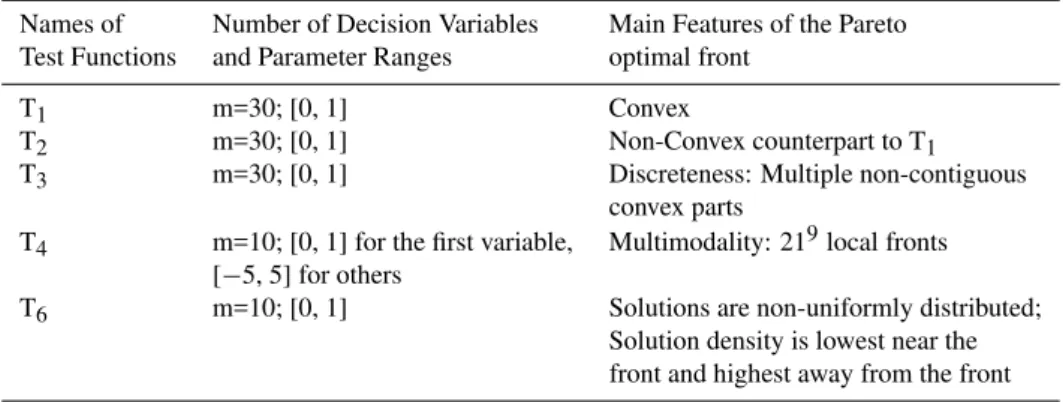
Table 1.Suite of test functions.
Names of Number of Decision Variables Main Features of the Pareto Test Functions and Parameter Ranges optimal front
T1 m=30; [0, 1] Convex
T2 m=30; [0, 1] Non-Convex counterpart to T1
T3 m=30; [0, 1] Discreteness: Multiple non-contiguous
convex parts
T4 m=10; [0, 1] for the first variable, Multimodality: 219local fronts
[−5, 5] for others
T6 m=10; [0, 1] Solutions are non-uniformly distributed; Solution density is lowest near the front and highest away from the front
adopts theε-dominance grid based approach for fitness as-signment and diversity preservation (Laumanns et al., 2002). Regarding the whole evolution process, MOSCEM-UA is significantly different from SPEA2 andε-NSGAII although all of them randomly initialize their search populations. As discussed above, MOSCEM-UA uses the complex shuffling method and the Metropolis-Hastings algorithm to conduct search. Offspring are generated using a multivariate normal distribution developed utilizing information from the current draw of the parallel sequence within a complex. The accep-tance of a new generated candidate solution is decided ac-cording to the scaled ratio of candidate solution’s fitness to current draw’s fitness of the sequence. Complex shuffling helps communication between different complexes and pro-motes solution diversity.
Comparatively, SPEA2 and ε-NSGAII adopt the tradi-tional evolutionary operators (e.g. selection, crossover and mutation) in searching. They both use binary tournament selection, simulated binary crossover (SBX), and polyno-mial mutation. And both of them maintain external archives which store the best solutions found from the random initial generation to final termination generation. However, these two algorithms are different in many aspects. After popu-lation initialization, SPEA2 assigns fitness to each individ-ual in the population and the archive. Nondominated sort-ing is conducted on all these individuals and then the non-dominated solutions are copied to the archive of next gener-ation. Because the archive is fixed in size, either a truncation scheme must be implemented or the best dominated solutions must be used to fill up the archive. Then binary tournament selection with replacement is applied to select individuals for a mating pool. The new population in SPEA2’s next genera-tion is created by applying crossover and mutagenera-tion operators to the mating pool. The process is repeated until a user spec-ified termination criterion is met.
ε-NSGAII initiates the search with an arbitrarily small number of individuals (e.g., 10-individuals). Binary tourna-ment selection, SBX crossover, and mutation operators are
implemented to generate the first child population. Pareto ranks are assigned to the individuals from the parent and chil-dren populations. Solutions are selected preferentially based on their non-domination rank. Crowding distances (i.e., Eu-clidean norms for measuring distance from neighbour solu-tions in objective space) are used to distinguish between the individuals with the same non-domination rank (i.e., larger crowding distances are picked preferentially to promote di-versity). At the end of each generation, the external archive is updated with theε-non-dominated solutions. The archive size and population size change dynamically based on the to-tal number ofεnon-dominated solutions stored. In this study, a single termination criterion based on the maximum num-ber of function evaluations was used for all of the algorithms (i.e., they all had identical numbers of function evaluations) to ensure a fair comparison.
3 Case studies
3.1 Case study 1: the test function suite
The first test case is composed of a standardized suite of com-puter science test problems (Zitzler et al., 2000; Deb, 2001; Coello Coello et al., 2002) that are used to validate the al-gorithms’ abilities to perform global search effectively, ef-ficiently, and reliably for a broad range of problem types. This is the first study to test MOSCEM-UA on this suite of problems. The test function suite has been developed col-laboratively by the EMO community (Coello Coello et al., 2002; Deb et al., 2002) as standardized performance tests where new algorithms must meet or exceed the performance of current benchmark algorithms such as SPEA2.
are labeled T1, T2, T3, T4, and T6 following the naming con-vention of Zitzler et al. (2000). All of the test functions have been implemented in the standard forms used in the EMO literature. Generally, T1 and T2 are considered relatively straightforward convex and non-convex test problems. T3 tests algorithms’ abilities to find discontinuous convex sets of solutions. T4 and T6 are the most challenging of the test functions requiring algorithms to overcome large numbers of local fronts and non-uniformly distributed solution spaces, respectively.
3.2 Case study 2: Leaf River watershed
The Leaf River SAC-SMA test case represents a benchmark problem within the water resources literature that has been used extensively for developing tools and strategies for im-proving hydrologic model calibration (Duan et al., 1992; Yapo et al., 1998; Boyle et al., 2000; Wagener et al., 2001; Vrugt et al., 2003a, b). Readers interested in the full de-tails of the Leaf River case study’s dataset should reference earlier works (e.g., Sorooshian et al., 1993). The Leaf River case study used in this paper has been developed based on the original studies used to develop and demonstrate MOSCEM-UA (Vrugt et al., 2003a, b). The Sacramento Soil Moisture Accounting model is a 16 parameter lumped conceptual wa-tershed model used for operational river forecasting by the National Weather Service throughout the US (see Burnash, 1995, for more details on the model). All three algorithms searched the same 13 SAC-SMA parameters (3 parameters are commonly fixed a priori) and parameter ranges as were specified by Vrugt et al. (2003a). The algorithms were tested on their ability to quantify a 2-objective tradeoff based on a root-mean square error (RMSE) problem formulation. The first objective was formulated using a Box-Cox transforma-tion of the hydrograph (z=[(y+1)λ−1]/λ whereλ=0.3) as recommended by Misirli et al. (2003) to reduce the impacts of heteroscedasticity in the RMSE calculations (also increas-ing the influence of low flow periods). The second objective was the non-transformed RMSE objective, which is largely dominated by peak flow prediction errors due to the use of squared residuals. The best known approximation set gener-ated for this problem is discussed in more detail in the results of this study (see Fig. 5a).
A 65-day warm-up period was used based on the method-ological recommendations of Vrugt et al. (2003a). A two-year calibration period was used from 1 October 1952 to 30 September 1954. The calibration period was shortened for this study to control the computational demands posed by rigorously assessing the EMO algorithms. A total of 150 EMO algorithm trial runs were used to characterize the al-gorithms (i.e., 50 trials per algorithm). Each EMO algo-rithm trial run utilized 100 000 SAC-SMA model evalua-tions, yielding a total of 15 000 000 SAC-SMA model evalu-ations used in our Leaf River case study analysis. Reducing the calibration period improved the computational
tractabil-ity of our analysis. The focus of this study is on assessing the performances of the three EMO algorithms that are captured in the 2 year calibration period. In actual operational use of the SAC-SMA for the Leaf River 8 to 10 year calibration pe-riods are used to account for climatic variation between years (Boyle et al., 2000).
3.3 Case study 3: Shale Hills watershed
The Shale Hills experimental watershed was established in 1961 and is located in the north of Huntington County, Penn-sylvania. It is located within the Valley and Ridge province of the Susquehanna River Basin in north central Pennsylva-nia. The data used in this study was supplied by a compre-hensive hydrologic experiment conducted in 1970 on a 19.8 acre sub-watershed of the Shale Hill experimental site. The experiment was led by Jim Lynch of the Pennsylvania State University’s Forestry group with the purpose of exploring the physical mechanisms of the formation of stream-flow at the upland forested catchment and to evaluate the impacts of an-tecedent soil moisture on both the volume and timing of the runoff (see Duffy, 1996). The experiment was composed of an extensive below canopy irrigation network for simu-lating rainfall events as well as a comprehensive piezometer network, 40 soil moisture neutron access tubes and 4 weirs for measuring flow in the ephemeral channel. Parameteriza-tion of the integrated surface-subsurface model for the Shale Hills was also supported by more recent site investigations, where Lin et al. (2005) extensively characterized the soil and groundwater properties of the site using in-situ observations and ground penetrating radar investigations.
1 3 2 4 5 6 7 I II III IV Outlet Outlet
1, 2, ..., 7 HRU 1, 2, ..., 7 HRU
I, II, III, IV River Sections I, II, III, IV River Sections
Fig. 1.Domain decomposition of the Shale Hills test case.
flexibility of easily adding/eliminating (switching on/off) the key hydrologic processes for a system.
As discussed above, the water budget is computed using a global model kernel composed of ODEs representing each of the watershed zones or river sections. The number of ODEs increases linearly with the number of decomposed spatial zones within the watershed. In the Shale Hills application, the watershed is decomposed into 7 zones and 4 river sections connected to each other between the zones. The decomposed domain and the topology of the zones and the river sections are shown in Fig. 1. The domain decomposition results in 32 ODEs solved implicitly using a solver that has been proven to be highly effective for ODE systems (Guglielmi and Hairer, 2001). The model simulation time is substantial for this study given that the EMO algorithms will have to evaluate thou-sands of simulations while automatically calibrating model parameters. On a Pentium 4 Linux workstation with a 3 gi-gahertz processor and 2 gigabytes of RAM, a one month sim-ulation of Shale Hills using a 1 h output time interval requires 120 s of computing time. If 5000 model evaluations are used to optimize model parameters, then a single EMO run will take almost 7 days. This study highlights how trial-and-error analysis of EMO algorithm performance can have a tremen-dous cost in both user and computational time.
3.3.2 Problem formulation
Multiobjective calibration uses multiple performance mea-sures to improve model predictions of distinctly different responses within a watershed’s hydrograph simultaneously (e.g., high flow, low flow, average flow). For the Shale Hills case study, the calibration objectives were formulated to generate alternative model parameter groups that cap-ture high flow, average flow, and low flow conditions for the Shale Hills test case using the three search objectives given in Eqs. (3)–(5). The problem formulations used in this study build on prior research using RMSE and the het-eroscedastic maximum likelihood estimator (HMLE) mea-sures (Sorooshian and Dracup, 1980; Yapo et al., 1996, 1998; Gupta et al., 1998; Boyle et al., 2000; Madsen, 2003; Ajami et al., 2004).
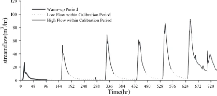
0 48 96 144 192 240 288 336 384 432 480 528 576 624 672 720 0 20 40 60 80 100 120 Time(hr) streamflow(m 3/hr)
Warm−up Perio d
Low Flow within Calibration Period High Flow within Calibration Period
Fig. 2. Illustration of the Shale Hills calibration period where a 100 h warm up period was used. High flow and low flow classifica-tions were made based on the points of inflection within the hydro-graph.
Average RMSE:f1(θ )=
"
1
N N
X
i=1
w1iQobs,i−Qsim,i(θ )2
#1/2
(3)
High flow RMSE:f2(θ )=
1 Mp P
j=1
nj Mp
X
j=1
nj
X
i=1
w2i
Qobs,i−Qsim,i(θ )
2
1/2
(4)
Low flow RMSE:f3(θ )=
1 Ml P
j=1
nj Ml
X
j=1
nj
X
i=1
w3i
Qobs,i−Qsim,i(θ )
2
1/2
(5)
whereQobs,iis the observed discharge at timei;Qsim,i(θ )
is the simulated discharge; N is the total number of time steps in the calibration period;Mpis the number of peak flow
events;Mlis the number of low flow events;nj is the
num-ber of time steps in peak/low flow event numnum-berj; w1,w2
andw3are the weighting coefficients;θis the set of model
parameters to be calibrated.
In this study, the weighting coefficients for high flow and low flow are adapted forms of the HMLE statistics (Yapo et al., 1996). The weights for high flow errors are set to the square of the observed discharges to emphasize peak dis-charge values. The weights for low flow are set to give prominence to low flow impacts on the estimation errors. The weighting coefficient for average flow is set to 1 and thus the error metric for average flow is the standard RMSE statis-tic. Equation (6) provides the weighting coefficients used to differentiate different hydrologic responses.
w1=1 w2=Q2obs w3=
1 Q2obs
!1/
Ml
P
j=1
nj
of the initial surface storage were attenuated within the first 100 h. Figure 2 illustrates the Shale Hills calibration period including a 100 h warm up period to reduce the impacts of the initial conditions. High flow and low flow classifications were made based on points of inflection within the hydro-graph. Table 2 overviews the parameters being calibrated for the Shale Hills case study. For overland flow, the conver-gence time scale of a hill slopeηcannot be estimated analyt-ically so the parameter was selected for calibration. The sat-urated soil hydraulic conductivityKsis calibrated as well as
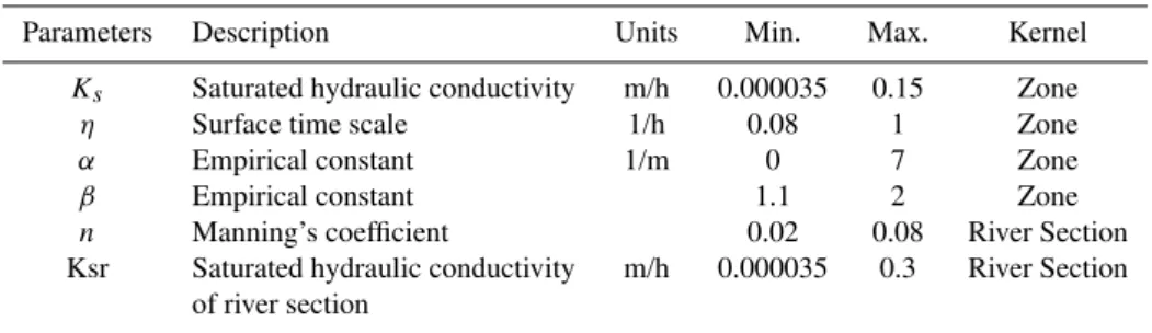
the empirical constants (α,β)in the van Genuchten soil func-tions. In our preliminary sensitivity analysis, Manning’s co-efficient (n)and the saturated hydraulic conductivity of river reaches were identified to significantly impact river routing and groundwater-stream interactions. Both of these parame-ters are calibrated. In the Shale Hills case study, a total of 36 parameters are being calibrated (7 spatial zones * 4 parame-ters + 4 river sections * 2 parameparame-ters). The parameter ranges were specified based on both field surveys (Qu, 2004; Lin et al., 2005) and recommendations from literature (Carsel, 1988; Dingman, 2002).
4 Description of the computational experiment
4.1 Algorithm configurations and parameterizations In an effort to ensure a fair comparison betweenε-NSGAII and each of the other algorithms, significant effort has been focused on seeking optimal configurations and parameteri-zations for SPEA2 and MOSCEM-UA using trial-and-error analysis and prior literature. The broadest analysis of the impacts of alternative algorithm configurations was done for the test function suite, since this test case has the small-est computational demands. The algorithms were allotted 15 000 function evaluations for each trial run when solv-ing each problem within the test function suite based on the recommendations and results of prior studies (Zitzler et al., 2001; Kollat and Reed, 2005a). For each problem in the test function suite a total of 350 trial runs were performed (i.e., 1 configuration forε-NSGAII tested for 50 random seeds, 4 MOSCEM-UA configurations tested for 50 random seeds each yielding 200 trial runs, and 2 SPEA2 configurations tested for 50 random seeds each yielding 100 trial runs).
Since ε-NSGAII and SPEA2 use the same mating and mutation operators, the algorithms’ probabilities of mating where set equal 1.0 and their probabilities of mutation were set equal to 1/L where L is the number of decision vari-ables as has been recommended extensively in the literature (Zitzler et al., 2000, 2001; Deb, 2001; Coello Coello et al., 2002). ε-NSGAII utilized an initial population size of 10 individuals. For the test function suite SPEA2’s two con-figurations both used an archive size of 100 based on prior studies (Zitzler et al., 2000, 2001; Deb, 2001; Coello Coello et al., 2002) and two different population sizes (N=100) and
(N=250). MOSCEM-UA’s configurations tested the impacts of increasing population sizesN and increasing the numbers of complexes C: (N=100, C=2), (N=250,C=2), (N=250, C=5) and (N=1000,C=5). The largest population size and number of complexes tested for MOSCEM-UA were based on a personal communication with Jasper Vrugt, the algo-rithm’s creator.
ε-NSGAII utilized the same configuration as was used for the test function suite on the Leaf River and Shale Hills case studies in an effort to test the algorithms’ robustness in the absence of trial-and-error analysis. Based on the SPEA2’s performance on the test function suite and trial-and-error analysis the algorithm’s population size was set equal to 100 for both the Leaf River and Shale Hills test cases. The key challenge in maximizing the performance of SPEA2 lies in specifying an effective archive size without a priori knowl-edge of the Pareto set. SPEA2’s performance is very sensi-tive to archive size. Trial-and-error analysis revealed that if the algorithm’s archive is too small then its overall perfor-mance suffered. Moreover, setting the SPEA2 archive to be very large also reduced the algorithm’s search effectiveness because its diversity enhancing clustering operator is under utilized. For the Leaf River and Shale Hills case studies, SPEA2’s performance was maximized by setting the archive size equal to 500 and 100, respectively, based on the aver-age archive sizes attained by theε-NSGAII. Noteε-NSGAII automatically sizes its archive based on the number of ε-nondominated solutions that have been found.
For the Leaf River case study, MOSCEM-UA utilized a population size of 500 individuals and 10 complexes as was used by Vrugt et al. (2003a) in the original development and demonstration of the algorithm. As will be discussed in the results presented in Sect. 5 increasing the population size and number of complexes used by MOSCEM-UA has a very large impact on the algorithm’s solution time, which signifi-cantly impacted our analysis of the Shale Hills test case. For the Shale Hills case study, MOSCEM-UA was tested for a population size of 250 with 2 or 5 complexes to ensure that a single run would complete in 7 days based on the maxi-mum run times allotted for the LION-XO computing clus-ter. The computational constraints limiting our ability to use larger population sizes and more complexes in the Shale Hills trial runs for MOSCEM-UA are discussed in greater detail in Sect. 5.
4.2 Performance metrics
opti-Table 2.Parameters being optimized in the Shale Hills case study.
Parameters Description Units Min. Max. Kernel
Ks Saturated hydraulic conductivity m/h 0.000035 0.15 Zone
η Surface time scale 1/h 0.08 1 Zone
α Empirical constant 1/m 0 7 Zone
β Empirical constant 1.1 2 Zone
n Manning’s coefficient 0.02 0.08 River Section Ksr Saturated hydraulic conductivity m/h 0.000035 0.3 River Section
of river section
mal solutions, and (2) diversity – how well the evolved set of solutions represents the full extent of the tradeoffs that ex-ist between an application’s objectives. Performance metrics that measure these properties are termed unary indicators be-cause their values are calculated using one solution set and they reveal specific aspects of solution quality (Zitzler et al., 2003).
Two unary metrics, theε-indicator (Zitzler et al., 2003) and the hypervolume indicator (Zitzler and Thiele, 1999) were selected to assess the performances of the algorithms. The unaryε-indicator measures how well the algorithms con-verge to the true Pareto set or the best known approximation to the Pareto set. The unaryε-indicator represents the small-est distance that an approximation set must be translated to dominate the reference set, so smaller indicator values are preferred. For example, in Fig. 3, the approximation set has to be translated a distance ofεso that it dominates the refer-ence set. The unary hypervolume metric measures how well the algorithms performed in identifying solutions along the full extent of the Pareto surface or its best known approxima-tion (i.e., soluapproxima-tion diversity). The unary hypervolume metric was computed as the difference between the volume of the objective space dominated by the true Pareto set and volume of the objective space dominated by the approximation set. For example, the blue shaded area in Fig. 3 represents the hypvervolume metric of the approximation set. Ideally, the hypervolume metric should be equal to zero. For more de-tails about the descriptions and usages of these metrics, see Zitzler and Thiele (1999); Zitzler et al. (2003); Kollat and Reed (2005b).
In addition to the unary metrics discussed above, perfor-mance was also assessed using the binary metric. The binary metric was implemented by combining the unaryε-indicator metric with an interpretation function. Zitzler et al. (2003) formulated the interpretation function to directly compare two approximation solution sets and conclude which set is better or if they are incomparable. The term “binary” refers to the metric’s emphasis on comparing the quality of two ap-proximation sets. Theε-indicator and the interpretation
func-Fig. 3. (a)Example illustration of theε-indicator metric. (b) Ex-ample illustration of the hypervolume metric. The shaded area with blue color represents the hypervolume value. Adapted from (Fon-seca et al., 2005).
tion are formulated as shown in Eqs. (7) and (8) separately: Iε(A, B)=max
f2∈Bminf1∈A1≤maxi≤n
fi1
fi2 (7)
F =(Iε(A, B)≤1∧Iε(B, A) >1) (8)
Where f1={f11, f21, ..., fn1}∈A and f2={f12, f22, ..., fn2}∈B are objective vectors;AandBare two approximation sets;F is an interpretation function. IfAis not better thanB andB is not better thanA, then the sets are incomparable. WhenF is true, it indicates thatAis better thanB. Similarly, chang-ing the order ofAandB, the decision about whetherB is better thanAcan be made.
0 1.5 3
0 2 4
0 1.5 3
0 60 120
0 3.75 7.5 11.25 15 0
4 8
0 3.75 7.5 11.25 15 0 3.75 7.5 11.25 15
-NSGAII SPEA2 MOSCEM-UA
Function Evaluations ( )
-Indicator
3
10
×
ε
ε
1 T
2 T
3 T
4 T
6 T
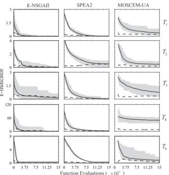
Fig. 4. Dynamic performance plot for the unaryε-indicator dis-tance metric versus total design evaluations for the best perform-ing configurations of theε-NSGAII, SPEA2, and MOSCEM. Mean performance is indicated by a solid line, the standard deviation by a dashed line, and the range of performance by the shaded region. The plots were generated using 50 trials for each algorithm.
are incomparable to one another. In this study, the binary ε-indicator ranking results are presented in terms of the ratio of trial runs that attain top ranks (i.e., ranks of 1 or 2).
5 Results
5.1 Optimization results for case study 1: test function suite
As described in Sect. 4.2, the binaryε-indicator metric pro-vides performance rankings for alternative algorithm con-figurations and cross-algorithm performance. For each test problem a total of 350 trial runs were performed (i.e., 1 configuration forε-NSGAII tested for 50 random seeds, 4 MOSCEM-UA configurations yielding 200 random seed tri-als, and 2 SPEA2 configurations yielding 100 random seed trials). After ranking the trial runs, we present the ratio of the number of top ranking runs out of the 50 trials used to test each of the algorithms’ configurations (see Table 3).
The best configurations for SPEA2 and MOSCEM-UA are (N=100) and (N=1000,C=5), respectively. Theε-NSGAII has the best overall binaryε-indicator metric rankings for the test function suite.
The unary hypervolume andε-indicator metrics measure solution diversity and algorithm convergence to the true
Pareto fronts, respectively. These unary metrics provide a more detailed understanding of the dynamic performances of the algorithms in terms of efficiency, effectiveness, and reliability. The means and standard deviations of the final optimization results for the best configurations (ε-NSGAII has only one configuration) are summarized in Table 4.
Recall that the unary ε-indicator represents the smallest distance that an approximation set must be translated to dom-inate the reference set so smaller indicator values are pre-ferred. Likewise, the unary hypervolume metric is the differ-ence between the volume of the objective space dominated by the true Pareto set and volume of the objective space dom-inated by the approximation set. Ideally, the hypervolume metric should be equal to zero.
In Table 4, theε-NSGAII has the best overall average per-formance in both metrics for the test functions. In addition, the relatively small standard deviations reveal thatε-NSGAII is reliable in solving the test functions. SPEA2 is also effec-tive and reliable in solving the test functions. Bothε-NSGAII and SPEA2 are superior to MOSCEM-UA. Figure 4 illus-trates the variability in the algorithms’ performances by pre-senting runtime results for theε-indicator distance metric.
The plots show the results of all 50 random seed trials with the mean performance indicated by a solid line, the stan-dard deviation by a dashed line, and the range of random seed performance indicated by the shaded region. Visualiz-ing the results in this manner allows for comparison between the dynamics and reliability (i.e., larger shaded regions indi-cate lower random seed reliability) of each algorithm.
com-Table 3.Test function results for the ratios of top trial runs for each configuration of the algorithms based on the binaryε-indicator metric ranking. The values highlighted by bold font are the best values among the configurations within a specific algorithm, the values indicated by bold font with underscore are the best values across algorithms.
MOEA Configurations Top Ranking Ratios
T1 T2 T3 T4 T6
ε-NSGAII (N=10) 50/50 50/50 50/50 50/50 50/50
SPEA2 (N=100) 50/50 9/50 50/50 1/50 47/50 (N=250) 50/50 6/50 45/50 0/50 27/50
MOSCEM-UA
(N=100,C=2) 0/50 0/50 0/50 0/50 6/50 (N=250,C=2) 1/50 0/50 0/50 0/50 12/50 (N=250,C=5) 0/50 0/50 0/50 0/50 14/50 (N=1000,C=5) 11/50 0/50 0/50 0/50 20/50
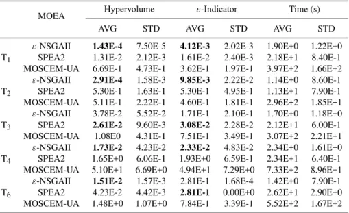
Table 4.Averages and standard deviations of the unary metrics for each algorithm’s best configuration. AVG stands for mean, STD stands for standard deviation, and bolded entries highlight the best value attained.
MOEA Hypervolume ε-Indicator Time (s)
AVG STD AVG STD AVG STD
ε-NSGAII 1.43E-4 7.50E-5 4.12E-3 2.02E-3 1.90E+0 1.22E+0 T1 SPEA2 1.31E-2 2.12E-3 1.61E-2 2.40E-3 2.18E+1 8.40E-1
MOSCEM-UA 6.69E-1 4.73E-1 3.62E-1 1.97E-1 3.97E+2 1.66E+2
ε-NSGAII 2.91E-4 1.58E-3 9.85E-3 2.22E-2 1.14E+0 8.60E-1 T2 SPEA2 5.30E-1 1.63E-1 5.30E-1 4.95E-1 1.13E+1 7.90E-1
MOSCEM-UA 5.11E-1 2.22E-1 4.60E-1 1.81E-1 2.96E+2 1.85E+1
ε-NSGAII 3.78E-2 5.52E-2 1.71E-1 2.10E-1 1.70E+0 1.18E+0 T3 SPEA2 2.61E-2 9.60E-3 3.08E-2 2.28E-2 2.12E+1 6.00E-1 MOSCEM-UA 1.08E0 4.31E-1 7.51E-1 3.49E-1 3.07E+2 2.21E+1
ε-NSGAII 1.73E-2 4.23E-2 2.33E-2 4.83E-2 2.34E+0 1.61E+0 T4 SPEA2 1.65E+0 6.06E-1 1.93E+0 6.59E-1 2.34E+1 6.40E-1
MOSCEM-UA 5.10E+1 6.69E+0 4.94E+1 7.29E+0 7.33E+2 8.96E+1
ε-NSGAII 1.51E-2 1.57E-3 2.81E-1 1.68E-4 1.42E+0 7.90E-1 T6 SPEA2 4.23E-2 4.42E-3 2.81E-1 0.00E+0 2.62E+1 2.90E+0
MOSCEM-UA 1.48E+0 1.07E+0 7.84E-1 3.39E-1 5.52E+2 1.67E+2
putational times required for our test function analysis, where several days were required for MOSCEM-UA, several hours for SPEA2, and several minutes forε-NSGAII.
Averaged performance metrics are meaningful only in cases when the EMO algorithms’ metric distributions are sig-nificantly different from one another. In this study, the Mann-Whitney test (Conover, 1999) was used to validate that the algorithms attained statistically significant performance dif-ferences. The null hypothesis for the tests assumed that met-ric distributions for any two algorithms are the same. The Mann-Whitney test showed a greater than 99% confidence that performance metric scores for theε-NSGAII are sig-nificantly different from those of MOSCEM-UA for all of the test functions. When comparing SPEA2 and MOSCEM-UA it was found that the algorithms’ performance differences
on T2 are not statistically significant. On all of the remain-ing test functions SPEA2’s superior performance relative to MOSCEM-UA was validated at greater than a 99% confi-dence level. Theε-NSGAII’s performance was statistically superior to SPEA2 at the 99% confidence level for all of the test functions except for T3. ε-NSGAII and SPEA2 did not attain a statistically meaningful performance difference on T3.
5.2 Optimization results for case study 2: leaf river water-shed
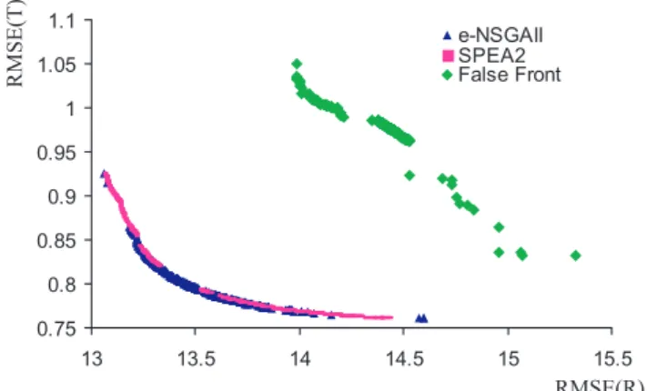
gener-0.75 0.8 0.85 0.9 0.95 1 1.05 1.1
13 13.5 14 14.5 15 15.5
e-NSGAII SPEA2 False Front
RMSE(R)
RMSE(T)
Fig. 5. (a)Reference set generated for the Leaf River test case where RMSE(T) are the errors for the Box-Cox transform of the hydrograph and RMSE(R) are the errors for the raw hydrograph. The figure also shows a false front that often trapped the algorithms. (b)The percentage of the reference set contributed byε-NSGAII, SPEA2, and MOSCEM-UA.
Table 5.Leaf River case study’s ratios of top trial runs for each con-figuration of the algorithms based on the binaryε-indicator metric ranking. The best performing algorithm is highlighted in bold.
MOEA Configurations Top Ranking Ratios
ε-NSGAII (N=10) 23/50
SPEA2 (N=100) 42/50
MOSCEM-UA (N=500,C=10) 13/50
ated by collecting all of the nondominated solutions gener-ated from the 150 trial runs used for this case study (i.e., 50 trial runs per algorithm). Figure 5 shows the solutions con-tributed by each algorithm for the 2-objective tradeoff be-tween the Box-Cox transformed RMSE metric and the stan-dard RMSE metric.
ε-NSGAII found 58% of the reference set and the re-maining 42% of the reference set was generated by SPEA2. MOSCEM-UA was unable to contribute to the best solutions that compose the reference set. Table 5 shows that SPEA2 was able to attain the best binaryε-indicator metric rankings followed byε-NSGAII and lastly MOSCEM-UA.
Table 6 shows that SPEA2 had the best average per-formance in terms of both the ε-indicator and hypervol-ume unary metrics. The Mann-Whitney test validated that SPEA2’s results were different from both MOSCEM-UA and ε-NSGAII at the 99% confidence level.
The results of Table 6 demonstrate that average perfor-mance metrics can be misleading without statistical testing. Although MOSCEM-UA has superior mean hypervolume andε-indicator distance values relative to ε-NSGAII, per-formance differences between the algorithms were not sta-tistically significant (i.e., the null hypothesis in the
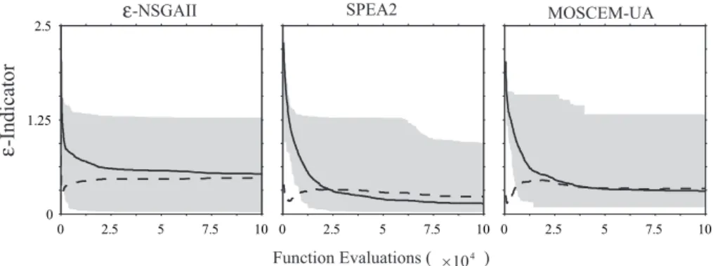
Mann-Whitney test could not be rejected). In fact, all three algo-rithms had significant ranges of performance for this test case because of the presence of a large false front (i.e., the locally nondominated front shown in Fig. 5) that caused some of the algorithms’ runs to miss the best known front. Figure 6 illustrates the variability in the algorithms’ performances by presenting runtime results for theε-indicator distance metric. Figure 6 verifies that SPEA2 has the best mean perfor-mance over the full duration of the run. The figure also shows that SPEA2 was slightly more reliable relative toε-NSGAII and MOSCEM-UA. Dynamic plots for hypervolume showed similar runtime distributions for the three algorithms. Fig-ure 7 illustrates dynamic results for the best trial runs for each of the algorithms. The best trial runs were selected based on the algorithms’ best unary metrics scores.
The plot shows thatε-NSGAII is able to attain superior hy-pervolume (diversity) andε-indicator distance (convergence) metrics in less than 5000 model evaluations. SPEA2 and MOSCEM-UA required between 12 000 and 25 000 model evaluations to attain equivalent performance metric values. Overall SPEA2 had superior performance for this test case while MOSCEM-UA andε-NSGAII had comparable perfor-mances.
5.3 Optimization results for case study 3: Shale Hills wa-tershed
0 2.5 5 7.5 10 0
1.25 2.5
0 2.5 5 7.5 10 0 2.5 5 7.5 10
Function Evaluations ( )
-Indicator
ε
-NSGAII SPEA2 MOSCEM-UA
ε
4
10 ×
Fig. 6. Leaf River test case dynamic performance results for the unaryε-indicator distance metric versus total design evaluations. Mean performance is indicated by a solid line, the standard deviation by a dashed line, and the range of performance by the shaded region. The plots were generated using 50 trial runs for each algorithm.
Table 6.Leaf River case study’s results for the averages and standard deviations of the unary metrics for each algorithm configuration. AVG stands for mean, STD stands for standard deviation, and bolded entries highlight the best value attained.
MOEA Hypervolume ε-Indicator Time (s)
AVG STD AVG STD AVG STD
ε-NSGAII 1.11E+0 1.04E+0 5.31E-1 4.78E-1 8.29E+2 3.58E+1 SPEA2 2.96E-1 4.32E-1 1.39E-1 2.30E-1 8.33E+2 1.82E+1 MOSCEM-UA 5.49E-1 6.49E-1 3.05E-1 3.34E-1 1.24E+3 5.95E+1
Table 7.Shale Hills case study’s ratios of top trial runs for each con-figuration of the algorithms based on the binaryε-indicator metric ranking. The best performing algorithm is highlighted in bold.
MOEA Configurations Top Ranking Ratios
ε-NSGAII (N=10) 14/15
SPEA2 (N=100) 15/15
MOSCEM-UA (N=250,C=2) 4/15 (N=250,C=5) 6/15
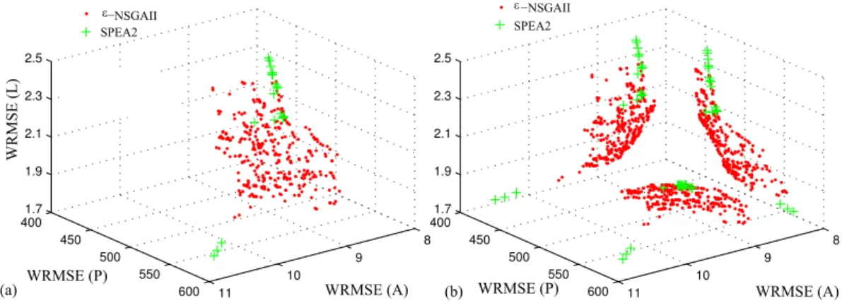
The best known approximation set was generated by col-lecting the nondominated solutions from the 60 trial runs used for this case study. Figure 8a shows the best known solution set in the 3-objective solution space defined for this test case. Figure 8b projects the solution set onto the 2-objective planes to better illustrate the tradeoffs that exist be-tween low, average, and peak flow calibration errors.
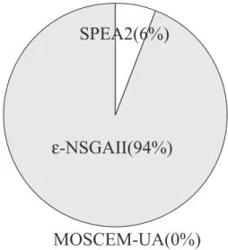
Figure 9 shows thatε-NSGAII found 94% of the reference set and the remaining 6% of the reference set was generated by SPEA2. MOSCEM did not contribute to the best solutions that compose the reference set.
Table 7 shows that SPEA2 was able to attain slightly better binaryε-indicator metric rankings relative to theε-NSGAII. As indicated by Fig. 9 and Table 7 MOSCEM had
diffi-Table 8. Shale Hills case study’s results for the averages and stan-dard deviations of the unary metrics for each algorithm configura-tion. AVG stands for mean, STD stands for standard deviation, and bolded entries highlight the best value attained.
MOEA Hypervolume ε-Indicator
AVG STD AVG STD
ε-NSGAII 2.09E+04 1.82E+04 1.18E+0 1.95E-1 SPEA2 1.63E+04 7.17E+03 1.12E+0 4.46E-2 MOSCEM-UA 4.71E+04 1.93E+04 1.38E+0 2.22E-1
cultly in generating highly ranked runs for this test case. Al-though Table 8 shows that SPEA2 had the best average per-formance in terms of theε-indicator and hypervolume unary metrics, the Mann-Whitney test showed that SPEA2’s results were not statistically different fromε-NSGAII. Relative to MOSCEM-UA, SPEA2 andε-NSGAII attained superior re-sults that were confirmed to be statistically different at the 99% confidence level.
Function Evaluations ( )
Hypervolume
-Indicator
ε
4
10
×
0 2.5 5 7.5 10
0 2.5 5
ε−NSGAII SPEA2 MOSCEM−UA
0 2.5 5 7.5 10
0 1.25
2.5
ε−NSGAII SPEA2 MOSCEM−UA
Fig. 7.Dynamic performance plots showing the best performing Leaf River trial runs for each algorithm.
WRMSE (P)
WRMSE (P)
WRMSE (A) WRMSE (A)
WRMSE (L)
(a) (b)
8 9 10 11 400
450 500
550 600 1.7
1.9 2.1 2.3 2.5
8 9 10 11 400
450 500
550 600 1.7
1.9 2.1 2.3 2.5
ε−NSGAII SPEA2
ε −NSGAII SPEA2
Fig. 8. (a)Reference set for the Shale Hills test case(b)projections of the reference set onto the 2-objective planes to highlight the tradeoffs between the objectives.
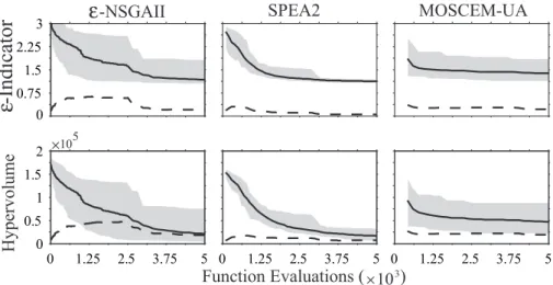
based on the algorithms’ best unary metrics scores. Per-formance metric differences between SPEA2 andε-NSGAII resulted from a single trial run. As shown in Table 7 a singleε-NSGAII run failed to attain a top binary ranking, which is reflected in the upper bound of the shaded region in Fig. 10. This single run highly biased both the mean and standard deviations for the unary metrics given in Table 8 for ε-NSGAII. The Mann-Whitney test validates that the remain-ingε-NSGAII trial runs were not statistically different from SPEA2. For MOSCEM-UA, Table 7 in combination with Fig. 10 show that more than 60 percent of the algorithm’s trial runs failed to solve this test case. Figures 9 and 11 show thatε-NSGAII’s best runs were superior relative to the other algorithms’ results, generating nearly all of the reference set. As was noted for the Leaf River case study, SPEA2’s per-formance for the Shale Hills test case is heavily impacted by its archive size. It has been widely recognized (Coello Coello et al., 2002) that SPEA2’sk-means clustering diversity op-erator allows the algorithm to attain highly diverse solution sets for high-order Pareto optimization problems (i.e., prob-lems with 3 or more objectives). This operator is only
ac-tive in the search process if the archive is sized appropriately, which in typical applications will require trial-and-error anal-ysis. For this test case every trial run would require a week of computing time. It should be noted thatε-NSGAII auto-matically generates its archive size based on users’ precision goals for each objective. Additionally, the algorithm starts with a very small population size, which is automatically ad-justed to enhance search effectiveness. The results presented in this study are conservative tests for theε-NSGAII because SPEA2 and MOSCEM-UA initiate search with at least an or-der of magnitude advantage in search population.
6 Discussion
6.1 Relative benefits and limitations of SPEA2
difficult multimodal problem with 219local fronts. SPEA2’s best overall performance occurred for the Leaf River case study where the algorithm was far more reliable relative to both theε-NSGAII and MOSCEM-UA. The Leaf River test case is challenging because of its multimodality (see Fig. 5). Our analysis showed that carefully setting the archive size for SPEA2 for this case study enabled the algorithm to fully exploit its k-means clustering diversity operator to spread so-lutions across the search space and more reliably escape the false nondominated front shown in Fig. 5. For the Shale Hills test case, SPEA2 andε-NSGAII had statistically equivalent performance metrics, although SPEA2 was slightly more re-liable. SPEA2 is generally superior in performance relative to MOSCEM-UA.
The primary strengths of the SPEA2 algorithm lie in the al-gorithm’s search reliability and its diversity preservation op-erator as has been recognized in other studies. In this study, SPEA2 showed a limited sensitivity to its population sizing and search parameters. Other studies (Zitzler et al., 2001; Coello Coello et al., 2002; Deb et al., 2003) have shown that SPEA2’s sensitivity to population size often manifests itself in terms of a performance threshold for very difficult prob-lems where the algorithm fails until the population is made sufficiently large. In this study, SPEA2’s poor performance on test function T4 provides an example of this performance threshold. In these cases, it is very difficult to predict how to appropriately size SPEA2’s population. Significant trial-and-error analysis is required. The biggest challenge in maximiz-ing the performance of SPEA2 lies in specifymaximiz-ing an effective archive size without a priori knowledge of the Pareto set. In practice, this would require significant trial-and-error analy-sis, which is problematic for more complex, computationally intensive calibration applications.
6.2 Relative benefits and limitations of MOSCEM-UA MOSCEM-UA was the least competitive of the three algo-rithms tested in this study failing to effectively solve ei-ther the standardized test function suite or the Shale Hills test case. MOSCEM-UA attained its best performance on the Leaf River case study, which was used in its develop-ment (Vrugt et al., 2003a). On the Leaf River case study, MOSCEM-UA was inferior to SPEA2 and statistically simi-lar toε-NSGAII. MOSCEM-UA did not contribute to any of the reference sets (i.e., the best overall solutions) for the two hydrologic calibration applications. The algorithm’s Markov Chain Monte Carlo sampler in combination with its shuffle complex search operator does not scale well for problems of increasing size and/or difficulty. MOSCEM-UA’s binary ε-indicator rankings for all three test cases show that the al-gorithm is not reliable even with significant increases in pop-ulation size and the number of complexes.
MOSCEM-UA’s primary strength is its estimation of the posterior parameter distributions for hydrologic model pa-rameters (assuming the initial Gaussian assumptions made
MOSCEM-UA(0%)
-NSGAII(94%)
SPEA2(6%)
ε
Fig. 9.The percentages of the Shale Hills reference set contributed byε-NSGAII, SPEA2, and MOSCEM-UA.
for hydrologic parameters are acceptable to users). Addi-tionally, the algorithm has a limited number of parameters that need to be specified (i.e., the population size, run length, and number of complexes). MOSCEM-UA is however, crit-ically sensitive to these parameters. The matrix inversion used in the algorithm’s stochastic search operators causes MOSCEM-UA’s efficiency to dramatically reduce with in-creases in population size and inin-creases in the number of complexes. The algorithm is best suited for hydrologic model calibration applications that have small parameter sets and small model evaluation times. In general, it would be expected that MOSCEM-UA’s performance would be met or exceeded by either SPEA2 orε-NSGAII.
6.3 Relative benefits and limitations ofε-NSGAII
ε-NSGAII attained competitive to superior performance re-sults relative to SPEA2 on the test function suite and the Shale Hills test case. Overall,ε-NSGAII generated the ma-jority the reference sets (i.e., best overall solutions) for both hydrologic model calibration case studies. ε-NSGAII also had the best single run results for both of the calibration case studies as illustrated in Figs. 7 and 11. The algorithm’s poor-est performance occurred on Leaf River case study, in which its average performance was inferior to SPEA2 and statisti-cally equivalent to MOSCEM-UA.
0 0.75 1.5 2.25 3
0 1.25 2.5 3.75 5
0 0.5 1 1.5 2
0 1.25 2.5 3.75 5 0 1.25 2.5 3.75 5
Function Evaluations ( )
-NSGAII
SPEA2
MOSCEM-UA
-Indicator
3
10
×
ε
ε
Hypervolume
5 10
×
Fig. 10.Shale Hills test case dynamic performance results for the unaryε-indicator distance metric versus total design evaluations. Mean performance is indicated by a solid line, the standard deviation by a dashed line, and the range of performance by the shaded region. The plots were generated using 15 trial runs for each algorithm.
Function Evaluations ( )
310
×
-Indicator
ε
Hypervolume
5 10 ×
0 1.25 2.5 3.75 5
0 0.5 1 1.5 2
ε−NSGAII
SPEA2 MOSCEM−UA
0 1.25 2.5 3.75 5
1 1.5 2 2.5 3
ε−NSGAII
SPEA2 MOSCEM−UA
Fig. 11.Dynamic performance plots showing the best performing Shale Hills trial runs for each algorithm.
its crowded tournament diversity operator can fail to promote sufficient diversity for some problems. Although Kollat and Reed (2005a, b) have demonstratedε-NSGAII is statistically superior to the original NSGAII in terms of both convergence and diversity,ε-NSGAII can still be impacted by the limita-tions associated with the crowded tournament operator. For the Leaf River case study,ε-NSGAII had a reduced reliability relative to SPEA2 because several trial runs failed to create sufficiently diverse solutions that could escape the false local front. As was discussed above, SPEA2’s archive was sized carefully to maximize the effectiveness of its k-means clus-tering diversity operator, which allowed the algorithm to es-cape the local front. It is interesting to note that for the multi-modal T4 test function with 219local fronts, thatε-NSGAII’s performance is far superior to SPEA2. In this instance, ε-NSGAII’s was able to escape local fronts because of the ran-dom solutions injected into the search population during the
algorithm’s dynamic changes in population size. In the limit, when the algorithm’sε-dominance archive size stabilizes, the ε-NSGAII’s dynamic population sizing and random solution injection is equivalent to a diversity enhancing search opera-tor termed “time continuation” (Goldberg, 2002).
7 Conclusions
This study provides a comprehensive assessment of state-of-the-art evolutionary multiobjective optimization tools’ rela-tive effecrela-tiveness in calibrating hydrologic models. Three test cases were used to compare the algorithms’ perfor-mances. The first test case is composed of a standardized suite of computer science test problems, which are used to validate the algorithms’ abilities to perform global search ef-fectively, efficiently, and reliably for a broad range of prob-lem types. The ε-NSGAII attained the best overall per-formance for the test function suite followed by SPEA2. MOSCEM-UA was not able to solve the test function suite reliably. The second test case is a benchmark hydrologic calibration problem in which the Sacramento soil moisture accounting model is calibrated for the Leaf River water-shed. SPEA2 attained statistically superior performance for this case study in all metrics at the 99% confidence level. MOSCEM-UA and ε-NSGAII attained results that were competitive with one another for the Leaf River case study. The third test case assesses the algorithms’ performances for a computationally intensive integrated hydrologic model cal-ibration application for the Shale Hills watershed located in the Susquehanna River Basin in north central Pennsylvania. For the Shale Hills test case, SPEA2 andε-NSGAII had sta-tistically equivalent performance metrics, although SPEA2 was slightly more reliable. MOSCEM-UA’s performance on the Shale Hills test case was limited by the severe computa-tional costs associated with increasing the algorithm’s popu-lation size and number of complexes.
Overall, SPEA2 is an excellent benchmark algorithm for multiobjective hydrologic model calibration. SPEA2 at-tained competitive to superior results for most of the prob-lems tested in this study. The primary strengths of the SPEA2 algorithm lie in its search reliability and its diversity preser-vation operator. The biggest challenge in maximizing the performance of SPEA2 lies in specifying an effective archive size without a priori knowledge of the Pareto set. In prac-tice, this would require significant trial-and-error analysis, which is problematic for more complex, computationally in-tensive calibration applications.ε-NSGAII appears to be su-perior to MOSCEM-UA and competitive with SPEA2 for hydrologic model calibration. ε-NSGAII’s primary strength lies in its ease-of-use due to its dynamic population sizing and archiving which lead to rapid convergence to very high quality solutions with minimal user input. MOSCEM-UA is best suited for hydrologic model calibration applications that have small parameter sets and small model evaluation times. In general, it would be expected that MOSCEM-UA’s performance would be met or exceeded by either SPEA2 or ε-NSGAII. Future hydrologic calibration studies are needed to test emerging algorithmic innovations combining global multiobjective methods and local search (e.g., see Solo-matine, 1998; SoloSolo-matine, 1999; Ishibuchi and Narukawa, 2004; Krasnogor and Smith, 2005; Solomatine, 2005).
Acknowledgements. This work was partially supported by the National Science Foundation under grants EAR-0310122 and EAR-0418798. Any opinions, findings and conclusions or rec-ommendations expressed in this paper are those of the writers and do not necessarily reflect the views of the National Science Foundation. Additional support was provided by the Pennsylvania Water Resources Center under grant USDI-01HQGR0099. Partial support for the third author was provided by SAHRA under NSF-STC grant EAR-9876800, and the National Weather Service Office of Hydrology under grant numbers NOAA/NA04NWS4620012, UCAR/NOAA/COMET/S0344674, NOAA/DG 133W-03-SE-0916.
Edited by: D. Solomatine
References
Ajami, N. K., Gupta, H. V., Wagener, T., and Sorooshian, S.: Cal-ibration of a semi-distributed hydrologic model for streamflow estimation along a river system, J. Hydrol., 298, 112–135, 2004. Boyle, D. P., Gupta, H. V., and Sorooshian, S.: Toward improved calibration of hydrologic models: Combining the strengths of manual and automatic methods, Water Resour. Res., 36, 3663– 3674, 2000.
Burnash, R. J. C.: The NWS river forecast system-Catchment model, in: Computer Models of Watershed Hydrology, edited by: Singh, V. P., Water Resources Publications, Highlands Ranch, CO, 1995.
Carsel, R. F.: Developing joint probability distributions of soil water retention characteristics, Water Resour. Res., 24, 755–769, 1988. Cieniawski, S. E., Eheart, J. W., and Ranjithan, S. R.: Using ge-netic algorithms to solve a multiobjective groundwater monitor-ing problem, Water Resour. Res., 31, 399–409, 1995.
Coello Coello, C., Van Veldhuizen, D. A., and Lamont, G. B.: Evolutionary Algorithms for Solving Multi-Objective Problems, Kluwer Academic Publishers, New York, 2002.
Conover, W. J.: Practical Nonparametric Statistics , 3rd edition, John Wiley & Sons, New York, 1999.
Deb, K.: Multi-Objective Optimization using Evolutionary Algo-rithms, John Wiley & Sons LTD., New York, 2001.
Deb, K. and Jain, S.: Running Performance Metrics for Evolution-ary Multi-Objective Optimization, 2002004, Indian Institute of Technology Kanpur, Kanpur, India, 2002.
Deb, K., Mohan, M., and Mishra, S.: A Fast Multi-objective Evolu-tionary Algorithm for Finding Well-Spread Pareto-Optimal So-lutions, KanGAL Report No. 2003002, Indian Institute of Tech-nology, Kanpur, India, 2003.
Deb, K., Pratap, A., Agarwal, S., and Meyarivan, T.: A Fast and Elitist Multiobjective Genetic Algorithm: NSGA-II, IEEE Trans. Evol. Computation, 6, 182-197, 2002.
Deb, K., Thiele, L., Laumanns, M., and Zitzler, E.: Scalable multi-objective optimization test problems, in: In Proceedings of the Congress on Evolutionary Computation (CEC-2002), pp. 825– 830, 2002.
Dingman, S. L.: Physical Hydrology, Second Edition edition, Pren-tice Hall, New Jersey, 2002.