www.geosci-model-dev.net/8/4045/2015/ doi:10.5194/gmd-8-4045-2015
© Author(s) 2015. CC Attribution 3.0 License.
Coupling global models for hydrology and nutrient loading to
simulate nitrogen and phosphorus retention in surface water –
description of IMAGE–GNM and analysis of performance
A. H. W. Beusen1,2, L. P. H. Van Beek3, A. F. Bouwman1,2, J. M. Mogollón1, and J. J. Middelburg1
1Department of Earth Sciences – Geochemistry, Faculty of Geosciences, Utrecht University, PO Box 80021,
3508 TA Utrecht, the Netherlands
2PBL Netherlands Environmental Assessment Agency, P.O. Box 303, 3720 AH Bilthoven, the Netherlands 3Department of Physical Geography, Faculty of Geosciences, Utrecht University, P.O. Box 80.115,
3508 TC Utrecht, the Netherlands
Correspondence to:A. H. W. Beusen ([email protected])
Received: 1 June 2015 – Published in Geosci. Model Dev. Discuss.: 3 September 2015 Revised: 18 November 2015 – Accepted: 1 December 2015 – Published: 21 December 2015
Abstract. The Integrated Model to Assess the Global Environment–Global Nutrient Model (IMAGE–GNM) is a global distributed, spatially explicit model using hydrology as the basis for describing nitrogen (N) and phosphorus (P) delivery to surface water, transport and in-stream retention in rivers, lakes, wetlands and reservoirs. It is part of the in-tegrated assessment model IMAGE, which studies the inter-action between society and the environment over prolonged time periods. In the IMAGE–GNM model, grid cells receive water with dissolved and suspended N and P from upstream grid cells; inside grid cells, N and P are delivered to water bodies via diffuse sources (surface runoff, shallow and deep groundwater, riparian zones; litterfall in floodplains; atmo-spheric deposition) and point sources (wastewater); N and P retention in a water body is calculated on the basis of the residence time of the water and nutrient uptake velocity; sub-sequently, water and nutrients are transported to downstream grid cells. Differences between model results and observed concentrations for a range of global rivers are acceptable given the global scale of the uncalibrated model. Sensitivity analysis with data for the year 2000 showed that runoff is a major factor for N and P delivery, retention and river export. For both N and P, uptake velocity and all factors used to com-pute the subgrid stream retention are important for total in-stream retention and river export. Soil N budgets, wastewater and all factors determining litterfall in floodplains are impor-tant for N delivery to surface water. For P the factors that
determine the P content of the soil (soil P content and bulk density) are important factors for delivery and river export.
1 Introduction
Eutrophication, induced by a surge in anthropogenic nutri-ent loads to the global freshwater domain (e.g., rivers, lakes and estuaries), has an increasingly negative impact on aquatic ecosystems. In order to ameliorate and reverse this trend, ecological principles must be integrated into environmental management and restoration practices. These actions require a thorough understanding of the interactions between various human-induced disturbances (e.g., climate change, land use change, nutrient loadings and hydrology regulation) and their effects on freshwater systems (Stanley et al., 2010). To fully grasp the human impact on biogeochemical cycles, studies must collectively consider the biogeochemical turnover and exchange among the atmosphere, and the aquatic and terres-trial ecosystems.
at least two key reasons for this: (i) many of these issues are strongly interlinked and integrated models can capture im-portant consequences of these linkages; and (ii) substantial inertia is an inherent property of these problems, which can only be captured using long-term scenarios.
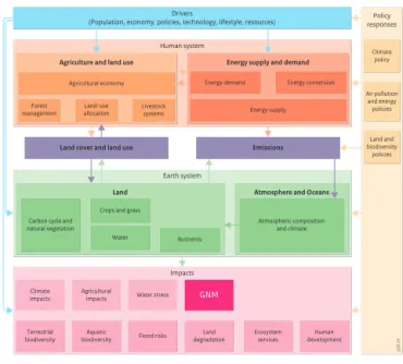
The Integrated Model to Assess the Global Environment (IMAGE) (Stehfest et al., 2014) is an IAM. IMAGE is struc-tured around key global sustainability problems (Fig. 1). Similar to other IAMs, it contains two main subcomponents: i.e., (i) the human system, describing the long-term devel-opment of human activities relevant for sustainable develop-ment issues, and (ii) the Earth system, describing changes in the natural environment. The two systems are coupled via the impact of human activities on the environment, and via the impacts of environmental change back on the human system. This paper describes the IMAGE–Global Nutrient Model (GNM), which simulates the fate of nitrogen (N) and phosphorus (P) in surface water arising from concentrated point sources (wastewater from urban and rural popula-tions, and industrial wastewater), and from dispersed (non-point) sources such as agricultural production systems with its fertilizer application and manure management, and nat-ural ecosystems. This global-scale model focuses on pro-longed historical periods for testing output results, and fu-ture scenarios to analyze consequences of fufu-ture global change. IMAGE–GNM uses the grid-based global hydrologi-cal model PCRaster Global Water Balance (PCR-GLOBWB) (Van Beek et al., 2011) to quantify water stores and fluxes, volume, surface area, and thus depth of water bodies, and water travel time. IMAGE–GNM takes spatially explicit in-put from the IMAGE land model, including land cover and the annual surface N balance from inputs such as biological N fixation, atmospheric N deposition and the usage of syn-thetic N fertilizer and animal manure. The IMAGE–GNM model comprises processes such as N removal due to crop harvesting, hay and grass cutting and grazing (Fig. 1). Start-ing from the soil nutrient budgets, IMAGE–GNM simulates the outflow of nutrients from the soil in combination with emissions from point sources and direct atmospheric depo-sition to determine the nutrient load to surface water and its fate during transport via surface runoff. It furthermore tracks nutrient transport in groundwater, riparian zones, lakes and reservoirs and in-stream biogeochemical retention processes. Earlier versions of parts of this model, particularly for the nu-trient flows towards surface water, have been described previ-ously for N (Van Drecht et al., 2003; Bouwman et al., 2013a), where the retention of N in streams, rivers, lakes and reser-voirs was represented by a single, global coefficient. A first step to improve these approaches was the coupling of IM-AGE with a hydrological model at the global scale to analyze N retention as pioneered by Wollheim et al. (2008a). Follow-ing Wollheim et al. (2008a), the version of IMAGE–GNM presented here uses the nutrient spiraling approach (Newbold et al., 1981) to describe in-stream retention of both total N and total P with a yearly time step.
IMAGE 3.0 framework
Source: PBL 2014
Drivers
(Population, economy, policies, technology, lifestyle, resources)
Climate policy
Air pollution and energy policies
Land and biodiversity
policies
Policy responses
Human system
Earth system
Impacts
Agricultural economy
Land cover and land use Emissions Energy supply and demand
Land-use allocation Forest
management
Livestock systems
Agriculture and land use
Land Atmosphere and Oceans
Energy demand Energy conversion
Atmospheric composition and climate Carbon cycle and
natural vegetation
Crops and grass
Water Nutrients
Energy supply
Climate impacts
Agricultural
impacts Water stress GNM
Terrestrial biodiversity
Aquatic
biodiversity Flood risks Land degradation
Ecosystem services
Human development
pbl.nl
Figure 1.Scheme of the Integrated Model to Assess the Global Environment (IMAGE) modified from Stehfest et al. (2014).
In summary, IMAGE–GNM is a global, spatially explicit model, which uses hydrology as the basis for describing N and P delivery to surface water and in-stream transport and retention. It is part of the IAM IMAGE, and used to study the impact of multiple environmental changes over time frames, which capture the mutual feedbacks between humanity and the Earth system. In this manuscript, we compare the model behavior against observations for a number of rivers, and test its sensitivity to a range of model parameter variations to an-alyze the impact of changing nutrient loading, climate and hydrology.
2 Model description 2.1 General aspects
The IMAGE model utilizes historical data for testing the model behavior, and projections to describe direct and in-direct drivers of future global environmental change. Most of these drivers (such as technology and lifestyle assump-tions) are used as input in various subcomponents of IMAGE such as GNM (Fig. 1). Clearly, the exogenous assumptions made on these factors need to be consistent. To ensure this, so-called storylines are used, brief descriptions about how the future may unfold, that can be used to derive internally consistent assumptions for the main driving forces of each IMAGE module. Important categories of scenario drivers in-clude demographic factors, economic development, lifestyle and technology change. Among these, population and eco-nomic development form a special category as they can be dealt with in a quantitative sense as exogenous model drivers. The geographical resolution of IMAGE 3.0 is 26 socio-economic world regions (Stehfest et al., 2014). These regions are selected given their relevance for global environmental problems and a relatively high degree of internal coherence. In the Earth system, the key geographic scale is a 0.5◦×0.5◦
grid for plant growth, land cover, carbon, nutrient and wa-ter cycles. In wa-terms of temporal scale, both systems are run at an annual time step, focusing on long-term trends to cap-ture important inertia aspects of global environmental prob-lems such as simultaneously changing climate and various human activities. Within the Earth system, much shorter time steps are used for water, crop and vegetation modeling. For many applications the IMAGE model deliberately runs over the historical period of 1970 until present-day in order to test model dynamics against key historical trends and then up to 2050, depending on the focus of the analysis. IMAGE–GNM is integrated in the IMAGE model framework, as it has to ac-count for all the drivers that determine the nutrient emissions from point and diffuse sources and their transport. IMAGE– GNM is therefore a distributed model with temporal resolu-tion of 1 year, and a spatially explicit resoluresolu-tion of 0.5 by 0.5 degrees.
PCR- GLOBWB
Image Climate land cover water use
Accumulated discharge
Accumulated nutrient transport Instream
retention Runoff
partitioned Soil
budget
Discharge Volume of
water body Runoff
Wastewater
Allochtonous org. matter
Atmospheric deposition
Nutrient fluxes and removal Water fluxes and stores Stream
River Lake Reservoir Wetland
Surface runoff Shallow groundwater Deep groundwater Riparian
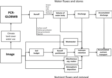
Figure 2.Scheme of the model framework with PCR-GLOBWB and IMAGE and the data flows between the models.
IMAGE provides land cover and soil budgets for N and P and IMAGE–GNM outputs the nutrient delivery to surface water via surface and subsurface runoff (see Sect. 2.4.2 and 2.4.3) (Fig. 2). IMAGE distinguishes grid cells with natural vegetation or agriculture. Within each agricultural grid cell IMAGE computes distributions of seven crop groups that are aggregated in IMAGE–GNM to larger groups (pastoral grassland, grassland in mixed systems, wetland rice, legumes and upland crops). The soil N budget (Nbudget) is calculated
for each of these groups and then aggregated to the level of 0.5◦×0.5◦grid cells for individual years as follows:
Nbudget=Nfix+Ndep+Nfert+Nman−Nwithdr−Nvol, (1)
where Nfixis biological N fixation (kg), Ndepis atmospheric
N deposition (kg), Nfertis application of synthetic N fertilizer
(kg), Nmanis animal manure (kg), Nwithdris N removal from
via crop harvesting, hay and grass cutting, and grass grazed by animals (kg), and Nvol is ammonia (NH3) volatilization
(kg). The N budget is prone to erosion, leaching or denitrifi-cation, or can accumulate in the soil. Following the approach of Bouwman et al. (2013d), the P budget is assumed to de-pend on erosion, and soil accumulation. P inputs for the soil budget are fertilizer and animal manure, and outputs are crop and grass withdrawal.
1 m Soil
Soil nutrient budget
5 m
Shallow groundwater
Water/nutrient flow
Denitrification
Riparian Surface water
Grid cell
50 m
Deep groundwater
Shallow grw by-pass flow Shallow grw flow to riparian Surface runoff
Wastewater/ aquaculture
In-stream retention Atmospheric N deposition
Deep groundwater flow
Soil/aquifer
P sorption
Figure 3.Scheme of the flows of water and nutrients, and retention processes within a grid cell.
P retention in a water body is calculated on the basis of the residence time of the water and nutrient uptake velocity, and subsequently, water and nutrients are transported to downstream grid cells. Discharge is routed to obtain the ac-cumulated water and nutrient flux in each grid cell, through streams, rivers, lakes, wetlands and reservoirs (Fig. 4).
The various submodels for hydrology, spatially explicit nutrient delivery patterns and in-stream retention (Fig. 3), used within IMAGE–GNM are parameterized independently. Furthermore, these parameters are not calibrated in order to better understand the model behavior, identify the lacunae in the data used, and discern the influence of the various pro-cesses considered in the model. Instead, the sensitivity of dif-ferent model outputs to changes in values of input data and model parameters is analyzed in order to explore our model and data.
Although part of the IMAGE framework, GNM can also be used as a stand-alone version, provided that all the in-put data are in the correct format. For example, land cover data and soil N budgets from various modeling groups could be used (Van Drecht et al., 2005; Fekete et al., 2011). Here we use an update of the nutrient data covering the period 1900–2000 presented by Bouwman et al. (2013d). Also, out-put from different hydrological models (e.g., Alcamo et al., 2003; Fekete et al., 2011) could be compared.
IMAGE–GNM is written in Python 2.7 code. The com-plete code is available in the Supplement.
2.2 Hydrology 2.2.1 Water balance
The land surface in PCR-GLOBWB is represented by a top-soil (0.3 m thick or less) and a subtop-soil (1.2 m thick or less). Precipitation falls as rain if air temperature exceeds 0◦C, and
as snow otherwise. Snow accumulates on the surface, and
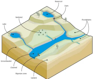
Figure 4.Scheme of the routing of water (with N and P) in a land-scape with streams, rivers, lakes, wetlands and reservoirs; each type of water body within a grid cell is defined by an inflow or discharge, depth and area. Floodplains may be temporarily or permanently flooded.
melt is temperature controlled. Potential evapotranspiration is broken down into canopy transpiration and bare-soil evap-oration, which are reduced to an actual evapotranspiration rate based on soil moisture content. Vertical transport in the soil column arises from percolation or capillary rise, depend-ing on the vertical hydraulic gradient present between these layers.
Precipitation and temperature are from New et al. (2000) and downscaled to daily values using the ERA-40 reanaly-sis (Uppala et al., 2005). Precipitation and temperature were fed directly into the model whereas secondary variables (va-por pressure, wind speed, cloud cover) were used to compute reference potential evapotranspiration using the Penman– Monteith equation according to guidelines of the Food and Agriculture Organization of the United Nations (FAO) (Allen et al., 1998). For the overlapping period 1960–2001, the ac-tual sequence of ERA-40 years was used.
Water drains from the soil column and is delivered as specific runoff to the drainage network, consisting of direct runoff, interflow and base flow. PCR-GLOBWB simulates runoff and converts it to regulated discharge (i.e., includ-ing reservoirs; water extraction is ignored), which is used to simulate waterborne nutrient transport. First, total runoffqtot
(m yr−1) is split into surface runoff (q
sro, m yr−1) and excess
water flow (qeff, m yr−1):
wherefqsrois the fraction of surface runoff with respect to total runoff. Surface runoff represents a large proportion of total runoff in locations where drainage into soils is restricted (e.g., urban areas with sealed surfaces, areas covered with impermeable topsoil, and locations with a steep topography) and is represented as
fqsro=fqsro(slope) fqsro(texture) fqsro(landuse). (3)
Surface runoff is assumed to not be limited (fqsro(texture)=1.0) in soils with very fine topsoil
tex-ture, whereas for loam and sandy loam, and for coarse sand and peat the valuefqsro(texture) is adjusted to 0.75 and 0.25,
respectively.
The slope-runoff classification for unconsolidated sedi-ments is implemented following Bogena et al. (2005):
fqsro(slope)=1−e−0.00617MAX[1,S], (4) whereSis the slope in m km−1. Since this function is
non-linear, fqsro(slope) is the median value of all 90 m×90 m cells within each 0.5◦×0.5◦ grid cell. Land use and soil texture can also influence the surface runoff, and these are implemented via the dimensionless factorsfqsro(texture) and
fqsro(land use), respectively (Velthof et al., 2007, 2009). The
soil map used shows dominant soil texture, and has no bare rock class. In areas with bare rock such as in mountainous regions, slopes are generally steep, and Eq. (4) yields high values forfqsro(slope) and thus forfqsro.
Water stagnation may occur in flat land (slope < 20 m km−1) where soils are saturated based on
the Improved Arno Scheme (Todini, 1996; Hageman and Gates, 2003). Soils that are (semi-) permanently saturated are identified as poorly drained areas and are associated with the occurrence of bogs and peat lands. Also, where percolation at the interface between soil and the groundwater reservoir is impeded (e.g., in the case of permafrost), water can stagnate and drain as topographically driven saturated interflow.
When water infiltrates, it can either flow laterally to ditches and streams or vertically to groundwater. IMAGE– GNM implements two groundwater compartments, follow-ing Van Drecht et al. (2003), De Wit and Pebesma (2001) and De Wit (2001) (Fig. 3). The shallow groundwater sys-tem comprises the top 5 m of the saturated zone where wa-ter is retained over short residence times and can either en-ter the local surface waen-ter at short distances (< 1 m) or infil-trate into the deep groundwater system. A 50 m thick deep groundwater layer (Meinardi, 1994), is located below the shallow groundwater system and significantly contributes to the runoff. The water residence time in the deep groundwa-ter system is much higher than that of the shallow ground-water system, as it flows more slowly at greater depths and drains into the fluvial system at greater distances (> 1 km). IMAGE–GNM assumes no deep groundwater presence (i) in areas with non-permeable, consolidated rocks; (ii) in sed-iments underlying surface waters (rivers, lakes, wetlands,
reservoirs); and (iii) in coastal lowlands (< 5 m above sea level) where (artificial) drainage or a high groundwater level persists (Bouwman et al., 2013a).
The excess water flow qeff (Eq. 5) splits into interflow through the shallow groundwater system (qint, m yr−1) and
deep groundwater runoff (qgwb, m yr−1) as follows:
qeff=(1−fqsro) qtot=qint+qgwb. (5)
The partitioningfqgwb(p)of the excess water flowqeff be-tween these two systems (Fig. 3) is based on the effective porosity (p) of the parent material (Table 1). The deep layer (if present) is assumed to have the same characteristics as the surface layer.
IMAGE-GMN assumes that shallow groundwater inter-flow moves to the fluvial system via riparian zones (Fig. 3), except in (fractions of) grid cells with wetlands, lakes or large streams, where riparian zones are bypassed. Although ripar-ian zones may only account for a small percentage of the drainage basin, they are critical control points for ground-water and N fluxes within many basins (Vidon and Hill, 2006). Riparian zones along small streams have long eco-tone lengths within drainage networks, and may process groundwater N at faster rates than larger nearby water bodies (Bouwman et al., 2013a).
2.2.2 Vegetation and land cover
Vegetation effects are taken into account by partitioning the land surface by fraction into different types. Similarly, spa-tial variations in soil properties can be accounted for by con-sidering effective values for each of these vegetation types. Soil characteristics are assumed to be constant under chang-ing land cover, except for soil total available water capacity (tawc); the relative distribution of tawc varies with chang-ing root depth distributions based on Canadell et al. (1996). All other soil parameters are from the FAO Digital Soil Map of the World (FAO, 1991) and the World Inventory of Soil property Estimates (WISE) data from the International Soil Reference and Information Center (ISRIC) World Soil Infor-mation (Batjes, 1997, 2002). Lithological properties (such as hydraulic conductivity) are derived from a global lithological map (Dürr et al., 2005).
Similar to earlier implementations of PCR-GLOBWB, vegetation parameters are taken from the Olson classification of the global land cover characterization (GLCC) data set with a resolution of 30 arcsec and values assigned using the parameter data set of Hagemann et al. (1999). The parameter-ization is adjusted to the reconstruction of agricultural land cover for 1900–2000 with 5-year time steps derived from the IMAGE model (Bouwman et al., 2013d) based on historical data (Klein Goldewijk et al., 2010, 2011) in order to achieve consistency between the simulated hydrology and imposed land use.
Table 1.Porosity (p), the fraction of excess waterQeffflowing to deep groundwater (fqgwb(p)), half-life of nitrate in groundwater (dt50den),
activation energy (Ea,w) and background P concentration (CPWeath) for various lithological classes.
Lithological classa Porosity (p)b fqgwb(p)c dt50den Ea,w CPWeathd
m3m−3 (–) Year kJ mol−1 g m−3
1. Alluvial deposits 0.15 0.50 2 50 0.0516
2. Loess 0.20 0.67 5 50 0.0256
3. Dunes and shifting sands 0.30 1.00 5 50 0.0790
4. Semi- to unconsolidated sedimentary 0.30 1.00 5 60 0.0248
5. Evaporites 0.20 0.67 5 0 0.0000
6. Carbonated consolidated sedimentary 0.10 0.33 5 0 0.0708
7. Mixed consolidated sedimentary 0.10 0.33 5 60 0.1032
8. Siliciclastic consolidated sedimente 0.10 0.33 1 60 0.0568
9. Volcanic basic 0.05 0.17 5 50 0.0896
10. Plutonic basic 0.05 0.17 5 50 0.0896
11. Volcanic acid 0.05 0.17 5 60 0.0116
12. Complex lithology 0.02 0.07 5 60 0.0645
13. Plutonic acid 0.02 0.07 5 60 0.0224
14. Metamorphic rock 0.02 0.07 5 60 0.0336
15. Precambrian basement 0.02 0.07 5 60 0.0224
aLithological classes as defined by Dürr et al. (2005).bPorosity values from de Wit (1999).cf
qgwb(p)=p/0.3, 0.3 being maximum
porosity.dBackground P concentrations (C
PWeath) were calculated on the basis of Hartmann et al. (2014).eWeathered shales containing
pyrite.
0.5◦×0.5◦ grid cell. To combine this information with the
Olson classification, three separate maps at the original reso-lution of 30 arcsec were created, including (i) Olson classes that were assumed to represent semi-natural vegetation and that were spatially extrapolated per Holdridge life zone (Holdridge, 1967); (ii) Olson classes representing cropland; and (iii) Olson classes representing grassland.
For the reconstructed land cover under the two agricultur-ally managed conditions, i.e., crops and pasture, all 30 arcsec cells within a 0.5◦×0.5◦cell are ranked in order of decreas-ing suitability from 0 to 1. This is achieved by first delin-eating their current extent in the GLCC and ranking on the basis of slope, computed from the Hydro1k database (Verdin and Greenlee, 1996). Next, the adjoining cells are ranked on the basis of the slope parallel distance starting from the de-lineated areas. These rank orders are then normalized, values near zero indicating the most suitable locations, one indicat-ing the poorest locations, and used to match the IMAGE de-rived fractions for each 0.5◦×0.5◦ cell. In this procedure,
cropland has priority, followed by grassland. Any remain-ing areas are subsequently filled with semi-natural vegeta-tion types. On the basis of the resulting patched land cover, the land cover parameterization for PCR-GLOBWB was then derived.
2.2.3 Drainage network
Drainage density is computed from the Hydro1k data set (Verdin and Greenlee, 1996). The drainage network is based on the DDM30 flow direction map of Döll and Lehner (2002) and the lake characteristics taken from the Global Lakes and
Wetlands Database version 1 (GLWD1) product (Lehner and Döll, 2004). Reservoirs are from the Global Reservoir and Dam (GRaND) database (Lehner et al., 2011) and introduced dynamically on the basis of the reported construction year.
The water level in lakes is constant, as the through flow will increase with increasing discharge. The water travel time is determined by the discharge and the volume of the water body. Assuming that flooding occurs once a year and that all river discharge follows the main channel, the travel time in a river with floodplains is determined as follows:
τ= V
Q−Qf
, (6)
whereτ is the travel time (year),V is the volume of the water body (including river bed) (m3),Qis the discharge (m3yr−1)
and Qf is the discharge into the flooded area (m3yr−1).
While the simulated discharge includes the regulating effect of reservoirs, consumptive water use has not been included as it is difficult to identify its source (groundwater, surface water) and to quantify its spatial distribution with certainty.
Water bodies such as lakes and reservoirs can extend over several 0.5◦×0.5◦ grid cells and are included if their
vol-ume exceeds that of the channel within a cell. Where more than one reservoir is located within the same grid cell, they are merged and the combined storage and volume assigned to the dominant reservoir. At the start of the simulation, in 1901, 107 out of a total of 132 reservoirs of the GRaND data set are included as 88 spatially individual water bodies, cor-responding to 78 % of the reported total volume of 16.4 km3.
98 % of the reported total volume of 5848.4 km3. No demand is imposed on the reservoirs and by default they are assigned the purpose of hydropower generation. In absence of pric-ing generation at the global scale (Haddeland et al., 2006; Adam and Lettenmaier, 2008), this results in an operation that maximizes the available potential energy. In this case, this conforms with 75 % of the maximum storage capacity in absence of detailed global data. The remaining 25 % are re-served to buffer inflow for flood control purposes. Reservoir release is linearly scaled to storage when reservoir storage falls below 30 % of the available capacity. This reduced out-flow also results in a realistic, gradual filling of reservoirs after completion of dam construction.
2.3 Nutrient delivery to surface water
Surface and subsurface runoff are calculated from the soil N and P budgets on the basis of the hydrological flows pro-vided by PCR-GLOBWB. Other nutrient sources that are di-rectly delivered to surface water included in IMAGE–GNM are wastewater from urban areas, aquaculture, allochthonous organic matter, weathering and atmospheric deposition. 2.3.1 Nutrients directly delivered to surface water N and P inputs from wastewater for the 20th century are from Morée et al. (2013), and those from freshwater aqua-culture are calculated using the country-scale model esti-mates of Bouwman et al. (2013b) for finfish and Bouwman et al. (2011) for shellfish using data for the period 1950– 2000 from FAO (2013); data indicate that prior to 1950 aqua-culture production was negligible. N and P emissions from aquaculture are allocated within countries using three weigh-ing factors, i.e., population density, presence of surface wa-ter bodies, and mean annual air temperature. For population density, all grid cells with no inhabitants and those with more than 10 000 inhabitants km−2 are excluded; around an
op-timum density of 1000 inhabitants km−2, a steep parabolic
function on the left and less steep on the right are used to calculate the weighing. Lakes, reservoirs, rivers and wetlands have the maximum weight for water bodies, and floodplains and intermittent lakes only half of that; all other types have a weight of zero. Grid cells with mean annual air tempera-ture <0◦C are excluded for aquaculture. The three weighing
factors are combined by multiplication to obtain the overall weight (range=[0,1]). Then all grid cells with overall prob-ability < 10 % are excluded for aquaculture, yielding the map for allocation for all years. Subsequently, the country pro-duction for shellfish and finfish are allocated separately. Grid cells with fish production less than a threshold are excluded for that particular year, and the remaining grid cells are used to allocate the N and P emissions from shellfish and finfish based on the weighing map.
Allochthonous organic matter input to surface water is an important flux in the global C cycle (Cole et al., 2007).
This could be an important source of nutrients, but so far its magnitude has not been investigated. Here, estimates of NPP from IMAGE for wetlands and floodplains are used. Part of annual NPP is assumed to be deposited in the water during flooding, and where flooding is temporary, the litter from pre-ceding periods is assumed to be available for transport in the flood water. The mass ratio of litter to belowground inputs of organic matter ranges from 30 : 70 to 70 : 30 (Vogt et al., 1986; Trumbore et al., 1995); 50 % of total NPP is assumed to end in the surface water. N and P inputs to the water are estimated based on a C : N ratio of 100 and a C : P ratio of 1200 (Vitousek, 1984; Vitousek et al., 1988).
The calculation of P release from weathering is based on a recent study (Hartmann et al., 2014), which uses the ical classes distinguished by Dürr et al. (2005). The litholog-ical classes are available on a 5 by 5 min resolution; hence, the weighted average P concentration within each 0.5◦×0.5◦
grid cell is calculated, and the PRivLoadWeath (kg P yr−1) is
computed as follows:
PRivLoadWeath=10−3CPWeathqtotAgridcellSScorr
exp
−−Ea,w
R
1
K−
1 284
, (7)
whereCPWeath(g m−3) is the background concentration
spec-ified for each lithological class (Table 1) and derived from river runoff data, qtot is the total runoff (m yr−1), A
gridcell
is the land area (m2) in the grid cell considered, SScorr
is a correction factor for soil shielding, Ea,w is the
acti-vation energy (J mol−1) (Table 1), K the local mean an-nual air temperature (Kelvin) andR the molar gas constant (8.3144 J mol−1K−1). The soil shielding correction SS
corris
a correction factor of 0.1 leading to a 90 % reduction for FAO soil units (FAO/Unesco, 1988) Ferralsols, Acrisols, Nitosols, Lixisols, Gleysols (soils with hydromorphic properties) and Histosols (organic soils). For all other soils SScorr=1 (no
re-duction). With this approach, regions with the same lithology but with more precipitation have higher P-weathering losses than regions in dry climates.
Atmospheric N deposition to water bodies is from the en-semble of reactive-transport models for the year 2000 (Den-tener et al., 2006), and the years before that were made by scaling the deposition with grid-based emissions of ammo-nia (Bouwman et al., 2013d). The deposition in floodplains, wetlands and river channels is ignored, because it is already part of the soil N budget, and does not need to be accounted for in periods of flooding.
2.3.2 Surface runoff
IMAGE–GNM distinguishes two surface runoff mobilization pathways for nutrients, i.e., losses from recent nutrient appli-cations in the form of fertilizer, manure or organic matter (Nsro,rec, Psro,rec) (Hart et al., 2004), and a memory effect
in soil nutrient inventories (McDowell and Sharpley, 2001; Tarkalson and Mikkelsen, 2004):
Nsro=Nsro,rec+Nsro,mem. (8)
Estimates of soil loss by rainfall erosion from Cerdan et al. (2010) based on a large database of measurements were used as a basis for calculating Psro,mem and Nsro,mem. The
approach presented by Cerdan et al. (2010) based on slope, soil texture and land cover type were used to estimate coun-try aggregated soil-loss rates for arable land, grassland and natural vegetation. Soil loss from peat soils was assumed to be low (equal to fine texture). These estimates were then ad-justed to obtain the mean erosion loss estimates for Europe (360 t of soil per km2for arable fields, 40 t km−2for
grass-land and 15 t km−2 for natural vegetation). The model was
then applied to all grid cells of the world. For global grass-lands this yields an erosion rate of 60 t of soil per km2, which exceeds the European rate by 50 % due to larger erosivity of grasslands in especially tropical and (semi-)arid climates.
As the model keeps track of all inputs and outputs in the soil P budget, the actual P content can be calculated. The ini-tial P stock for the year 1900 in the top 30 cm is taken from Yang et al. (2013). All inputs and outputs of the soil balance are assumed to occur in the top 30 cm; the model replaces P enriched or depleted soil material lost at the surface by ero-sion with fresh soil material (with the initial soil P content) at the bottom. For N the soil organic C content, which is as-sumed to be constant over time, is used as a basis to calculate N in eroded soil material using land-use-specific C : N ratios (soil C : N for arable land is 12, for grassland 14 and for soils under natural vegetation 14) (based on Brady, 1990; Batjes, 1996; Guo and Gifford, 2002; McLauchlan, 2006). Hence, with changing land use, the N content in soil erosion loss will also change.
Psro,recand Nsro,recare calculated from the N and P input
terms (Eq. 1) on the basis offqsro(Eq. 4). For N the equation is
Nsro,rec=fcalfqsroNinp, (landuse) (9)
where fcal is a correction coefficient of 0.3 to match the N runoff results of the Miterra model (Velthof et al., 2007, 2009).
2.3.3 Subsurface nitrogen removal and delivery Subsurface transport of P is neglected, as P is easily absorbed by soil minerals; leaching of P may occur only in P-saturated soils with long histories of heavy over-fertilization; below the saturated soil layer, P will be absorbed into the minerals occurring there, which are low in P. All the positive values of the soil N budget (Eq. 1) are subjected to leaching. Leaching from the top 1 m of soil (or less for thinner soils) is a fraction of the soil N budget excluding the N lost by surface runoff (fleach,soil; Van Drecht et al., 2003):
Nleach,soil=fleach,soil(Nbudget−Nsro), (10)
wherefleach,soilis
fleach,soil= [1−MIN[(fclimate+ftext+fdrain
+fsoc),1]]flanduse. (11)
The fraction of N lost by denitrification (fden,soil)
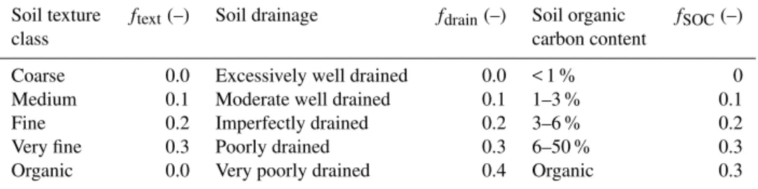
comple-mentsfleach,soil(fden,soil=1−fleach,soil).ftext,fdrainandfsoc
represent factors that address the soil texture, aeration and soil organic carbon (C) content, respectively (Table 2). Fine-textured soils are more susceptible to reach and maintain anoxia, which favors denitrification, as they are characterized by higher capillary pressures and hold water more tightly than sandy soils. Denitrification rates tend to be higher in poorly drained than in well-drained soils (Bouwman et al., 1993). The soil organic C content is used as a proxy for the C supply, which can have a direct impact on the soil oxy-gen concentrations.flanduseis the land use effect on leaching,
where arable land has a value of 1, and grassland and natural vegetation a value of 0.36 (Keuskamp et al., 2012).
The factorfclimate(–) combines the effects of temperature, water residence time, and NO−3 in the root zone on denitrifi-cation rates.fclimateis the product of the temperature effects
on denitrification (fK, –) and the mean annual residence time
of water and NO−3 in the root zone (Tr,so, yr):
fclimate=fKTr,so. (12)
The temperature effectfK follows the Arrhenius equation
(Firestone, 1982; Kragt et al., 1990; Shaffer et al., 1991):
fK=7.94×10¹²exp
−Ea,d
R K
, (13)
whereEa,dis the activation energy (74830 J mol−1),K the
mean annual temperature (Kelvin) andR is the molar gas constant (8.3144 J mol−1K−1).Tr,sois calculated via:
Tr,so=
tawc
qeff , (14)
where tawc (m) is the total available water capacity for the top 1 m (or less if thinner) of soil andqeff is described in
Eq. 5. Based on the negligible retardation of NO−3, the water and NO−3 residence times are assumed to be the same. Soils used for agricultural crops in dry regions with Tr,so< 1
re-ceive aTr,sovalue of 1.0 assuming that irrigation is required
to grow crops in these locations.
Arid regions under grassland or natural vegetation have long residence times according to Eq. (14), and results in values offclimateandfden,soilequal 1, implying that
Table 2.Denitrification fractions for soil texture, soil organic carbon and soil drainage.
Soil texture ftext(–) Soil drainage fdrain(–) Soil organic fSOC(–)
class carbon content
Coarse 0.0 Excessively well drained 0.0 < 1 % 0
Medium 0.1 Moderate well drained 0.1 1–3 % 0.1
Fine 0.2 Imperfectly drained 0.2 3–6 % 0.2
Very fine 0.3 Poorly drained 0.3 6–50 % 0.3
Organic 0.0 Very poorly drained 0.4 Organic 0.3
Source: Van Drecht et al. (2003).
Schlesinger, 1990), but it is clear that only a negligible part of N surpluses in arid climates is lost by denitrification. Denitri-fication was thus neglected from the fate of N surplus in soils receiving an annual precipitation of < 3 mm and overlain with grasslands and natural vegetation. For the year 2000, N sur-plus in the 3100 Mha of global arid lands was 20 Tg.
The N concentrationCNin the excess water leaching from
the root zone (depth z=0) is represented by the ratio of leached N overqeff(Eq. 5):
CN(z=0)=Nleach
qeff
. (15)
The groundwater N concentration varies according to the his-torical year of infiltration into the saturated zone and the den-itrification (including anammox) during groundwater advec-tion (Böhlke et al., 2002; Van Drecht et al., 2003). The time available for denitrification is represented by the mean travel timeTr,aq, which is the ratio of the specific groundwater
vol-ume and the water recharge:
Tr,aq(t )=MIN
p D
qinflow(t )
,1000
, (16)
where D is aquifer thickness (m) and can either be for shallow groundwater (Dsgrw=5 m) or for deep groundwa-ter (Ddgrw=50 m) following Meinardi (1994).qinflowis ei-ther the shallow groundwater recharge (qint, m yr−1) or deep
groundwater recharge, (qgwb, m yr−1). The vertical drainage
of the shallow groundwater feeds the deep groundwater (Fig. 3). The vertical flow distribution for the shallow system is uniform; therefore, the travel time can be equated to the mean travel time. In contrast, travel times for lateral flows to the fluvial system vary considerably. The travel time distribu-tion for lateral flow in a vertical cross secdistribu-tion is represented by Meinardi (1994):
gage(z)= −Tr,aqln(1−(z/D)), (17)
wheregage(yr) is the age of groundwater at a specific depth,
andz(m) is the depth in the aquifer (i.e.,z=0 at the top of the aquifer andz=Dat the bottom of the aquifer).
Denitrification takes place during transport in the shal-low system along the various fshal-low paths in a homogeneous
and isotropic aquifer, drained by parallel rivers or streams. IMAGE–GNM simulates the effects of denitrification in N concentrations at timetand depthz(CN(t, z)) through a
first-order degradation reaction, leading to an exponential decay Eq. for the nitrogen concentration:
CN(t, z)=CN t−gage(z),0e−kgage(z), (18)
wheret is time and the decay ratekis obtained via the half-life of nitrate (dt50den) due to denitrification:
k= ln(2)
dt50den
. (19)
Lithology can have a direct effect on denitrification, and thus
dt50den (Dürr et al., 2005). Siliciclastic material exhibits
lowdt50den values of 1 yr−1, whereas alluvial material has
dt50denvalues of 2 yr−1and all other lithology classes have
adt50den value of 5 yr−1(Table 1). The N concentration in
water percolating to deep groundwater represents the outflow from shallow groundwater. IMAGE-GMN assumes that den-itrification is absent in deep groundwater. Although denitrifi-cation could occur in organic matter- and/or pyrite-rich deep aquifers, denitrification measurements in the literature have a bias toward high rates (Green et al., 2008), which makes their global assessment difficult.
Following Beusen et al. (2013), nitrogen transported through submarine groundwater discharge (SGD) is ex-cluded from the delivery to rivers and other water bodies. This assumption is justified, since, only 10 % of the gridded map could contribute to SGD. The remaining aquifer dis-charge in the grid box goes towards streams and rivers.
While urban areas can have an effect in the N loss to the environment (e.g., Foppen, 2002; Wakida and Lerner, 2005; Van den Brink et al., 2007; Nyenje et al., 2010), the total ur-banized land represents 0.3 % of the total land area (Angel et al., 2005), and thus it is neglected from the model. The median NH4 concentration in groundwater of 25 European
aquifers is 0.15 mg L−1(Shand and Edmunds, 2008), which
represents a small part (0.7–1.2 %) of the nitrogen concen-tration (EEA, 2012), and thus NH4 in groundwater is also
2.3.4 N transport and removal in riparian zones Modeling geochemical processes in riparian zones require a detailed hydrological and geographical information at very high spatial scales, since, even at 0.1 km resolution, the to-pography of the riparian area cannot be adequately assessed (Vidon and Hill, 2006). IMAGE–GNM therefore uses a con-ceptual approach.
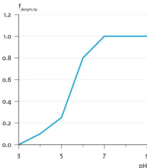
In riparian zones, denitrification rates depend highly on the local pH (Knowles, 1982; Simek and Cooper, 2002), temper-ature, water saturation, NO−3 availability and soil organic car-bon availability. Previous laboratory studies of pure cultures have shown that denitrification is maximized at a pH of 6.5 to 7.5, and decreases at both low (below 4) and high (above 10) pH values (Van Cleemput, 1998; Van den Heuvel et al., 2011).
As with soil denitrification, riparian zone denitrification is calculated using dimensionless reduction factors and is based on the characteristics of the groundwater flow, soil and cli-mate. Heterotrophic denitrification is assumed to be highest at pH > 7 (Van den Heuvel et al., 2010). A pH reduction fac-torfdenpH,ripis then used to reduce the value with decreasing
pH, such thatfdenpH,rip=1 at pH > 7 and 0 at pH < 3 (Fig. 5).
Nden,rip=fden,ripNin, (20)
where Nin is the nitrogen that enters the riparian zone from
the shallow groundwater.
fden,rip=MIN(fclimate+ftext+fdrain
+fsoc) ,1
fdenpH,rip, (21)
wherefclimate is the product offK (Eq. 13) and the water
(and NO−3) travel time through the riparian zone (Tr,rip).Tr,rip
depends on the thickness of the riparian zone (Drip≤0.3 m,
depending on the soil thickness), on the available water ca-pacity for the top 1m of the riparian zone (tawc), and on the flow of water entering the riparian zone from the shallow groundwater (qint) :
Tr,rip=
Driptawc
qint
. (22)
2.4 In-stream nutrient retention
Three processes contribute to N retention, i.e., denitrification, sedimentation and uptake by aquatic plants. Denitrification is generally the major component of N retention (Saunders and Kalff, 2001). P is removed by sedimentation and sorption by sediment (Reddy et al., 1999). Retention in a grid cell is calculated as a first-order approximation according to
R=1−exp
v
f,E
HL
, (23)
Figure 5.Reduction fraction (fdenpH,rip) of riparian denitrification
as a function of soil pH modified from Bouwman et al. (2013a).
whereR is the fraction of the nutrient load that is removed (–),vf is the net uptake velocity (m yr−1),Eis the nutrient
considered (N or P), andHL is the hydraulic load (m yr−1)
obtained from
HL=D
τ , (24)
whereDis the depth of the water body (m),τis the residence time (yr) andτis calculated from the volumeV (m3) of the water body and the dischargeQ(m3yr−1):
τ=V
Q (25)
for all water bodies except for river channels and floodplains where the dischargeQis reduced by the water volume in the floodplains (see Eq. 6). In this approach hydrological (de-fined byHL) and biological and chemical factors (defined
byvf) controlling retention are isolated, assuming first-order
kinetics is applicable (i.e., areal uptake changes linearly with concentration).
Net uptake velocity is different for each elementE (N or P). For N, the basic value for all water body types of 35 m yr−1taken from (Wollheim et al., 2006, 2008a) is mod-ified based on temperature and N concentration:
vf,N=35f (t ) f (CN) , (26)
wheret is annual mean temperature (◦C) and CN is the N
concentration in the water.f (CN) describes the effect of
from a value of 7.2 at CN=0.0001 mg L−1 to 1 for C
N=
1 mg L−1, a further decrease to 0.37 for C
N=100 mg L−1
and constant at higher concentrations. The temperature effectf (t )is calculated as
f (t )= ∝t−20(t−20), (27)
whereα=1.0717 for N (following Wollheim et al., 2008a and references therein) andα=1.06 for P (following Marcé and Armengol, 2009).
For P, the basic value for vf of 44.5 m yr−1 taken from
Marcé and Armengol (2009) is used for all water body types, with a modification based on temperature:
vf,P=44.5f (t ) . (28)
The drainage network of PCR-GLOBWB represents streams and rivers of Strahler order (Strahler, 1957) 6 and higher. The parameterization of lower-order streams follows the ap-proach presented by Wollheim et al. (2008b). A globally uni-form subgrid river network is included for all grid cells with-out lakes or reservoirs. It is assumed that PCR-GLOBWB has one river of order 6 in each grid cell, and all lower-order rivers are lacking. The river network is then defined on the basis of stream length and basin area of the first-order river. The mean length ratioRL(–) is used to calculate the stream length of the next higher order the river according to
Ln=L1RL(n−1), (29)
with Ln being the stream length of order n (km); L1=
1.6 km. The drainage area ratio Ra (–) is used to calculate the basin area for higher-order stream as follows:
An=A1Ra(n−1), (30)
whereAnis basin area of ordernin km2;A1=2.6 km2. With
the stream number ratio Rb (–) the number of lower-order
streams is calculated as
Rn=R(6
−n)
b , (31)
withRnbeing the number of streams of ordernin this grid
cell;Rb=4.5. The discharge for each stream is calculated
with the runoff (q):
Qn=qAnCQ, (32)
with the discharge of stream ordern(Qn) in m3s−1, runoff in
mm yr−1andC
Q the unit conversion (CQ=1000/(3600×
24×365)). The midpoint discharge of a stream length of or-dernis calculated as
Qmid,n=Qn+0.5Qn−1. (33)
The width of the stream of order n is calculated as
Wn=A(Qmid,n)B, (34)
whereWn=width (m),Ais a constant (A=8.3 m) and
co-efficientB=0.52. It is now possible to calculate the hydro-logic load (HL) and thus the retention of the stream according to
HL=
CQ1Qmid,n
LnWnCQ2
, (35)
withCQ1being the conversion from seconds to years (CQ1=
3600×24×365),CQ2the conversion from km to m (1000)
andHLin m yr−1. The local diffuse load in a grid cell is
spa-tially uniformly distributed over the streams. Here, the frac-tion of the total stream length per order is used to calculate the distribution of the load. The direct load is allocated to stream-ordernas follows:
Fd,n=
RnLn
P6
i=1RiLi
, (36)
whereFd,nis the fraction of the total load, which is direct
in-put for streams of ordern. The pathway of the outflow of the streams is determined according to a matrixTi,jrepresenting
the fraction of the outflow of stream-orderito stream-order
j, wherebyTi,j =0.0 fori≥j. Fori<j,Ti,j is calculated
as follows: Ti,j=
RjLj
P6
k=i+1RkLk
. (37)
The calculation of the retention is performed for each stream order, starting with ordern=1, and is identical to the calcu-lation of the PCR-GLOBWB schematization. The load of a stream is the sum of the direct load and the sum of the out-flow from lower-order streams.
2.5 Data analysis
For the comparison of observations for individual monitor-ing stations or ad hoc measurements in rivers and simulated concentrations of river water, we use the root mean squared error (RMSE) expressed as a percentage. RMSE is calculated as follows:
RMSE=100
O
s
Pn
i=1(Oi−Mi)2
n , (38)
whereOis the mean of the observations,Oiis observationi,
Mi is the simulated valueiandnis the number of data pairs.
We consider values of 50 % acceptable in view of the global scale of the model.
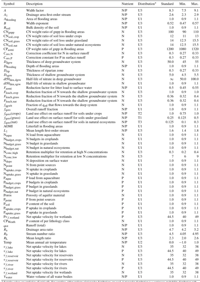
Table 3.Model parameters included in the sensitivity analysis, their symbol and description, for which nutrient it is used, and the standard, minimum, mode and maximum value considered for the sampling procedure. Parameters are listed in alphabetical order of their symbol.
Symbol Description Nutrient Distribution∗ Standard Min. Max.
A Width factor N/P U3 8.3 7.5 9.1
A1 Drainage area first-order stream N/P U3 2.6 2.3 2.9
Aflooding Area of flooding areas N/P U1 1.0 0.9 1.1
B Width exponent N/P U3 0.52 0.47 0.57
Bsoil Bulk density of the soil N/P U1 1.0 0.9 1.1
CNgnpp CN weight ratio of gnpp in flooding areas N U3 100 90 110
CNsoil,crop CN weight ratio of soil loss under crops N U3 12 11 13
CNsoil,grass CN weight ratio of soil loss under grassland N U3 14 12.5 15.5
CNsoil,nat CN weight ratio of soil loss under natural ecosystems N U3 14 12.5 15.5
CPaomi CP weight ratio of gnpp in flooding areas P U3 1200 1080 1320
Csro,N Correction coefficient for N in surface runoff N U3 0.3 0.27 0.33
Csro,P Correction constant for P in surface runoff P U3 0.3 0.27 0.33
Ddgrw Thickness of deep groundwater system N U3 50.0 45 55
Dflooding Depth of flooding areas N/P U1 1.0 0.9 1.1
Drip Thickness of riparian zone N U3 0.3 0.27 0.33
Dsgrw Thickness of shallow groundwater system N U3 5.0 4.5 5.5
dt50den,dgrw Half-life of nitrate in deep groundwater N U3 ∞ 50.0 100.0
dt50den,sgrw Half-life of nitrate in shallow groundwater N U1 1.0 0.9 1.1
Faomi Reduction factor for litter load to surface water N/P U1 0.5 0.45 0.55
Fleach,crop Reduction fraction of N towards the shallow groundwater system N U3 1.0 0.9 1.0
Fleach,grass Reduction fraction of N towards the shallow groundwater system N U3 0.36 0.32 0.4
Fleach,nat Reduction fraction of N towards the shallow groundwater system N U3 0.36 0.32 0.4
fqgwb Fraction ofqeffthat flows towards the deep system N U1 1.0 0.9 1.1
fqsro Overall runoff fraction N/P U1 1.0 0.9 1.1
fqsro(crops) Land use effect on surface runoff for soils under crops N/P T2 1.0 0.75 1.0
fqsro(grass) Land use effect on surface runoff for soils under grassland N/P T1 0.25 0.125 0.5
fqsro(nat) Land use effect on surface runoff for soils in natural ecosystems N/P T3 0.125 0.1 0.3
AOMI Litterfall in flooding areas N/P U1 1.0 0.9 1.1
L1 Mean length first-order stream N/P U3 1.6 1.4 1.8
Naqua N load from aquaculture N U1 1.0 0.9 1.1
Nbudget,crops N budgets in croplands N U1 1.0 0.9 1.1
Nbudget,grass N budget in grasslands N U1 1.0 0.9 1.1
Nbudget,nat N budget in natural ecosystems N U1 1.0 0.9 1.1
Nconc,high Retention multiplier for retention at high N concentrations N U3 0.3 0.2 0.4
Nconc,low Retention multiplier for retention at low N concentrations N U3 7 6 9
Ndepo N deposition on surface water N U1 1.0 0.9 1.1
Npoint N from point sources N U1 1.0 0.9 1.1
Nuptake,crops N uptake in croplands N U1 1.0 0.9 1.1
Nuptake,grass N uptake in grasslands N U1 1.0 0.9 1.1
Paqua P load from aquaculture P U1 1.0 0.9 1.1
Pbudget,crops P budgets in croplands P U1 1.0 0.9 1.1
Pbudget,grass P budget in grasslands P U1 1.0 0.9 1.1
Pbudget,nat P budget in natural ecosystems P U1 1.0 0.9 1.1
Poros Porosity of aquifer material N U1 1.0 0.9 1.1
Ppoint P from point sources P U1 1.0 0.9 1.1
Psoil P content of the soil P U1 1.0 0.9 1.1
Puptake,crops P uptake in croplands P U1 1.0 0.9 1.1
Puptake,grass P uptake in grasslands P U1 1.0 0.9 1.1
Pvf,wetland Net uptake velocity for wetlands P U3 44.5 40 49
CPWeath P content of per lithology class N U1 1.0 0.9 1.1
qtot Runoff (total) N/P U1 1.0 0.9 1.1
Ra Drainage area ratio N/P U3 4.7 4.2 5.2
Rb Stream number ratio N/P U3 4.5 4.05 4.95
RL Mean length ratio N/P U3 2.3 2.0 2.6
Temp Mean annual air temperature N/P U2 0.0 −1.0 1.0
vf,lake Net uptake velocity for lakes N U3 35 32 38
vf,lake Net uptake velocity for lakes P U3 44.5 40 49
vf,reservoir Net uptake velocity for reservoirs N U3 35 32 38
vf,reservoir Net uptake velocity for reservoirs P U3 44.5 40 49
vf,river Net uptake velocity for rivers N U3 35 32 38
vf,river Net uptake velocity for rivers P U3 44.5 40 49
vf,wetland Net uptake velocity for wetlands N U3 35 32 38
Vwater Water volume of all water bodies N/P U1 1.0 0.9 1.1
∗Samples values are applied to all grid cells. For sampling, either uniform of triangular distributions are used. A triangular distribution is a continuous probability distribution with
lower limita, upper limitband modec, wherea≤c≤b. The probability to sample a point depends on the skewness of the triangle. In the case ofdt50den,dgrw,ac=bc, and probability to sample a point on the left and right hand side ofcis the same. In other cases, for example,fqsro(crops) is a fraction (range=[0,1]), with standard value of 1.0. To achieve a high probability to sample close to 1.0, the triangle is designed withb=1andcis close to 1. For some of the above distributions the expected value is not equal to the standard. Since the calculatedR2for all output parameters exceeds 0.99, this approach for analyzing the sensitivity is still valid. The distributions used are U1. Uniform; values are multipliers for
stratified sample method based on subdividing the range of each of thekparameters into disjunct equiprobable intervals or runs (Num). By sampling one value in each of the Num intervals according to the associated distribution in this in-terval, Num sampled values are obtained for each parameter. Num was 500 for P and 750 for N.
The sampled values for the first model parameter are ran-domly paired to the samples of the second parameter, and these pairs are subsequently randomly combined with the samples of the third source, and so forth. This results in an LHS consisting of Num combinations of kparameters. The parameter space is thus representatively sampled with a lim-ited number of samples.
The uncertainty contributions of each input parameter (Xi)
can be further assessed by combining LHS with linear re-gressions with respect to the model outputs (Yi) via Saltelli
et al. (2000, 2004):
Y =β0+β1X1+β2X2· · · +βnXn+e, (39)
whereβiis the so-called ordinary regression coefficient ande
is the error of the approximation. The linear regression model can be evaluated using the coefficient of determination (R2), which represents theY variation as explained byY−e.βi
de-pends on the scale and dimension ofXi, the sensitivity study
can be normalized by rescaling the regression equation using of the standard deviations forY andX(σY andσXi,
respec-tively) and calculating the standardized regression coefficient (SRCi):
SRCi=βi
σXi
σY
. (40)
SRCican take values in the interval [−1,1]. SRC is the
rela-tive change1Y /σY ofY due to the relative change1Xi/σXi of the parameter Xi considered (both with respect to their
standard deviation σ). Hence, SRCi is independent of the
units, scale and size of the parameters, and thus sensitivity analysis comes close to an uncertainty analysis. A positive SRCi value indicates that increasing a parameter value will
cause an increase in the calculated model output, while a negative value indicates a decrease in the output considered caused by a parameter increase.
The sum of squares of SRCivalues of all parameters equals
the coefficient of determination (R2), which for a perfect fit equals 1. Hence, SRC2i/R2yields the contribution of param-eterXi toY. For example, a parameterXi with SRCi=0.1
adds 0.01 or 1 % toY in caseR2equals 1.
3 Analysis of the model results
3.1 Comparison with measurement data
We first compared the IMAGE–GNM model results with ob-served concentrations for two stations in the rivers Rhine and
Meuse and at 11 stations in the Mississippi, USA (see Sup-plement). Stations near the river mouth (Lobith at the Rhine, Eysden at the Meuse, and St. Francisville, Louisiana, for the Mississippi) are shown first. The latter station was selected for comparison due to its widespread use in literature, for ex-ample by the US Geological Survey analysis of water qual-ity (US Geological Survey, 2009). The measured concen-trations were first aggregated to annual discharge-weighed concentrations, whereby for the US data years with < 6 ob-servations were excluded. The model performance for the river Rhine for N concentrations (RMSE=15 %) is better than for the Meuse and Mississippi (Fig. 6a, b, d, e, g, h). IMAGE–GNM overestimates N concentrations in the river Meuse (RMSE=31 %) in almost all years; the model under-estimates N concentrations in the early 1980s for the Mis-sissippi, while its performance is better from the second half of the 1980s (RMSE for Mississippi=23 %). P concen-trations in the Mississippi are consistently underestimated (RMSE=51 %) (Fig. 7a, b, d, e, g, h). P concentrations are overestimated in the Rhine in all years with data, although the declining trend is well captured (RMSE=28 %). The mod-eled P concentrations are close to observations in the Meuse, with deviations in both directions (RMSE=36 %).
The residues (observation minus simulation) for the ob-served vs. simulated concentrations of N and P (Figs. 6c and 7c) in the Mississippi show a very clear trend from overesti-mation at low concentrations to underestioveresti-mation at high con-centrations. The residues show a trend in the Rhine, with a slight increase along with increasing concentrations (Figs. 6f and 7f). The Meuse also shows such trends, although less clear. For P the residue increases with increasing concentra-tion, and for N the opposite occurs (Figs. 6i and 7i).
Since the deviations from observed concentrations can stem from errors in the hydrology, we compared the simu-lated vs. observed discharges (Fig. 8). Results for the Mis-sissippi (Fig. 8a) show a good agreement but with overesti-mation in most years. While the RMSE is 19 % for the Mis-sissippi, there is no consistent trend between residue and dis-charge, indicating no systematic error (Fig. 8b). The RMSE for the discharge of the Rhine is 14 %, with a consistent un-derestimation by the model (Fig. 8c), and the residues show a clear increase with observed discharge (Fig. 8d), indicating a systematic error in the model. For the Meuse, the RMSE for the discharge is 23 %, the discharge seems to be over-estimated (Fig. 8e), and there is only a small trend between discharge and residue (Fig. 8f).
over-0 1 2 3 4
0 1 2 3 4
O
b
se
rv
ed
N
c
o
n
cen
tr
a
i
o
n
m
g
N
l
-1
Simulated N concentraion mg N l -1
Mississippi
y = 1.051x - 2.243 R² = 0.7628
-1 -0.5 0 0.5 1 1.5
0 0.5 1 1.5 2 2.5 3 3.5
R
e
si
d
ue
N
c
o
n
ce
n
tr
a
i
o
n
m
g
N
l
-1
Observed N concentraion mg N l -1
Mississippi
(a) (b) (c)
(d) (e) (f )
(g) (h) (i)
Figure 6.Comparison of modeled (black line) and measured (light blue, and aggregated yearly) discharge-weighed concentrations of total N
in the rivers Mississippi(a–c), Rhine(d–f)and Meuse(g–i). Panels on the left are comparisons over time; panels in the center represent plots
of simulations vs. observations with a 1 : 1 line, and panels on the right are the concentrations vs. the residues (observation minus simulation) with a regression line.
estimated; simulated P concentrations are in good agreement with observations, while N concentrations are overestimated; hence, there is no clear connection between the model errors in discharge and nutrients.
We also investigated the model performance for 10 more stations in various states within the Mississippi River basin (Table 4). These stations along with the St. Francisville sta-tion form the monitoring network for nine subbasins in the Mississippi (US Geological Survey, 2007). The plotted data for all 11 stations in Mississippi River basin are available as separate graphs in the Supplement. The model performance is acceptable (RMSE < 50 %) for eight stations for N con-centrations and five stations for P concon-centrations. There are some stations where the model poorly simulates the N con-centrations such as Arkansas River and Red River (Table 4). Such high RMSE values do not occur for P. In general, sim-ulated P concentrations are closer to observed values than N concentrations.
One of the reasons for poor agreement is the large fluctu-ation of discharge, load and concentrfluctu-ation at some stfluctu-ations. Apparently, these peaks are associated with periods of high rainfall. We do not know if these peak values represent the
full period of the measurement interval. For example, a peak value that represents 2 months (in the case there are six mea-surements per year) also yields a peak in the aggregated an-nual value. However, it is not known if this peak actually rep-resents 1 day (with a much lower aggregated annual value) or 2 months. In contrast to St. Francisville, P concentrations (and N concentrations) at the other stations are not consis-tently underestimated or overestimated. Furthermore, at this level of comparison, the spatial data for land use and wastew-ater discharge locations in urban areas may not be realistic. For example, our wastewater discharge occurs in all grid cells with urban population, while in reality discharge takes place in discrete locations such as wastewater treatment plants.
A further performance test involves a direct comparison between aggregated data and model results for a large num-ber of European rivers (see Supplement) (European Envi-ronment Agency, 2013). This data set includes monitor-ing data at different stations for 125 rivers, 49 for N and 76 for P. River basins with less than four grid cells, of
0 0.1 0.2 0.3 0.4 0.5 0.6 0.7 0.8 0.9 Co n ce n tr a i o n in m g P L -1
Phosphorus concentraion Mississippi
Observaion Year observaion Simulated 0 0.1 0.2 0.3 0.4
0 0.1 0.2 0.3 0.4
O b se rv ed P co n cen tr a i o n m g P l -1
Simulated P concentraion mg P l -1
Mississippi y = 0.804x - 0.0698 R² = 0.9105
0 0.05 0.1 0.15 0.2 0.25
0 0.05 0.1 0.15 0.2 0.25 0.3 0.35
R e si due P co n cen tr a i o n m g P l -1
Observed P concentraion mg P l -1
Mississippi 0 0.2 0.4 0.6 0.8 1 1.2 1.4 1.6 1.8 2 Co n ce n tr a i o n in m g P /l
Phosphorus concentraion Rhine
Observaion Year observaion Simulaion
(a) (b) (c)
(d) (e) (f )
(g) (h) (i)
Figure 7.Comparison of modeled (black line) and measured (light blue, and aggregated yearly) discharge-weighed concentrations of total P
in the rivers Mississippi(a–c), Rhine(d–f)and Meuse(g–i). Panels on the left are comparisons over time; panels in the center represent plots
of simulations vs. observations with a 1 : 1 line, and panels on the right are the concentrations vs. the residues (observation minus simulation) with a regression line.
basins with 4–10 grid cells also suffer the problem of poor spatial data. Measurements for some stations were removed from the data set as outliers (Table S1). Results for all mea-surements show a coefficient of determination of 0.59 and RMSE of 124 % for N (n=709) and 0.58 and RMSE of 184 % for P (n=1010) (Fig. 9a and b). Results show rea-sonable coefficients of determination (r2) of 0.79 and RMSE of 112 % for P and 0.55 and RMSE of 95 % for N (Fig. 9c and d). The average of all measurements for N and P is slightly lower than the simulated concentrations (0.16 vs. 0.25 mg P L−1and 1.25 vs. 1.78 mg N L−1). The mean of
ob-servations and model values over the monitoring period for each station showed good agreement (Fig. 9e and f). There is also good agreement between model and data for the mean for all stations for each year with deviations never exceeding 1 mg N L−1and 0.2 mg P L−1(Fig. 9e and f). It is clear that the model has problems when modeling individual stations in small rivers in the database. The plotted data for all sta-tions in the European rivers (available as separate graphs in the Supplement) show that the model results for the Danube, for example, are in good agreement with observations for two stations. Most simulated concentrations are within a factor of
2 of the observed concentrations in the EEA database (EEA, 2012).
Our model results also show a fair agreement with the vali-dation data set for the early 1990s for total N collected by Van Drecht et al. (2003) (Fig. 10). Modeled total N concentrations for the Amazon for the early to mid-1980s (0.7–0.9 mg L−1)
are close to measured values (0.4–0.5), and results for total P (0.07 mg L−1) are also close to observations (0.06 mg L−1)
(Forsberg et al., 1988; Meybeck and Ragu, 1995).
These comparisons of our model output with data at var-ious aggregation levels show that IMAGE–GNM based on three calibrated submodels (hydrology, nutrient input and in-stream removal) performs very well without any tuning of the overall, integrated model. We have deliberately chosen to not further tune the model so that we can identify its shortcom-ings. Further improvement of model performance requires a sensitivity analysis.
3.2 Model sensitivity
(f ) (e)
(d) (c)
0 100 200 300 400 500 600 700 800
0 100 200 300 400 500 600 700 800
O
b
se
rv
e
d
y
e
ar
ly
d
is
ch
ar
g
e
k
m
3y
r
-1
Simulated yearly discharge km3yr -1
Mississippi y = 0,1557x - 133,91
R² = 0,0785
-200 -150 -100 -50 0 50 100
0 100 200 300 400 500 600 700
R
e
si
d
u
e
y
e
ar
ly
d
is
ch
ar
g
e
k
m
3y
r
-1
Observed yearly discharge km3yr -1
Mississippi
(a) (b)
Figure 8.Comparison of simulated and observed annual discharge (left-hand graphs with 1 : 1 lines) and residues (observation minus
simu-lation) vs. observation (right-hand graphs with regression lines) for Mississippi(a, b), Rhine(c, d)and Meuse(e, f).
significant and have an SRC value > 0.2 or <−0.2 (parame-ters that add > 4 % to the delivery, retention or river export). Results presented in Tables 5 and 6 show that the sensitiv-ity of N delivery, retention and river export for the year 2000 differs from that of P in many aspects.
Total runoff (qtot; Eq. 5) is significant for retention and
river export of both N and P; runoff largely determines all transport pathways and flows of N (runoff, leaching, ground-water flow and also in-stream retention), and it determines P runoff, the major transport pathway for P. The soil N budget in natural ecosystems and arable land (Nbudget,crops;
Nbudget,nat; Eq. 1) are important factors for the N delivery,
but not for the retention and river export. For P the soil bud-gets are less important, because soil P content (Psoil) and bulk
density (Bsoil) govern the runoff of P more than the budget; actually, soil P content is actually a result of the long-term soil P budget.
Our model results suggest that allochthonous organic mat-ter input to stream is an important but uncertain nutri-ent source. The factors determining the allochthonous or-ganic matter input of N to streams and rivers (flooded area,
Aflooding; litterfall, AOMI; its reduction factor for litterfall,
FAOMI; and its C : N ratio) are similarly important for the
delivery and river export of N. For P both the parameters determining allochthonous inputs and weathering (CPWeath;
Eq. 7) are not significant nor important, as the biomass from litterfall contains only small amounts of P and because the anthropogenic sources are dominant.
For the modeling of river retention, the sensitivity analy-sis for a range of parameters shows that net uptake veloc-ity (Vf,river,N; Vf,river,P; Eqs. 23, 26, 28) and mean length
ratio (RL; Eq. 29) are important for retention and river
ex-port for both N and P, and logically not for nutrient deliv-ery. The assumption that N retention depends on N concen-trations (Nconc,low; Eq. 26) is significant in all years for the
retention and river export. Temperature (Temp; Eq. 27) is im-portant for retention of P, and for retention and river export of N.