www.geosci-model-dev.net/10/127/2017/ doi:10.5194/gmd-10-127-2017
© Author(s) 2017. CC Attribution 3.0 License.
Calibrating a global three-dimensional biogeochemical
ocean model (MOPS-1.0)
Iris Kriest1, Volkmar Sauerland2, Samar Khatiwala3, Anand Srivastav2, and Andreas Oschlies1
1GEOMAR Helmholtz-Zentrum für Ozeanforschung Kiel, Düsternbrooker Weg 20, 24105 Kiel, Germany
2Institut für Informatik, Christian-Albrechts-Universität zu Kiel, Christian-Albrechts-Platz 4, 24098 Kiel, Germany 3Department of Earth Sciences, University of Oxford, South Parks Road, Oxford OX1 3AN, UK
Correspondence to:Iris Kriest ([email protected])
Received: 4 July 2016 – Published in Geosci. Model Dev. Discuss.: 18 July 2016 Revised: 8 December 2016 – Accepted: 14 December 2016 – Published: 9 January 2017
Abstract. Global biogeochemical ocean models contain a variety of different biogeochemical components and often much simplified representations of complex dynamical in-teractions, which are described by many (≈10 to ≈100) parameters. The values of many of these parameters are em-pirically difficult to constrain, due to the fact that in the mod-els they represent processes for a range of different groups of organisms at the same time, while even for single species pa-rameter values are often difficult to determine in situ. There-fore, these models are subject to a high level of parametric uncertainty. This may be of consequence for their skill with respect to accurately describing the relevant features of the present ocean, as well as their sensitivity to possible environ-mental changes.
We here present a framework for the calibration of global biogeochemical ocean models on short and long timescales. The framework combines an offline approach for transport of biogeochemical tracers with an estimation of distribution algorithm (Covariance Matrix Adaption Evolution Strategy, CMA-ES). We explore the performance and capability of this framework by five different optimizations of six bio-geochemical parameters of a global biobio-geochemical model, simulated over 3000 years. First, a twin experiment explores the feasibility of this approach. Four optimizations against a climatology of observations of annual mean dissolved nu-trients and oxygen determine the extent to which different setups of the optimization influence model fit and parame-ter estimates. Because the misfit function applied focuses on the large-scale distribution of inorganic biogeochemical trac-ers, parameters that act on large spatial and temporal scales are determined earliest, and with the least spread. Parameters
more closely tied to surface biology, which act on shorter timescales, are more difficult to determine. In particular, the search for optimum zooplankton parameters can benefit from a sound knowledge of maximum and minimum parameter values, leading to a more efficient optimization. It is encour-aging that, although the misfit function does not contain any direct information about biogeochemical turnover, the opti-mized models nevertheless provide a better fit to observed global biogeochemical fluxes.
1 Introduction
protocol regarding the description of biogeochemical pro-cesses to a suite of different ocean circulation models to show that the effect of uncertainties in the simulated circulation on biogeochemical tracer distributions and their residuals can be considerable (Orr et al., 2001; Najjar et al., 2007). However, the effect of uncertainties in the formulation of biogeochem-ical models on simulated biogeochembiogeochem-ical tracers and fluxes can be of similar magnitude (Kriest et al., 2010) and is of-ten difficult to disentangle from other sources of uncertainty (e.g., Cabre et al., 2015; Seferian et al., 2016). One reason for diverging results of global biogeochemical models can be related to the uncertainty with respect to biological con-stants and equations. In addition to often poorly constrained parameters, it is, so far, not even clear how complex a biogeo-chemical model should be (e.g., what state variables it should contain) in order to realistically reproduce observed global tracer distributions (Kriest et al., 2012). As a consequence, the diversity of biogeochemical models ranges from simple, “nutrient-only” models to far more complex ones, compris-ing different elemental cycles and biological components.
Uncertainties in biogeochemical model setup partly arise from sparse observations, particularly in the open ocean and during winter season in the high latitudes (Kriest et al., 2010). Further, the combined effects of shallow and deep biogeochemistry and ocean circulation introduce a variety of timescales, from minutes to millennia, hampering a complete and thorough investigation of the combined effects of the dif-ferent process parameterizations. Finally, even quite simple biogeochemical models are often characterized by nonlinear interactions, complicating the a posteriori analysis of model results. By performing a relatively “coarse sweep” of the multidimensional model parameter space, Kriest et al. (2010, 2012) illustrated the impact of different model complexities and parameter sets on simulated tracers and their fit to ob-servations. This first attempt to systematically explore the impacts of biogeochemical parameter uncertainty in global models may well have missed optimal regions in parameter space, making it difficult to decide whether a model performs badly due to ill-chosen parameters, or due to an inappropriate model structure. The development of automatic optimization of global ocean biogeochemical models that is the goal of this study should enable a more thorough search for “best” parameters, and thus facilitate inter-model comparison.
An under-sampled ocean, together with a large variety of timescales and space scales and a high level of structural model complexity, poses a challenge for optimization, and for a full, and dense enough, scan of the parameter space on a global scale. Therefore, optimization of marine biogeo-chemical models has mostly been carried out in a local, zero-or one-dimensional setting (e.g., Fasham and Evans, 1995; Athias et al., 2000; Rückelt et al., 2010; Ward et al., 2010). The variability of biogeochemical processes has been ad-dressed by simultaneous optimization at different sites (and physical forcings) in the North Atlantic by Schartau and Os-chlies (2003a, b). Given the high computational demands,
and the sparsity of biogeochemical data on a global scale, attempts to address the indeterminacy of global simulations of ocean biogeochemistry via optimization have resorted to rather simple biogeochemical systems (Kwon and Primeau, 2006, 2008) or to rather coarse physical model resolution (Tjiputra et al., 2007). To constrain parameters related to dis-solved organic matter production and decay on short and long timescales, Letscher et al. (2015) alternated between a sim-plified biogeochemical system and a more complex model, which is limited in terms of spinup time. Recent attempts have begun to combine complex, local models and a de-tailed three-dimensional global environment for optimization (Hemmings et al., 2015). To our knowledge, however, the experiments presented here are the first ones that, for a state-of-the-art global biogeochemical ocean model, carry out a parameter optimization that targets parameters relevant for biogeochemical processes on both large and small scales in the full spatio-temporal domain.
In this paper we first test the global biogeochemical model optimization against synthetic data, derived from a previous model experiment with perturbed model parameters in so-called twin experiments. We then present four optimizations against a global, synoptic data set of observed phosphate, ni-trate, and oxygen.
2 Methods
2.1 Biogeochemical ocean model 2.1.1 Circulation framework
For easy and generic coupling between different biogeo-chemical models and circulation fields, as well as fast and efficient computation, we use the Transport Matrix Method (TMM), developed by Samar Khatiwala (Khati-wala, 2007), and available via Github (https://github.com/ samarkhatiwala/tmm). This efficient “offline” method for ocean passive tracer transport represents advection and mix-ing in the form of transport matrices that have been calcu-lated from an ocean circulation model simulation prior to the biogeochemical simulations performed here.
For optimization, we use the TMM with monthly mean transport matrices derived from a 2.8◦global configuration of the MIT ocean model with 15 levels in the vertical (Marshall et al., 1997). Using this rather coarse spatial grid, a time step length of 1/2 day for tracer transport and 1/16 day for bio-geochemical interactions, each biobio-geochemical model setup with seven tracers has been simulated for 3000 years, after which most of the tracers approach steady state.
2.1.2 Biogeochemical model
Model of Oceanic Pelagic Stoichiometry), and we only de-scribe it briefly here. Based on phosphorus, it consists of seven tracers, namely phosphate, dissolved inorganic ni-trogen (hereafter termed and compared to nitrate), phy-toplankton, zooplankton, detritus, dissolved organic mat-ter (DOM), and oxygen. For conversion between the dif-ferent elements we apply a constant global stoichiometry of R−O2:P=170 mmol O2: mmol P for the ratio between O2: P, and 16 mmol N : mmol P for the N : P ratio of
particu-lar and dissolved organic matter. The stoichiometry of aero-bic and anaeroaero-bic remineralization is based on Paulmier et al. (2009). Remineralization of detritus and DOM is parameter-ized via a constant nominal remineralization rate, r=0.05 (d−1). However, aerobic remineralization is restricted to
re-gions with sufficient oxygen. If oxygen declines, nitrate is used as electron acceptor, thereby mimicking denitrifica-tion. If both oxygen and nitrate are depleted, remineraliza-tion of organic matter is suppressed in the model. Aerobic and anaerobic remineralization are parameterized as satura-tion (Monod-type) curves that regulate the rates of these pro-cesses using either oxidant, as well as the inhibition of den-itrification by oxygen. Thus, the actual remineralization rate may differ fromr, depending on oxidant availability. Tem-perature dependent nitrogen fixation resupplies fixed nitro-gen lost through denitrification via relaxation at the sea sur-face to the stoichiometric ratio of 16. Thus, while the total phosphate inventory is conserved, the oxygen and fixed ni-trogen inventory may change during the course of the simu-lation, with the long-term, steady-state inventory depending on physics and biogeochemistry (Kriest and Oschlies, 2015). Sinking of detritus is simulated using a sinking speed in-creasing with depthw=a z(d−1). Assuming a constant rem-ineralization rater, equilibrium conditions, and the absence of horizontal or vertical advection, this would result in a par-ticle flux profile defined byF (z)∝z−b, whereb=r/a(see also Kriest and Oschlies, 2008). For better comparison to observed particle flux profiles (e.g., Martin et al., 1987), in the following we express the sinking speed via the parame-terb=r/a(see Kriest and Oschlies, 2008). The model also includes burial of particulate organic phosphorus and nitro-gen arriving at the sea floor, which is resupplied globally as phosphate and nitrate via river runoff (Kriest and Oschlies, 2013).
Simulating both surface (primary production, grazing, egestion and excretion by zooplankton) as well as deep (sink-ing and decay of organic matter) processes before the back-ground of ocean circulation and seasonally varying forcing, the model thus encompasses processes that act on a variety of timescales, from the order of hours to days (surface) to months and years.
2.2 The CMA-ES optimization algorithm 2.2.1 Population based search heuristics
The TMM as described above is fast enough to be used to-gether with meta-heuristic methods for parameter optimiza-tion, such as Evolutionary Algorithms (EAs) or Estimation of Distribution Algorithms (EDAs). Although these methods require more function evaluations to converge to some local optimum than gradient based methods, they are of advantage in complicated, irregular “search landscapes” with local op-tima (which might be far worse than the global optimum), or discontinuities.
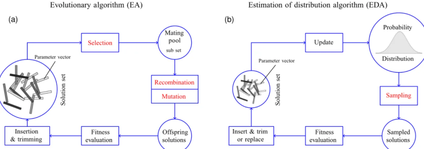
The common goal of such population based meta-heuristics is to strike a good balance of both search prop-erties, exploration (search for promising solutions in a wide area of the search space), and exploitation (search within small regions around good solutions to quickly reach local optima). Classical evolutionary algorithms as depicted on the left of Fig. 1 mimic principles of natural evolution to pursue that goal. They use randomized procedures to select, com-bine, mutate, and reinsert candidate solutions (individuals) from/into a given solution set (population). In each iteration, these mechanisms (red operations in Fig. 1) indirectly imply a probability distribution on the search space with respect to which individuals are likely to appear in the next “genera-tion”. The implied probability distribution changes in each generation, tending to increase the probabilities of good so-lutions and to decrease the probabilities of poor soso-lutions due to the survival-of-the-fittest principle.
In contrast to classical EAs, Estimation of Distribution Al-gorithms (sketched on the right of Fig. 1) use an explicit (pa-rameterized) probability distribution from which candidate solutions are sampled directly. In each iteration, the probabil-ity distribution is also updated directly by utilizing good so-lutions of the current iteration. Good soso-lutions of preceding iterations are (optionally) considered by involving preceding probability distributions into the update process using auxil-iary variables. Evolutionary frameworks use operators (EAs) and probability distributions (EDAs) that are appropriate for the search space under consideration. For example, so-called quantum inspired evolutionary algorithms (QiEA) have been shown to be very suitable EDAs for binary problems (e.g., Kliemann et al., 2013; Patvardhan et al., 2015, 2016). QiEA versions for continuous problems have also been investigated in the literature (Babu et al., 2009).
Evolutionary algorithm (EA)
Solution
set
Parameter vector
Selection
Mating pool sub set
Recombination Mutation
Offspring solutions Fitness
evaluation Insertion
& trimming
Estimation of distribution algorithm (EDA)
Solution
set
Parameter vector
Update
Probability
Distribution
Sampling
Sampled solutions Fitness
evaluation Insert & trim
or replace
(a) (b)
Figure 1.A general EA (left) and EDA (right) schematic. Cycles represent sets of solutions (vectors of BGC parameters in our case) or an explicit probability distribution from which new solutions can be drawn. Rectangle symbols depict operations. Operations displayed in red font depend on random decisions. EA: a set of candidate solutions (population) is iteratively updated. In each generation, candidate solutions compete to form a mating pool which is realized by a random selection operator. Offspring solutions are produced by recombining mates and/or introducing some mutation. Finally, there is a fitness based insertion back into the population, which is usually trimmed to a predefined population size. The random operators selection, recombination, and mutation imply an implicit probability distribution on the search space with respect to which solutions are likely to appear in the next generation. EDA: candidate solutions of the current iteration’s population are used to update an explicit probability distribution such that the likelihood to sample good solutions increases. New candidate solutions are directly sampled from the probability distribution. Usually, the realization of the probability distribution update ensures that information of former solutions fades out slowly, resisting for several iterations. Therefore, the population may be smaller as an EA population and even be replaced with the entire set of new samples, which is the case for the CMA-ES algorithm we use.
a test bed of 24 continuous benchmark functions presented in Hansen et al. (2009a), finding CMA-ES versions to per-form well, particularly on multi-modal test functions. CMA-ES is invariant regarding both order-preserving transforma-tions of the objective function and rotatransforma-tions and translatransforma-tions of the search space. Invariances of a strategy justify general-izations of empirical results, which encouraged us to choose CMA-ES for our application.
We essentially follow the description of the (µ/µw, λ)–
CMA-ES in Hansen (2016). In Sect. 2.2.2, we illustrate how the distribution is sampled and modified. For the sake of completeness, we present the guiding ideas behind the ex-act procedures in Sect. 2.2.3–2.2.6. The algorithm outline can be found in Sect. 2.3. This basic version does not con-sider bound constraints. We therefore use a penalty function based boundary handling (Hansen et al., 2009b) which we will briefly explain in Sect. 2.2.7.
2.2.2 Normal distributions
In CMA-ES the distribution from which candidate solutions (BGC parameter vectors in our application) are sampled is a multi-variate normal distribution. It generalizes the usual normal distribution, also known as Gaussian distribution, from Rto the vector spaceRn with arbitrary dimensionn, given by the number of biogeochemical parameters to be es-timated. The position and the shape of the one-dimensional
normal distribution (more precisely, its density function) is uniquely defined by its mean and its variance, respectively.
A measure of the “diversity” of a probability distribution is the so-called (differential) entropy. For a given variance, the normal distribution has the maximum entropy amongst all distributions with the same variance (Cover and Thomas, 2006; Hansen, 2016). Entropy is used as an index of diversity, though it does not directly mean the same as diversity (Jost, 2006).
-0.5 0 0.5 0 1 2 3 Iteration 1
-0.5 0 0.5
0 1 2 3
Iteration 16
-1 0 1 -1
0
1 Iteration 1
-1 0 1 -1
0
1 Iteration 4
-0.5 0 0.5
0 1 2 3
Iteration 2
-0.5 0 0.5
0 1 2 3
Iteration 22
-1 0 1 -1
0
1 Iteration 2
-1 0 1 -1
0
1 Iteration 5
-0.5 0 0.5
0 1 2 3
Iteration 3
-0.5 0 0.5
0 1 2 3
Iteration 28
-1 0 1 -1
0
1 Iteration 3
-1 0 1 -1
0
1 Iteration 6
(a) (b)
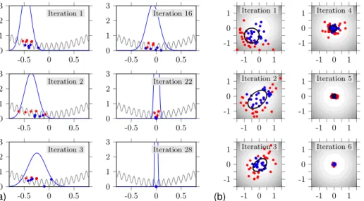
Figure 2.Iterations of the CMA-ES applied to test functions. Left: a uni-variate Griewank-type functionf(grey curve). In each iteration we drawλ=10 samples from the normal distribution (blue curve). For each samplexi, the pair(xi, f (xi))is marked with a dot. Theµ=λ2=5 better samples (blue dots) are involved in the normal distribution update for the next iteration. Right: two-dimensional sphere function. Here, samples are marked with dots, while function values are indicated by the grey levels in the counter plots; theith grey level represents the rangehi−21,2i. More samples (50) than necessary are used to update the distribution, which is indicated by its standard deviation ellipse (black), here. Distributions tend to elongate into directions of descent (iteration 2). For the convex example function, the algorithm converges after a few iterations.
attracted towards the good samples, then. Also, the distribu-tion shape widens, after good samples had some distance to each other and/or some distance to the current mean. Vice versa, if all good samples are close to the mean, the shape will narrow, again. Now, the mean of the distribution is sup-posed to drift towards the global optimum and should then start to narrow more and more. This behavior is observed in iterations 16, 22, and 28. So, when necessary, the procedure is supposed to become less exploring but more exploiting.
Similarly to the definition of the uni-variate Gaussian tribution by mean and variance, a multi-variate normal dis-tribution can be uniquely identified by a mean vectorxand a positive definite matrixCof covariances, respectively, and is denoted by N(x,C). Again, the mean defines the center of the distribution, while the covariance matrix defines its shape. The area of 1 standard deviation which is an inter-val[x−σ, x+σ]in the one-dimensional case becomes ann -dimensional ellipsoid, now (cf. the ellipses on the right side of Fig. 2 forn=2). It can be shown that the principal axes of the ellipsoid correspond toC’s eigenvalues and eigenvectors, respectively. More precisely, an eigenvector defines the ori-entation of a principal axis and the square root of the corre-sponding eigenvalue defines the length of that principal axis. 2.2.3 Sampling the distribution
Sampling a multi-variate normal distributionN(x,C)can be practically implemented using an eigendecomposition C= BD2BT, whereD2is a diagonal matrix of eigenvalues ofC and Bis a matrix of corresponding orthonormal
eigenvec-tors ofC. One samplex∈RnofN(x,C)can be realized by drawingnindependent random numbers from the uni-variate standard normal distributionN(0,1)to be the components of a random vectorz∈Rnand settingx=x+BDz.
Note that for our problem there are bound constraints on the parameters such that samples of a normal distribution might be infeasible, regardless of whether the distribution mean is feasible or not. However, a boundary handling proce-dure (see Sect. 2.2.7) will ensure that the optimization result of CMA-ES is feasible.
2.2.4 Updating the distribution: basic principle
Empirical (re)estimatesxempandCempof the distribution
pa-rameters can be calculated from a setS= {x1, . . .,xλ}ofλ
samples, such that the expectation ofxempisx and the
ex-pectation ofCempisC:
xemp=
1 λ
λ X
i=1 xi,
Cemp=
1 λ−1
λ X
i=1
(xi−xemp)(xi−xemp)T.
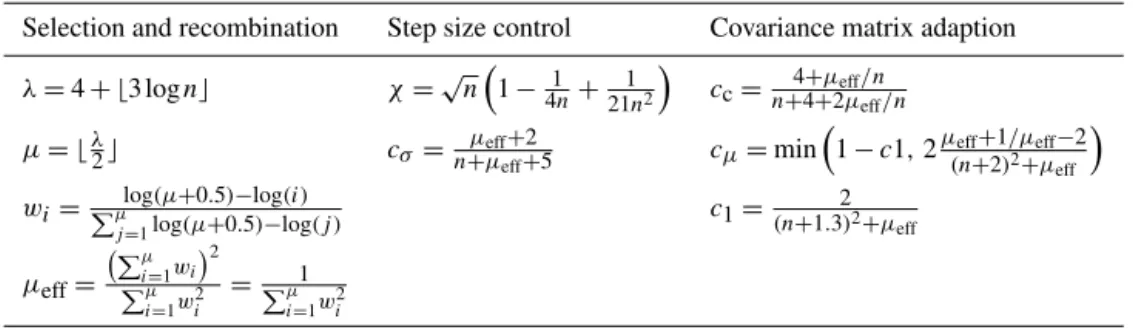
Table 1.Operational constants of the CMA-ES algorithm (cf. the initialization in Algorithm 1).
Selection and recombination Step size control Covariance matrix adaption
λ=4+ ⌊3 logn⌋ χ=√n
1−4n1 + 1 21n2
cc= 4+µeff/n
n+4+2µeff/n
µ= ⌊λ2⌋ cσ= µeff+2
n+µeff+5 cµ=min
1−c1,2µeff+1/µeff−2
(n+2)2+µ eff
wi= Pµlog(µ+0.5)−log(i) j=1log(µ+0.5)−log(j )
c1= (n 2 +1.3)2+µ
eff
µeff=
Pµ
i=1wi 2
Pµ
i=1w2i = 1
Pµ
i=1w2i
function f :Rn−→R, that is, f (x1)≤f (x2). . .≤f (xλ).
Now, by involving only the better half of µ= ⌊λ2⌋ sam-ples, their distribution estimateN(xµ,Cµ)with correspond-ing parametersxµandCµwill be biased towards
reproduc-ing µ samples with higher probability than the otherλ–µ samples. CMA-ES uses positive valuesw1≥w2≥. . .≥wµ
withPn
i=1wi=1 to give solutions a rank dependent weight
in the updating process of both,xµandCµ. The exact
CMA-ES formula for thewvalues and information about its back-ground is found in Sect. 2.3.1. The new mean is, thus, cal-culated asxµ=Pµi=1wixi. A subtlety is the choice of the
reference mean value used for estimatingCµ. Instead of the
new empirical meanxµ, the meanx of the former
distribu-tion is chosen and yields Cµ=
µ X
i=1
wi(xi−x)(xi−x)T. (1)
It has the effect that the new distribution is elongated into directions of descent (see iteration 2 in the right example of Fig. 2).
2.2.5 Updating the distribution: reliability with small populations
As mentioned above, reliable distribution estimates require a sufficiently large number of samples. However, for a com-petitive computational performance we must get along with a rather small number of samples. CMA-ES therefore involves the information of former populations by updating the co-variance matrixCto be a (convex) combination of both the currentCand its estimateCµ, that is,
C ← (1−cµ)C+cµCµ. (2)
Using this formula, it can be shown that 37 % of the current matrixC’s information dates back at least⌊c1µ⌋generations;
that is, the choice of the smoothing factor cµ decides the
backward time horizon of the update procedure. The smaller the factorcµin Eq. (2) is, the more former samples contribute
to the current distribution estimate, slowing down learning but being more reliable, with fewer samples per iteration. For example, the experiments in this paper usen=6 param-eters and λ=10 samples per generation. Using Eq. (2) to
updateCand the (compromise)cµvalue defined for
CMA-ES (see Table 1), the samples of the last 23 iterations would contribute roughly 63 % of the overall information inC.
Another feature that facilitates small population sizesλis to calculate and update a vectorpcthat represents
iteration-averaged changes of the distribution mean and to usepcfor
a so-called rank-one estimateC1=pcpTc of the covariance
matrix. The idea behind this approach is that, usingCµ,
tribution elongations into directions of descent do not dis-tinguish for the sign of the directions. The use of the vector pc(called the evolution path) mitigates this effect. Consecu-tive changes of the distribution mean into opposite directions would cancel out each other. Similar to the smoothing with factorcµin the update ofC, above, the update ofpcis done
with a smoothing factor cc. With a further smoothing
fac-torc1for the rank-one estimateC1, the combined covariance
matrix update reads
C ← (1−cµ−c1)C+cµCµ+c1C1.
WhileCµefficiently involves information from the current
population in the update process,C1exploits correlations
be-tween generations. The former is important in large popula-tions; the latter is particularly important in small populations. 2.2.6 Step size control
Finally, there is an additional explicit adaption of the overall scale (the step size) of the distribution by adapting a scal-ing factorσ, actually usingN(x, σ2C)instead ofN(x,C).
Similar to the evolution path pc for the rank-one
covari-ance matrix estimates above, the adaption of the scaleσ in-volves an evolution pathpσ that mirrors cumulative changes in the mean. The difference between the update formulas of both evolution pathspσ andpc is that forpσ each change is re-scaled (normalized) with respect to the isotropic nor-mal distribution N(0,I). Since covariances are always re-estimated with respect to the mean of the former iteration (cf. Eq. 1), the expected normalized change of the distribu-tion mean per iteradistribu-tion is therefore the expected length of a sample ofN(0,I), which is
χ:=E(kN(0,I)k)≈√n
1− 1 4n+
1 21n2
Now, a rather small lengthkpσ kcompared toχ indicates that consecutive normalized moves of the mean canceled each other out, meaning that the overall scale of the dis-tribution should be reduced with σ. Vice versa, an evolu-tion pathpσlonger thanχindicates consecutive distribution drifts into correlated directions, which justifies a larger over-all scale of the distribution.
2.2.7 Boundary handling
In order to consider boundary constraints, we use the pro-cedure proposed in Hansen et al. (2009b, Sect. IV B) for CMA-ES. It applies if the distribution mean runs out of bounds. In this case, the fitness of an unfeasible sample x becomes the sum of the fitness of its closest feasible point xfeas and a weighted quadratic penalty function of its
dis-tancekx−xfeaskto the feasible box (toxfeas). Feasible
sam-ples are not penalized; i.e., the penalty function is 0 within the feasible box. Thus, the minimum of the sum of the actual fitness function and the penalty function is taken inside the feasible box or on its boundary. The quadratic penalty func-tion has coordinate-wise weights γi
ξi, whereξiscales the
out-of-bounds distance in the ith coordinate with regard to the shape of the current distribution. Theγi are suitably
initial-ized with the range of former (unpenalinitial-ized) objective func-tion values and is multiplied by a constant>1 in every iter-ation in whichxi is more than 3 standard deviations off its
bounds.
In our implementation of CMA-ES, the feasible box we operate on is the unit cube [0,1]n⊆Rn. The samples are then linearly transformed (encoded) with respect to the ac-tual bound constraints before evaluating the objective (misfit) function.
2.3 Implementation of the optimization algorithm
2.3.1 Algorithm outline
The CMA-ES approach described in Sect. 2.2 allows for reli-able covariance matrix estimates with a relatively small pop-ulation size. The default poppop-ulation size ofλ=4+3 log(n) individuals and all further operational constants are succes-sively derived from the problem dimensionnas outlined in Table 1.
Here,µcounts the good portion of individuals that are se-lected from theλsamples in each iteration and used to up-date the probability distribution. As mentioned in Sect. 2.2.4, sampled individuals are always sorted with respect to their function values (f (x1)≤. . .≤f (xλ)).
The µ recombination weights wi sum up to 1 and are
monotonically decreasing in order to give better selected samples a higher weight in the updating formulas. Hansen (2016) suggests using the valueµeffas a quality measure for
the weights and states that µeff=
λ
4 (3)
indicates a good choice. Indeed, Eq. (3) is approximately sat-isfied by the given weighting scheme. We can only briefly sketch the history behind the suggestion: with equal weights
1
µ in the distribution update, all the bestµindependent
sam-ples would count with the same influence. For this case it has been shown with an exemplary uni-modal function (the infinite-dimensional sphere function) that the setting µ= 0.27·λis optimal in the sense that the “expected progress per sample” towards the global optimum is maximized (Hansen et al., 2015, Sect. 4.2.2) (cf. Beyer, 2001, Chap. 3.1.1 and 3.2.1.2). Hansen considers the value µeff to be a
general-ization of the number of selected independent samples that influence the distribution, consequently using the similar Eq. (3) for the case of rank dependent weights. Note thatµeff
takes its maximumµ with equal weights and its minimum 1 if all but one weight are zero. Actually, theoretically opti-mal non-equal weights and, thus, the optiopti-mal value forµeff,
are also known for the infinite-dimensional sphere function (Arnold, 2006, Sect. 3.2). These include non-zero weights for allλsamples and negative weights for the worse λ2 sam-ples (hence doubling the value ofµeff). However, negative
weights are not considered to be a robust enough practical choice.
Together with the problem dimensionn, the generalized number of independent selected samples µeff appears in
the calculation of the four smoothing constantscσ, cc, cµ, c1
used in the update formulas of both the evolution paths and the covariance matrix. Their dependence onnandµeff has
been derived empirically. The constantχ (cf. Sect. 2.2.6) is approximately the expected norm of then-dimensional stan-dard normal distributionN(0,I).
The algorithm details are summarized in Algorithm 1. It starts with the identity matrixIfor the covariances, that is, with an isotropic distribution. Assuming the optimum so-lution to reside within the unit cube[0,1]n⊆Rn, the mean xand the overall scaleσare initialized according to Hansen (2016). Actually, having bound constraints (cf. Sect. 2.2.7), we operate on the unit cube and shift and scale obtained samples into their real bounds before calculating their objec-tive function values. New samples are drawn as described in Sect. 2.2.3. Theykcorrespond to thexk−xconsidered there,
divided by the step sizeσ. The newx is calculated accord-ing toxµin Sect. 2.2.4. Note thatyis theσ-adjusted move of
in Sect. 2.2.6 and 2.2.5, respectively. For the given weights w the factor cσ
1+cσ in the update formula of σ is equal to a
more general formulation used, e.g., in the CMA-ES tutorial (Hansen, 2016). We stop either after the predefined number of iterations or if the current population shows a flat misfit distribution, i.e., if the fitness of the better 70 % of the indi-viduals deviates less thanǫ=10−5from the very best one.
Algorithm 1The(µ/µw, λ)-CMA-ES
Initialization:
Setλ, µ, w, µeff, χ , cσ, cc, cµ, c1according to Table 1
Setx=(12, . . . ,12)T
Setpσ=pc=0, C=B=D=Iandσ=0.5
whilestopping criterion∗)is not metdo Sample probability distribution:
fork=1, . . . , λdo
Samplezk∈RnfromN(0,I)by sampling its entries fromN(0,1)
Setyk=BDzkandxk=x+σyk end for
Update probability distribution: Update mean:
x ← Pµ
k=1wkxk
Sety=Pµ
k=1wkykandy∗=BD−1BTy
Update evolution paths:
pσ ← (1−cσ)pσ+pcσ(2−cσ)µeffy∗
pc ← (1−cc)pc+pcc(2−cc)µeffy
Update covariances and scaling: σ ← σ·exp cσ
1+cσ
kpσk
χ −1
SetCµ=Pµk=1wkykyTk andC1=pcpTc
C ← (1−cµ−c1)C+c1C1+cµCµ
DetermineBandDfrom eigendecomposition C=BD2BT
end while
∗) our stopping criterion is that either a predefined number of
iterations is reached or the fitness distribution is flat (see text)
2.3.2 Algorithm parallelization
Our current technical implementation of the parallel frame-work can be easily transferred to other EAs/EDAs. The iter-ative optimization process is carried out via a series of chain jobs, where short serial jobs (the actual optimizer) that up-date the population of model evaluations (“individuals”; i.e., parameter sets for biogeochemistry) alternate with parallel jobs of function evaluations (“generations”), i.e., forward in-tegrations of the coupled ocean model with different param-eter sets. Paramparam-eters of the optimizer are population size λ and the termination criterion for convergence; additionally, a maximum number of iterations.
As noted above, the framework presented here is set up such that a serial scriptserial.jobcalls the optimization routine (in our case CMA-ES), which computes a popula-tion of size=λof parameter vectors, stored in ASCII files. The same script then calls a parallel scriptparallel.job, which startsλmodel simulations. During these simulations,
the parameter files are read, and a spinup is carried out for each individual setup. The individual model runs then output the misfit function to specified files. When all jobs are fin-ished, scriptparallel.jobinvokes scriptserial.job
again, etc. Thus, communication between both alternating steps (creation of parameter vectors and computation of the resulting misfit function) is carried out by these parameter and misfit files. In addition, filenIter.txtkeeps track of the progress of optimization, and provides the information on which generation is to be computed; it also contains the run-time parameters for the optimizer, CMA-ES. See the infor-mation in the Supplement for more details on how this setup works, and how to specify the biogeochemical and optimizer parameters used, e.g., in the work presented here.
2.4 Misfit function
As a first approach to optimization, we have calculated the root-mean-square error RMSE between simulated and ob-served (or twin) annual mean phosphate, nitrate, and oxygen concentrations on a global scale, weighted by the volumeVi
of each individual grid box, expressed as a fraction of total ocean volume,VT. To sum the three different components of
the misfit function, we have to divide them by some typi-cal value. Here we use the global mean concentration of ob-served tracers. The resulting misfit functionJthus reads as
J= 3 X
j=1
1 oj v u u t N X
i=1
(mi,j−oi,j)2 Vi VT
(4)
for the annual mean concentrations of three tracers phosphate (j=1), nitrate (j =2), and oxygen (j=3), atN=52 749 locations (model grid boxes) of the model domain.oj is the
global average observed (or twin) concentration of the re-spective tracer.mi,j andoi,j are model and observations (or
twin results), respectively. By weighting the model mismatch with volume, we put some emphasis on the deep ocean, down-weighting deviations in surface grid boxes relative to those of deep boxes. Thus, our misfit function serves more as a long timescale geochemical estimator, in contrast to a function that focuses on (rather fast) turnover in the surface layer.
2.5 Parameters to be estimated
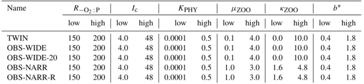
si-Table 2.Experimental setup of optimization. “low” and “high” indicate boundary constraints of the optimizations, respectively.
Name R−O2:P Ic KPHY µZOO κZOO b∗
low high low high low high low high low high low high
TWIN 150 200 4.0 48 0.0001 0.5 0.1 4.0 0.0 10.0 0.4 1.8 OBS-WIDE 150 200 4.0 48 0.0001 0.5 0.1 4.0 0.0 10.0 0.4 1.8 OBS-WIDE-20 150 200 4.0 48 0.0001 0.5 0.1 4.0 0.0 10.0 0.4 1.8 OBS-NARR 150 200 4.0 48 0.0001 0.5 1.0 3.0 1.6 4.8 0.4 1.8 OBS-NARR-R 150 200 4.0 48 0.0001 0.5 1.0 3.0 1.6 4.8 0.4 1.8
∗Note that fromb(the optimized parameter) in the model we calculate the rate of vertical increase in sinking speeda, always assuming a nominal detrital remineralization ofr=0.05d−1. The resulting values foraare 0.058275 (target (twin)), 0.125 (high), and 0.027778 (low).
multaneous optimization of parameters that are obviously re-lated to each other, such as maximum growth rates and half-saturation constants, or sinking speed and remineralization rate.
Four parameters are more relevant for biological interac-tions at the sea surface. Phytoplankton growth is controlled by the half-saturation for light (Ic, in W m−2) and phosphate
(KPHY, in mmol P m−3). For optimization of zooplankton
pa-rameters we chose its maximum grazing rate (µZOO, in d−1)
and quadratic mortality rate (κZOO, in (mmol P m−3)−1d−1).
Two parameters are of importance for the transport and decay of particulate organic matter to/in the deep ocean, namely the ratio of oxygen consumption to phosphate release during aer-obic remineralization (R−O2:P, mmol O2: mmol P) and the parameter for vertical increase in sinking speed of organic matter, a (d−1). Note that, as stated above, in the follow-ing, and during optimization, we express this last parameter throughb=r/a, withrheld constant atr=0.05 d−1.
For each parameter we initially chose a rather wide range of possible parameter values (Table 2). The lower value of R−O2:Pwas set to 150 mmol O2: mmol P (Anderson, 1995), while its upper value is at the upper end of observed values (Boulahdid and Minster, 1989), and closer to values used in previous model studies (Paulmier et al., 2009).b is allowed to vary between low values observed mainly in oxygen min-imum zones (Van Mooy et al., 2002), and twice the global open ocean composite derived by Martin et al. (1987); its range is slightly larger than the range applied in previous modeling studies (Kwon and Primeau, 2006; Kriest and Os-chlies, 2008; Kriest et al., 2012), or the range ofbdetermined from in situ observations (e.g., Martin et al., 1987; Buesseler et al., 2007). It agrees with the range ofbderived from indi-rect estimates ofb(Henson et al., 2012; Marsay et al., 2015). Ranges of parameters related to surface processes were more difficult to assign. Due to the highly aggregated form of the organic biological components in the model, these pa-rameters are supposed to reflect a variety of processes such as species shift and adaptation (e.g., half-saturation constants for nitrate uptake may vary over several orders of magnitude; see Collos et al., 2005). We therefore initially assigned very wide boundaries forIc,KPHY,µZOO, andκZOO, which allow
the optimization to pick parameters that virtually may shut down certain biological fluxes and processes. The choice of these wide boundaries, its consequences for optimization and model performance, and the effects of narrower boundaries will be examined and discussed below.
2.6 Setup and performance of optimization
Using the combined framework described above, i.e., TMM+MOPS+CMA-ES, we carried out five different full optimizations, with the aim of determining the four param-eters related to surface biology and two paramparam-eters more closely tied to the deep biogeochemistry mentioned above. The experiments differ with respect to the observations used for the misfit function (model output, climatologies of obser-vations), population sizeλof CMA-ES (10 or 20 individu-als per generation), parameter boundaries, and the sampling strategy of CMA-ES. They are explained in detail below. 2.6.1 TWIN experiment
First we tested the ability of CMA-ES to recover known pa-rameters of a model simulation that applied the same biogeo-chemical parameters as MOPS-RemHigh of Kriest and Os-chlies (2015, setup “base”, i.e., with a particle flux described byb=0.858, ora=0.058275, and a high affinity of oxic and suboxic remineralization to oxidants). This is done by optimization against its simulated annual average phosphate, nitrate, and oxygen of year 3000. We refer to this experiment as “TWIN”. TWIN applies rather wide boundaries for all pa-rameters (see Table 2), and a population size for CMA-ES ofλ=10, which was deemed sufficient for six parameters, given the default configuration of the CMA-ES (see above). 2.6.2 Optimizations against observed tracers
it-Table 3.Optimization results (evaluations, i.e., number of individuals,λ, times number of generations,N), best model misfitMopt, optimum parameters, and their uncertainties. For each model and parameter, the first line gives the optimum parameter, followed bypminand maximum pmaxof all individuals, for which the misfitMiis(Mi−Mopt)/Mopt≤0.001. The third line additionally presents in parentheses the percent of individuals for which this criterion holds, as well as the range of optimum parameters as a percent of the average parameter of the last generation. We also give the misfit and parameters of the reference run, against which the twin experiment was optimized.
Experiment λ×N Mopt R−O2:P Ic KPHY µZOO κZOO b
Reference 1 0.529 170.0 24.0 0.03125 2.0 3.2 0.858
TWIN 2000 0.0003 170.0 24.0 0.034 2.0 3.20 0.858
170 24 0.033–0.035 2.0 3.19–3.20 0.858 (<1) (<1) (<1) (5) (<1) (<1) (<1)
OBS-WIDE 950 0.477 179.5 48.0 0.12 0.28 6.15 1.10
176–182 46–49 0.09–0.13 0.24–0.32 4.79–3.37 1.08–1.12
(31) (3) (6) (32) (28) (26) (4)
OBS-WIDE-20 3460 0.450 167.7 9.9 0.5 2.05 5.83 1.34
165–171 9.6–10.8 0.39–0.57 2.00–2.52 5.37–10.0 1.31–1.37
(64) (3) (12) (34) (25) (79) (5)
OBS-NARR 1820 0.450 167.0 9.7 0.5 1.89 4.57 1.34
165–170 9.0–10.3 0.39–0.53 1.57–2.02 2.95–4.66 1.30–1.36
(39) (3) (14) (28) (23) (37) (4)
OBS-NARR-R 1400 0.450 166.7 9.6 0.5 1.76 3.82 1.34
165–169 8.7–10.1 0.44–0.54 1.57–1.79 2.77–3.90 1.31–1.36
(50) (2) (14) (19) (13) (30) (3)
self, the experiments differ in the upper and lower boundaries of the search space for zooplankton parameters, the popula-tion size λ of CMA-ES, and its sampling strategy. This is done in a stepwise fashion.
Experiment OBS-WIDE differs from TWIN only with re-spect to the observations that enter the misfit function. In OBS-WIDE we encountered an unlikely (with respect to bi-ological tracer concentrations) solution, pointing towards a potential local minimum in the misfit function. We therefore set up two experiments to investigate strategies to improve the performance of CMA-ES with respect to more plausible solutions. The experiments both increase the search density in the parameter space with respect to OBS-WIDE. In experi-ment OBS-WIDE-20 search density is increased by doubling the population size of CMA-ES to λ=20. Otherwise, its setup is the same as OBS-WIDE. In experiment OBS-NARR we keepλ=10 of OBS-WIDE, but restrict the boundaries for zooplankton parameters to±50 % of the value of the ref-erence run of MOPS.
Because optimization OBS-NARR showed the best results with respect to misfit function, biogeochemical fluxes, and optimization performance (see below; Tables 3 and 4), in ex-periment “OBS-NARR-R” we finally evaluate the robustness of optimization OBS-NARR by repeating this optimization with a different random selection of the parameter values from the distribution calculated by CMA-ES.
2.6.3 Performance
The internal termination criterion of CMA-ES was reached after 95, 173, 182, and 140 generations for OBS-WIDE, OBS-WIDE-20, OBS-NARR, and OBS-NARR-R, respec-tively. For the twin experiment, we restricted the maxi-mum number of generations to 200, at which TWIN had approached the target parameters, the misfit declined to <0.0004 (i.e., on average less that 0.2 ‰ of global mean tracer concentrations; see Eq. 4) and fitness variance declined to <10−9. As presented above, in each “generation” we computed 10 (20) different “individuals” (model simulations over 3000 years) in parallel. One simulation of each genera-tion on average took≈1.25 h, on 40 (80) nodes of Intel Xeon IvyBridge or Intel Xeon Haswell at the North-German Su-percomputing Alliance (HLRN). We note that tests on either hardware (two iterations of the coupled code, started from generations 80 and 160 of experiment TWIN) did not re-veal any differences in the estimated fitness. The CMA-ES – which, due to its very short runtime, is not parallelized – was always computed on one core of Intel Xeon IvyBridge.
3 Results
3.1 Twin experiment (TWIN)
Table 4.Global annual fluxes of primary production (PP), grazing (GRAZ), aerobic and anaerobic remineralization of detritus and DOM to nutrients (REM), excretion by zooplankton (EXCR) export production (F120, flux through 120 m), flux through 2030 m (F2030), and benthic burial (BUR), in Pg N year−1, for the reference experiment, OBS-WIDE, OBS-WIDE-20, and OBS-NARR (two repeated experiments with different configurations of CMA-ES). We also show some globally derived, observed estimates. Conversion between different elements was carried out via N : P=16 and C : P=122.
Experiment PP GRAZ REM EXCR F120 F2030 BUR
Reference 5.44 3.52 4.72 0.80 0.92 0.11 0.05 OBS-WIDE 6.20 1.24 5.94 0.25 0.81 0.06 0.02 OBS-WIDE-20 7.45 4.68 6.66 1.00 1.10 0.06 0.02 OBS-NARR 7.52 4.74 6.65 1.10 1.10 0.06 0.02 OBS-NARR-R 7.58 4.77 6.65 1.19 1.10 0.06 0.02 Observed∗ 7.68–8.09 4.79, 5.71 – – 0.29–1.53 0.03–0.07 0.02
∗Observed fluxes are from Carr et al. (2006, primary production), Honjo et al. (2008, particle flux), Lutz et al. (2007, particle flux), Dunne et al. (2007, particle flux), Schmoker et al. (2013, primary production, zooplankton grazing excluding/including mesozooplankton grazing) and Wallmann (2010, burial; without shelf and slope region).
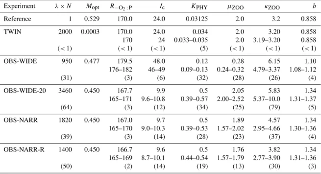
Figure 3.Optimization trajectory for six parameters of the twin experiment. The thick black line shows the average parameter of all 10 individuals of a generation. Red lines indicate their maximum and minimum parameter values. Horizontal black lines indicate the target parameter. Note that we restrict they-axis to the maximum and minimum boundaries.
exceeding the prescribed boundaries. This results in high maximum and minimum misfits (Fig. 4), and this high vari-ability is maintained over about 10–20 generations. The tra-jectory of transient average parameter values and their vari-ance depend strongly on the parameter itself: while the two parameters associated with rather long timescales, namely the stoichiometric ratio R−O2:P and exponent b describ-ing particle sinkdescrib-ing, approach their target values quite early (about generation 20–40), parameters associated with sur-face biogeochemistry stay far away from their target value for ≈80 generations (Ic, KPHY,κZOO) or oscillate around
it (µZOO). After ≈160 generations, most of the
parame-ters reached their target value, the exception being the half-saturation constant of phytoplankton for phosphate uptake, KPHY(Table 3). This parameter still shows considerable
vari-ability at the end of the optimization (generation 200), al-though by that time is it quite close to the – rather low – target value.
m v
(a) (b) (c)
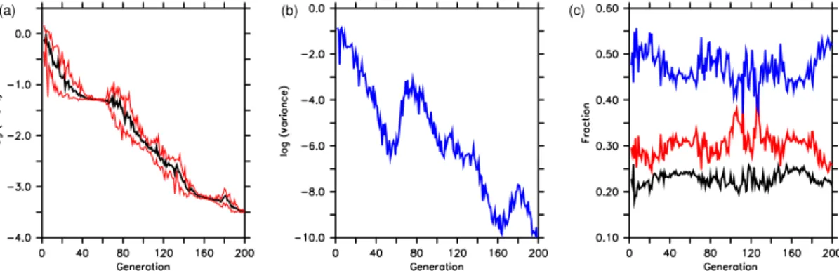
Figure 4.Model misfit, its variance, calculated from individuals of each population (both transformed logarithmically by log10) and compo-nents of the twin experiment. Left panel: the thick black line shows the average misfit of all 10 individuals of a generation. Red lines indicate the maximum and minimum misfit. Mid panel: variance of misfit. Right panel: contribution of each component of the misfit function. Blue: oxygen. Red: nitrate. Black: phosphate.
Figure 6.As Fig. 5, but only plotted for a region±2 % around the average parameter value of the last generation, regardless of generation and associated misfit. Note that these parameters can have occurred early in the optimization and even be associated with a large misfit (that would arise from at least one of the other parameters, causing a large misfit). Note that the color scale is different than in Fig. 5.
Further increases in variance can be seen around generation 100, and, at the end, when the algorithm widens its search area again, probably in search of an optimalKPHY. It seems
encouraging that the algorithm does not get stuck in a local minimum, but, at the expense of deterioration of the misfit, continues to search for an even better parameter set.
The largest fraction of the misfit function is related to oxy-gen, followed by the misfit to nitrate, and then phosphate. The dominance of oxygen and nitrate is not surprising, as these tracers are not conservative; i.e., their global inventory might change due to air–sea gas exchange, denitrification, and nitrogen fixation (see also Kriest and Oschlies, 2015), so that the model may not only err with respect to the spa-tial distribution of these tracers, but also with respect to their global mean concentration.
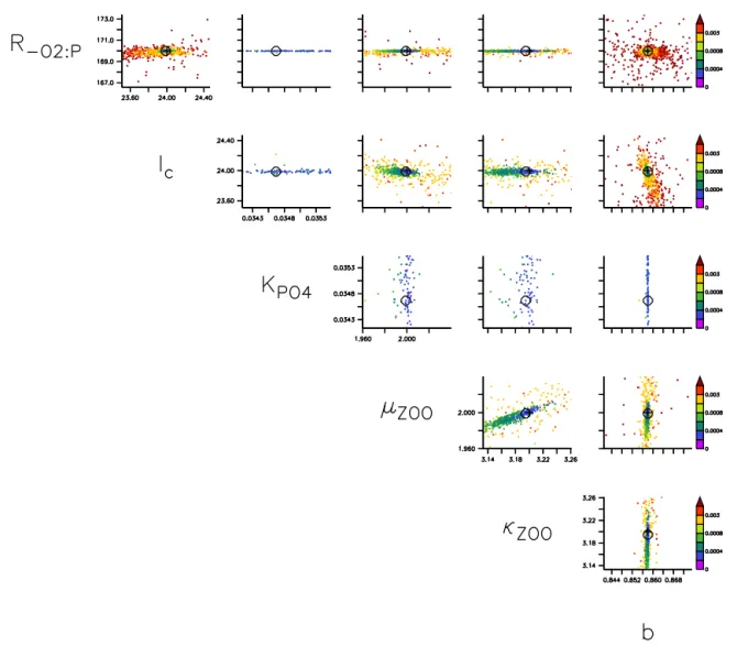
In Fig. 5 we finally exploit the shape of the misfit function, shown on a color scale for every two pairs of parameters. As can be seen from the misfit plotted againstR−O2:Pandb
(upper right corner), these two parameters are quite well con-strained, with a very well-defined minimum around the tar-get value. All other parameters show more or less elongated search “canyons”. Much of the algorithm search starts away from the target value; however, the algorithm finally manages to approach the target value even when the search path is not straight, but curved in the two-dimensional projections of the parameter space. Further, even when the algorithm exceeds the target value (e.g., for the maximum growth rate of zoo-plankton,µZOO; lower right corner), despite the already low
misfit function, the algorithm finally returns to the somewhat lower value (compare also to Fig. 3, lower left panel).
pa-v
(a) (b) (c)
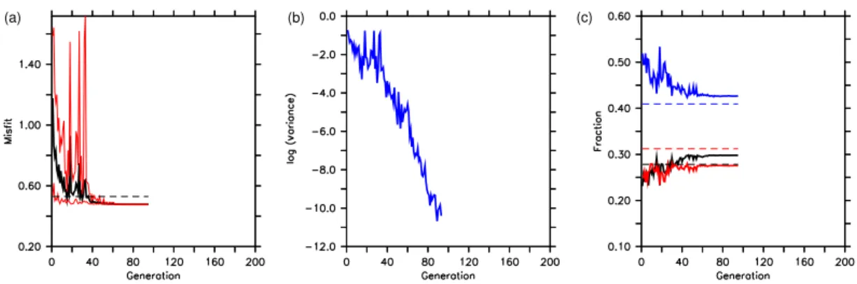
Figure 7.As Fig. 4, but for optimization OBS-WIDE. Note that in the left plot, we now show the raw value of the misfit function (not log transformed). The optimization finished at generation 95.
rameter the search landscape becomes quite uninformative (Fig. 6), with similar misfits around ±2 % of its last value. Thus, a low misfit can be achieved within a wide range of this parameter.
One reason for this low sensitivity of the misfit function toKPHYmay be found in the fact that, in the twin, against
which the model is optimized, only very few (1 %) phos-phate values are at or below the target value of KPHY=
0.03125 mmol P m−3. Therefore, besides the dominance of oxygen in the misfit function (Fig. 4), the misfit function is further dominated by phosphate concentrations outside the oligotrophic surface regions, rendering it quite insensitive to changes in the half-saturation constant at low values. In addi-tion, a closer look at the misfit topography (Fig. 5) points to-wards a potential correlation ofµZOOandκZOO, which may
complicate the algorithm’s search for an optimum set of pa-rameters, thereby slowing down its convergence.
3.2 Optimization against observed nutrients and oxygen distributions
3.2.1 Wide boundary constraints for zooplankton (OBS-WIDE, OBS-WIDE-20)
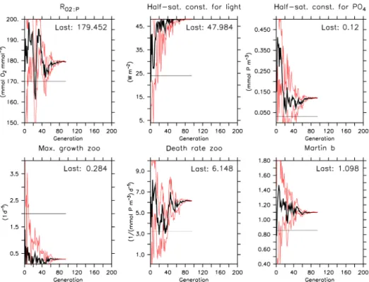
When optimizing the model against observed concentrations with exactly the same setup as for experiment TWIN, opti-mization OBS-WIDE reaches the internal termination crite-rion of the CMA-ES at generation 95. Instead of declining exponentially towards zero, the misfit only declines from an average initial value of≈0.8 to 0.477 (Fig. 7, Table 3), i.e., only slightly less than the misfit of the reference run (0.529). Also, the variance of misfit as well as that of the parameters show a more or less gradual decline, without any intermittent increase (see the Supplement). Another notable difference to TWIN is the higher contribution of phosphate to the misfit function (Fig. 7).
Some parameters diverge strongly from those of the ref-erence run. In particular, the phytoplankton’s half-saturation constant for light, Ic, increases strongly up to its upper
boundary (Fig. 8; Table 3; see also the Supplement for a
plot of the topography of the misfit function). However, the stronger light limitation of phytoplankton growth is coun-teracted by a strong decrease in zooplankton growth rate, µZOO, and a strong increase in its quadratic mortality rate, κZOO. As a consequence, average and maximum
zooplank-ton concentrations are<25 and<50 % of that of the ref-erence run in the surface layer (Fig. 9), while phytoplank-ton is strongly increased, when compared to the reference run. Most likely because the zooplankton–detritus pathway is nearly shut off, DOM concentrations are strongly increased. The reorganization of the pelagic food web in this optimized model scenario is reflected in the global annual biogeochem-ical fluxes: primary production is enhanced by almost 14 %, but loss through grazing is reduced to about 1/3 of that of the reference run (Table 4). As a consequence, the largest frac-tion of recycling is through remineralizafrac-tion of detritus and DOM (>95 % of annual production), and only 4 % through zooplankton excretion, while in the reference run zooplank-ton recycles almost 15 % of annual production. Due to the reduced particle sinking speed, shallow (130 m) and deep (2030 m) particle fluxes are reduced, as is benthic burial. While some of the simulated fluxes are within the observed estimates, overly low zooplankton concentration, as well as the resulting low zooplankton grazing, are far outside ob-served estimates (see Table 4).
Therefore, although optimization OBS-WIDE against ob-servations has decreased the misfit to obob-servations to≈90 % of that of the (subjectively tuned) reference run, the outcome is not overly satisfying with respect to the optimized param-eters and the resulting dynamical behavior of the model. Ob-viously, the very wide boundary constraints we chose for the zooplankton parameters led to a solution where zooplankton is almost dead – a statistically optimal but biologically mean-ingless solution.
Figure 8.As Fig. 3, but for optimization OBS-WIDE. The optimization finished at generation 95.
over a longer period, again, as for optimization TWIN, with intermittent increases in variance during the course of the op-timization. Most importantly, using the setup of OBS-WIDE-20, the optimization finds very different parameters for many of the biogeochemical components.
R−O2:P is now closer to the a priori value of 170, while optimalbhas increased considerably tob=1.34 (Table 3). The largest difference to both the reference run as well as optimization OBS-WIDE occurs for the four biogeochemical parameters that are more closely tied to surface processes:Ic
decreases to less than 50 % of its a priori value, whileKPHY
is at its upper boundary of 0.5 mmol P m−3. Encouragingly, zooplankton parameters are now such that zooplankton is vi-able (Fig. 9). Its maximum growth rate is very close to the a priori value of 2 d−1. Its mortality rate is still quite high; however, because of its high growth rate, zooplankton plays a considerable role in the pelagic nitrogen budget, with global fluxes much closer to the observed ones than for optimization OBS-WIDE (Table 4). The topography of the – rather dense – scan of the parameter space of OBS-WIDE-20 (Fig. 12) points towards a potential correlation betweenKPHY,µZOO,
andκZOO. In this projection, low misfit values occur along
a concomitant increase in KPHYwith eitherµZOO orκZOO.
This is also reflected in the high level of parametric uncer-tainty, as revealed by a large range of parameter values in the vicinity of the optimum (Table 3).
Summarizing, using a larger population size and thus a denser scan of the parameter space (see Fig. 12), CMA-ES has found a better solution with respect to the misfit function
(see Table 3) as well as a closer fit to biogeochemical fluxes and more plausible biological patterns.
3.2.2 Narrow boundary constraints for zooplankton (OBS-NARR and OBS-NARR-R)
Optimizations with a population size ofλ=20, as for OBS-WIDE-20, are computationally quite expensive, especially when iterated over a large number of generations (Table 3). Via the quite wide boundary constraints for zooplankton pa-rameters, we have assumed to have almost no knowledge about zooplankton. In the following two sensitivity exper-iments we examine the impact of this assumption on opti-mization performance, by restricting zooplankton parameters to a narrower range. These experiments are again carried out with a population size ofλ=10.
demon-Figure 9.Surface (first) layer concentrations (in mmol C m−3, converted via a C : P ratio of 122) for phytoplankton, zooplankton, detritus, and DOM for the reference run and optimizations OBS-WIDE, OBS-WIDE-20, and OBS-NARR.
Figure 10.As Fig. 7, but for optimization OBS-WIDE-20. The optimization finished at generation 173.
strating the importance of good a priori knowledge about pa-rameter values.
As for OBS-WIDE-20, the quadratic mortality of zoo-plankton,κZOO, and the half-saturation constant of phosphate
uptake for phytoplankton,KPHY, show a strong increase, the
latter up to its upper prescribed boundary, which may be in-terpreted as an attempt of the algorithm to force the model to-wards higher surface nutrient concentrations in the
Figure 11.As Fig. 8, but for optimization OBS-WIDE-20. The optimization finished at generation 173.
A closer look at the topography of the misfit function shows that the misfit is quite insensitive to changes in some parameters (Fig. 15; see the Supplement for a detailed plot of misfit topography around±2 % of the optimal parameters). While the parametersR−O2:Pandb, which tend to exert an influence on large temporal and spatial scales, are again quite well constrained, many of the surface-related parameters that act on smaller timescales, such asKPHY, show a wide scatter
across the parameter space (see also Table 3), with very little differences in the misfit function.
However, variations in parameters after ≈40 genera-tions do not strongly improve the model fit to observagenera-tions (Figs. 13 and 14). The rather constant misfit after genera-tion 40 is quite surprising, given that some parameters still show some significant excursions after that time, indicating that – as already shown before – the misfit function is quite uninformative about these parameters. This insensitivity of inorganic tracers is also illustrated in Fig. 16, which shows the deviation of vertically integrated tracers from observa-tions, plotted for individuals of three different generations of OBS-NARR (see also the blue vertical lines in Fig. 14). The parameters of these individuals differ mainly with respect to their combination of KPHY andκZOO. While the reference
run applies very lowKPHY=0.03125 mmol P m−3and
mod-erateκZOO=3.2 (mmol P m−3)−1d−1, individuals of the
op-timization are characterized by medium (generation 61) to high (generations 110 and 182)KPHY, and moderate
(gener-ations 61 and 110) and high (generation 182)κZOO(see also
the blue vertical lines in Fig. 14). All individuals differ from
the reference run, yet the difference between them is almost not visible in the simulated tracer distributions. Thus, annual mean tracer concentrations on a global scale do not seem to suffice in constraining some of the parameters related to the very dynamic biological turnover at the sea surface, leading to a large parametric uncertainty (Table 3), possibly ampli-fied by correlation between these three parameters.
Except for deep particle fluxes, all biogeochemical fluxes are increased compared to the reference run or experiment OBS-WIDE, but similar to that of OBS-WIDE-20 (Table 4). Therefore, although the misfit function so far only optimized towards inorganic constituents, the optimized model with narrow zooplankton parameter boundaries shows a much bet-ter fit to observed global fluxes to primary production, zoo-plankton grazing, shallow and deep particle flux, and benthic burial. The seemingly better dynamical biogeochemical be-havior of this model setup gives some confidence that the model’s fit to inorganic tracers is not improved at the cost of any other tracer.
Repeating optimization OBS-NARR with a different ran-dom selection of parameters from the parameter distribution in each generation (OBS-NARR-R) yields the same, or very similar, best values for most of the parameters (see Table 2), the exception being the two zooplankton parameters,µZOO
andκZOO. These two parameters of OBS-NARR-R are 7 %
(µZOO) and 16 % (κZOO) lower than in OBS-NARR;
Figure 12.As Fig. 5, but for optimization OBS-WIDE-20. Note that the color scale differs from that of Fig. 5.
Figure 14.As Fig. 11, but for optimization OBS-NARR. The optimization finished at generation 182. Vertical blue lines indicate generation, for which we also present deviations from observation of vertically integrated nutrients and oxygen from Fig. 16.
(see the Supplement) and almost identical biogeochemical fluxes (see Table 4).
4 Discussion
4.1 Computational performance
Our results suggest that the CMA-ES optimization algorithm performs well, particularly for the twin experiment, even though the parameters to be estimated involve diverse tem-poral and spatial scales. CMA-ES manages to set up curved search paths in parameter space, and therefore is capable of approaching an optimum within a rather complex topogra-phy of the misfit function. Its sometimes elongated and/or curved shape resembles many of those resulting from ear-lier one-dimensional (Athias et al., 2000; Schartau et al., 2001; Schartau and Oschlies, 2003a; Ward, 2009) or three-dimensional (Kwon and Primeau, 2006, 2008) optimizations of marine biogeochemical models. However, when impos-ing wide boundary constraints for zooplankton parameters, OBS-WIDE becomes trapped in a local minimum; only with a larger population size or narrower parameter boundaries do we find a solution that results in realistic concentrations and fluxes of all components. Clearly, the number of ex-periments conducted here is too small to make statistically significant statements about the optimizers’ exploration ca-pability with respect to the population size. But similar to other population based heuristics, examinations with
multi-modal test functions have given evidence that larger popula-tions increase CMA-ES’ chances of finding good local op-tima (or even a global optimum; Hansen and Kern, 2004). It remains to be investigated whether different configurations of the CMA-ES, or a different optimization algorithm, e.g., gradient based methods or evolutionary algorithms, perform better or worse with respect to the number of model eval-uations required or their ability to avoid local minima (see also Athias et al., 2000). However, there is some indication that genetic algorithms perform better with respect to a rough topography of the misfit function, when compared to a vari-ational adjoint method, with an otherwise equally good fit to marine biogeochemical observations (Ward et al., 2010).
Figure 15.As Fig. 12, but for OBS-NARR.
optimizers’ implementation supports asynchronous commu-nication. An example of this approach is dealt with in Klie-mann et al. (2013). There, aborting fitness calculations re-duces the computational effort by orders of magnitude, since the considered combinatorial problem is of minimax type. However, short-cut fitness computation concerning ocean models requires a more elaborated method and is not ex-pected to reach similar savings.
4.2 Misfit function and parameter identifiability In our study we chose annual means of dissolved nutrients and oxygen on a rather coarse spatial grid as a measure for model skill. By doing so, we avoid problems associated with time lags (e.g., in phytoplankton blooms, which would result in time lags of nutrient depletion) or meso- and submeso-scale spatial structures (see, e.g., Wallhead et al., 2006), ob-viously at the cost of precisely resolving parameters related to the biological system in surface layers. Possibly as a con-sequence of this particular misfit function, the parameters that could be fitted best are parameters that are mostly in-fluential in determining the nutrient or oxygen distribution
on large spatial and temporal scales, such as the stoichio-metric ratio between oxygen and phosphorus, R−O2:P, or the parameter that determines particle sinking speed,b(see also Kriest et al., 2012). Our model optimizations against observations so far confirm a stoichiometry of R−O2:P≈ 170 mmol O2: mmol P, in agreement with observational
Figure 16.Model deviations from observations of vertically integrated phosphate (top), nitrate (middle), and oxygen (bottom) for the refer-ence run, and three generations (61, 110, 182) of OBS-NARR. See the blue lines in Fig. 14 for parameter values in this generation. For each generation, we chose the best (with respect to misfit) individual for plotting. The misfit is 0.451, 0.450, and 0.450 for generations 61, 110, and 182, respectively.
should be regarded as specific to this particular biogeochem-ical model.
Our optimizations against observations with wide and nar-row boundaries for zooplankton parameters produced two so-lutions with quite similar misfit, but with very different bi-ological parameters, and consequently different fluxes and concentrations of organic components in the surface layers. Using wide boundary constraints for zooplankton parame-ters resulted in a solution where zooplankton is almost ex-tinct, while phytoplankton and DOM concentration are far too high. Solutions of optimizations with unrealistic param-eter values or concentrations for zooplankton have been ob-served earlier (Schartau et al., 2001; Ward et al., 2010), and point towards a necessity to better constrain this compart-ment. Increasing the population size λof CMA-ES in opti-mization OBS-WIDE-20 could cure this problem, but at the cost of a high computational demand. Restricting the range of zooplankton parameters resulted in a better fit to nutrient and oxygen; more importantly, concentrations and fluxes in the latter solution are much more realistic, confirming in the latter parameter set. This illustrates the potential benefit of a sound a priori knowledge of parameter ranges, both in terms of biogeochemical and computational performance.
Another possibility to avoid undesired effects like nearly extinct zooplankton is to introduce further criteria that take account of this issue. A technically easy approach would be
to add further objective terms to the misfit function. But fac-ing complex model interactions, it can become difficult to find suitable weights for the different terms in order to force solutions to become a desired compromise of objectives. An alternative is to deal with more than one objective function, sayf1, f2, . . ., fk. For example, we can define the deviation
of zooplankton mass from observed values as a second objec-tive. Now, two solutionsx6=y are said to be incomparable if fi(x) > fi(y)but fj(x) < fj(y)for somei6=j.
Multi-objective optimization algorithms aim to find (a limited num-ber of) good incomparable solutions, from which the user can make a final choice that is a good compromise in his/her opinion. The topic of multi-objective optimization is inten-sively regarded with EAs (Deb, 2001) and EDAs (Hauschild and Pelikan, 2011), including CMA-ES (Igel et al., 2007).