BGD
11, 2083–2153, 2014Challenges and opportunities to reduce uncertainty in
projections
D. Dalmonech et al.
Title Page
Abstract Introduction
Conclusions References
Tables Figures
◭ ◮
◭ ◮
Back Close
Full Screen / Esc
Printer-friendly Version Interactive Discussion
Discussion
P
a
per
|
D
iscussion
P
a
per
|
Discussion
P
a
per
|
Discuss
ion
P
a
per
|
Biogeosciences Discuss., 11, 2083–2153, 2014 www.biogeosciences-discuss.net/11/2083/2014/ doi:10.5194/bgd-11-2083-2014
© Author(s) 2014. CC Attribution 3.0 License.
Open Access
Biogeosciences
Discussions
This discussion paper is/has been under review for the journal Biogeosciences (BG). Please refer to the corresponding final paper in BG if available.
Challenges and opportunities to reduce
uncertainty in projections of future
atmospheric CO
2
: a combined marine and
terrestrial biosphere perspective
D. Dalmonech1, A. M. Foley2,3, A. Anav4, P. Friedlingstein4, A. D. Friend2,
M. Kidston5, M. Willeit6, and S. Zaehle1
1
Biogeochemical Integration Department, Max Planck Institute for Biogeochemistry, Hans-Knöll-Str. 10, 07745 Jena, Germany
2
Department of Geography, University of Cambridge, Downing Place, Cambridge CB2 3EN, UK
3
Cambridge Centre for Climate Change Mitigation Research, Department of Land Economy, University of Cambridge, Cambridge, UK
4
College of Engineering, Mathematics and Physical Sciences, University of Exeter, Exeter, EX4 4QF, UK
5
Laboratoire des Sciences du Climat et l’Environnement, Gif-sur-Yvette, France
6
BGD
11, 2083–2153, 2014Challenges and opportunities to reduce uncertainty in
projections
D. Dalmonech et al.
Title Page
Abstract Introduction
Conclusions References
Tables Figures
◭ ◮
◭ ◮
Back Close
Full Screen / Esc
Printer-friendly Version Interactive Discussion
Discussion
P
a
per
|
D
iscussion
P
a
per
|
Discussion
P
a
per
|
Discuss
ion
P
a
per
Received: 19 January 2014 – Accepted: 22 January 2014 – Published: 4 February 2014 Correspondence to: S. Zaehle ([email protected])
BGD
11, 2083–2153, 2014Challenges and opportunities to reduce uncertainty in
projections
D. Dalmonech et al.
Title Page
Abstract Introduction
Conclusions References
Tables Figures
◭ ◮
◭ ◮
Back Close
Full Screen / Esc
Printer-friendly Version Interactive Discussion
Discussion
P
a
per
|
D
iscussion
P
a
per
|
Discussion
P
a
per
|
Discuss
ion
P
a
per
|
Abstract
Atmospheric CO2 and climate projections for the next century vary widely across
cur-rent Earth system models (ESMs), owing to different representations of the
interac-tions between the marine and land carbon cycle on the one hand, and climate change and increasing atmospheric CO2 on the other hand. Several efforts have been made
5
in the last years to analyse these differences in detail in order to suggest model
im-provements. Here we review these efforts and analyse their successes, but also the
associated uncertainties that hamper the best use of the available observations to con-strain and improve the ESMs models. The aim of this paper is to highlight challenges in improving the ESMs that result from: (i) uncertainty about important processes in
10
terrestrial and marine ecosystems and their response to climate change and increas-ing atmospheric CO2; (ii) structural and parameter-related uncertainties in current land
and marine models; (iii) uncertainties related to observations and the formulations of model performance metrics. We discuss the implications of these uncertainties for re-ducing the spread in future projections of ESMs and suggest future directions of work
15
to overcome these uncertainties.
1 Introduction
The inclusion of the carbon cycle in recent generations of Earth system models (ESMs) has enabled further examination of synergies and interactions within the climate sys-tem (Cox et al., 2000; Friedlingstein et al., 2006; Fung et al., 2005). However, the
in-20
creased complexity of the ESMs has also led to new challenges, in particular related to the magnitude of future climate-carbon cycle interactions during the next century: ESM projections made for the Coupled Carbon Cycle Climate Model Intercomparison Project (C4MIP) varied greatly in their projected atmospheric CO2 concentrations in the year
2100, although they were driven by the same emission scenario (Friedlingstein et al.,
25
BGD
11, 2083–2153, 2014Challenges and opportunities to reduce uncertainty in
projections
D. Dalmonech et al.
Title Page
Abstract Introduction
Conclusions References
Tables Figures
◭ ◮
◭ ◮
Back Close
Full Screen / Esc
Printer-friendly Version Interactive Discussion
Discussion
P
a
per
|
D
iscussion
P
a
per
|
Discussion
P
a
per
|
Discuss
ion
P
a
per
in the land carbon trend, which resulted from diverging representations of land carbon processes and their sensitivity to changes in atmospheric CO2and climate
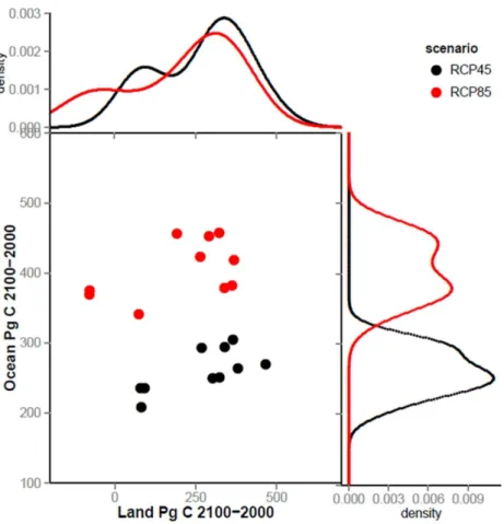
(Friedling-stein et al., 2006, 2014). Despite reduced uncertainty in the ocean projections, results from the subsequent fifth phase of Coupled Model Intercomparison Project (CMIP5, Taylor et al., 2012) also show a significant spread of land and ocean carbon future
pro-5
jections (Arora et al., 2013; Jones et al., 2013; Friedlingstein et al., 2014), as illustrated in Fig. 1. Note that for the land carbon projections, the spread due to model differences
is larger than difference across scenarios, highlighting again substantial uncertainty in
the projections because of land model uncertainties.
Following Friedlingstein et al. (2003), the change in atmospheric CO2 given
anthro-10
pogenic fossil fuel emissions (FF) is the result of the combined effects of the sensitivity
of the carbon cycle to climatic change (carbon-climate interaction, described asγL,γO, [D1]which are the land and ocean sensitivities, respectively) and the sensitivity of the carbon cycle to changes in the atmospheric CO2concentration (carbon-concentration interaction; described as βL,βO, which are the land and ocean sensitivities,
respec-15
tively; Friedlingstein et al., 2006; Gregory et al., 2009). While it has been long estab-lished that ambiguities in the representations of the physical aspects of the climate system contributes significantly to the overall uncertainties in climate projections (e.g. Bony et al., 2006; Knutti et al., 2008; Soden and Held, 2006), the C4MIP and CMIP5 results clearly demonstrate the importance of carbon-cycle climate interactions for
cli-20
mate projections (Gregory et al., 2009; Huntingford et al., 2009).
These carbon-cycle sensitivities have been used to characterise the climate-carbon feedback strength and have also been employed as a diagnostic tool to compare ESMs projections. For a given scenario, the land carbon-climate feedbacks for the CMIP5 models have been shown to be more uncertain than ocean feedback (Arora
25
BGD
11, 2083–2153, 2014Challenges and opportunities to reduce uncertainty in
projections
D. Dalmonech et al.
Title Page
Abstract Introduction
Conclusions References
Tables Figures
◭ ◮
◭ ◮
Back Close
Full Screen / Esc
Printer-friendly Version Interactive Discussion
Discussion
P
a
per
|
D
iscussion
P
a
per
|
Discussion
P
a
per
|
Discuss
ion
P
a
per
|
causes for the large spread in carbon-climate projections (Arora et al., 2013; Friedling-stein et al., 2006; Jones et al., 2013; Sitch et al., 2008), calls for a better understanding of the “real-world” carbon cycle sensitivities and their improved representation in Earth system models.
The terrestrial and marine biogeochemical components of Earth system models rely
5
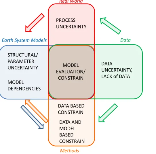
on “empirically-based” process representations to describe complex ecological pro-cesses at the larger spatial scale of these models. This adds significant uncertainties to an Earth system model, compared to the representation errors of physical atmo-sphere and ocean models, which are mainly associated with the parameterisation of physical processes occurring at subgrid-scale levels (Fig. 2). These ecological models
10
require extensive parameterization and/or upscaling procedures, however, despite con-siderable efforts, there are significant challenges to extrapolating empirical evidence
from controlled field or mesocosm experiments, which can address the carbon-cycle sensitivities of a particular ecosystem to the global scale (e.g. Zaehle et al., 2014). Pa-rameter and structural uncertainties of biological processes can be as much important
15
as physical-related uncertainties to the projected climate as indicated by single-model studies (e.g. Booth et al., 2012; Yurova et al., 2010).
In order to reduce uncertainties in coupled climate-carbon cycle model projections, these biogeochemical models need to be constrained by observational data, in a sim-ilar way as climate projections have been constrained in the past (e.g. Collins et al.,
20
2012; Knutti and Tomassini, 2008; Knutti et al., 2006; Sanderson and Knutti, 2012) (“methods” in Fig. 2). The key challenge is to turn the results and insights obtained due to the current trend to developing comprehensive benchmarking systems to eval-uate the terrestrial (Anav et al., 2013a; Cadule et al., 2010; Dalmonech and Zaehle, 2013; Luo et al., 2012; Piao et al., 2013; Randerson et al., 2009) and marine (Anav
25
BGD
11, 2083–2153, 2014Challenges and opportunities to reduce uncertainty in
projections
D. Dalmonech et al.
Title Page
Abstract Introduction
Conclusions References
Tables Figures
◭ ◮
◭ ◮
Back Close
Full Screen / Esc
Printer-friendly Version Interactive Discussion
Discussion
P
a
per
|
D
iscussion
P
a
per
|
Discussion
P
a
per
|
Discuss
ion
P
a
per
of current observational dataset (see Fig. 2), but also in-depth understanding of the processes and structures of the models under investigation.
The aim of this review is to assess and list key-issues and challenges that need to be taken into consideration if the uncertainties in future carbon-climate projections are to be reduced; with particular focus on the terrestrial and marine ecosystems component
5
of ESMs. We begin by discussing selected process uncertainties (Sects. 2 and 3). Key issues which impact the use of observations to constrain models are discussed in Sect. 4. Next, we discuss different levels of uncertainty that impact our ability to infer future
reliability of models based on their past/present-day performances (Sect. 5). Finally, we summarise key challenges and opportunity that can provide potential direction of
10
work.
2 Uncertainty in the marine ecosystem carbon cycle
2.1 Process uncertainties
The ocean-atmosphere net carbon exchange is primarily modulated by the physico-chemical reactions governing the solution of CO2 in water, and therefore the ocean
15
circulation, while biological processes play only a secondary role (Chavez et al., 2011; Le Quéré, 2010). A small fraction of the marine primary productivity of 40–50 Pg C yr−1
(PP; Behrenfeld and Falkowski, 1997; Longhurst et al., 1995) is exported to deeper ocean layers through sedimentation of dead biomass, providing a “biological pump” of CO2 into the ocean. Since marine production is limited by the availability of nitrogen,
20
phosphorus and silicon, this biological pump provides a coupling between the global cycle of silicon, nitrogen and phosphorus and the level of atmospheric CO2.
Currently, oceans take up roughly a quarter of the anthropogenic CO2 emissions,
primarily via the solution pump (Le Quéré et al., 2013). This ocean carbon sink over is likely to be altered in the next few decades due to the effects of climate changes
25
BGD
11, 2083–2153, 2014Challenges and opportunities to reduce uncertainty in
projections
D. Dalmonech et al.
Title Page
Abstract Introduction
Conclusions References
Tables Figures
◭ ◮
◭ ◮
Back Close
Full Screen / Esc
Printer-friendly Version Interactive Discussion
Discussion
P
a
per
|
D
iscussion
P
a
per
|
Discussion
P
a
per
|
Discuss
ion
P
a
per
|
1998), resulting in ocean surface warming and enhanced ocean stratification. These changes will impact the physico-chemical ocean C uptake, but also affect marine PP
through to altered nutrient and light availability associated with the direct effects of
temperature changes on production as well as the altered ocean circulation (Doney et al., 2004; Hallegraeff, 2010; Riebesell et al., 2009; Steinacher et al., 2010). While
5
there is generally consensus among several models on the leading role of the physico-chemical mechanisms, there remains substantial uncertainty as to the response of the biological related C uptake to e.g. temperature (e.g. Bopp et al., 2001; Steinacher et al., 2010).
There is substantial uncertainty in the understanding of the temperature response
10
of phytoplankton. Sarmiento et al. (2004) used an empirical model based on observa-tional constraints to predict a range of PP increase between 0.7–8.1 % by 2050 relative to pre-industrial conditions, depending on the algorithm used to describe the temper-ature sensitivity of PP. Using the UVic Earth System model, Taucher and Oschlies (2011) investigated the effect of the temperature sensitivity of PP relative to the
con-15
tribution of temperature-induced circulation changes. They showed that accounting for the temperature sensitivity of PP led to a different sign of the projected PP change.
One reason for the uncertainty on the temperature response of marine PP is that it is unclear, how temperature will affect the structure of the phytoplankton communities.
Thomas et al. (2012) suggested that phytoplankton might show adaptive behaviour
20
with respect to optimum of temperature. Recent attention has therefore moved towards understanding the impact of changes in the community structure and its impact along the food chain. However, uncertainty for instance related to different temperature
sensi-tivities within the community, in terms of growth rate and grow efficiency and interacting
effects, does not allow to quantify the strength and the persistence of feedbacks with
25
climate (Riebesell et al., 2009). While therefore potential changes are to be expected for the future, the net effect on the total functionality is still unknown.
The other important effect of increasing atmospheric CO2 levels, and thus the
con-BGD
11, 2083–2153, 2014Challenges and opportunities to reduce uncertainty in
projections
D. Dalmonech et al.
Title Page
Abstract Introduction
Conclusions References
Tables Figures
◭ ◮
◭ ◮
Back Close
Full Screen / Esc
Printer-friendly Version Interactive Discussion
Discussion
P
a
per
|
D
iscussion
P
a
per
|
Discussion
P
a
per
|
Discuss
ion
P
a
per
current a shift in the seawater carbonate chemistry, shifting inorganic carbon from car-bonate toward more bicarcar-bonate and CO2 (Doney et al., 2009a). The biological
con-sequences of ocean acidification are not well understood globally, as both positive and negative responses have been observed among different groups of marine organisms
in biological data (Langdon et al., 2003; Malakoff, 2012; Riebesell et al., 2007). The
5
number of ocean acidification studies conducted at relevant CO2 levels is still limited
(Fabry et al., 2008). Furthermore, the currently available experiments are limited to short term laboratory experiments, hence not compatible with expected rate of change in concentration of CO2. This is relevant because of the potential for the community to
adapt to new pH conditions at the time-scale of the anthropogenic CO2 perturbation
10
(Doney et al., 2009a). Furthermore, simulating future impacts of ocean acidification on marine biology requires assumptions to be made on changing C : N : P stoichiometry (see next paragraph), which cannot be accounted for in current generation models that assume fixed C : N : P ratios (Tagliabue et al., 2011). As research on ocean acidification is a relatively new field of research, predicting its impacts still presents a challenge to
15
the biogeochemical modelling community.
The marine nitrogen cycle plays a central role in ocean biogeochemistry as a limiting nutrient for PP. Global PP depends on the amount of bioavailable nitrogen, which in turn depends on the biological processes of nitrogen-fixation and denitrification. While feed-backs within the marine nitrogen cycle are mediated by the phosphorus cycle, through
20
the N : P ratio in surface water (Gruber, 2008), uncertainties in future evolution of the marine nitrogen cycle will also centre on the possibility of a decrease in oxygen con-centration in the ocean interior, which would increase denitrification and subsequently lower PP (Gruber, 2008). The future evolution of the marine nitrogen cycle will depend on ocean circulation and on changes in aeolian iron availability (Berman-Frank et al.,
25
2008).
It is clear that the physical change and the solubility pump will have a significant con-tribution in determining the ocean net CO2 fluxes for the decades to come (Denman
BGD
11, 2083–2153, 2014Challenges and opportunities to reduce uncertainty in
projections
D. Dalmonech et al.
Title Page
Abstract Introduction
Conclusions References
Tables Figures
◭ ◮
◭ ◮
Back Close
Full Screen / Esc
Printer-friendly Version Interactive Discussion
Discussion
P
a
per
|
D
iscussion
P
a
per
|
Discussion
P
a
per
|
Discuss
ion
P
a
per
|
role that marine bacterial community could play in the future, if climate-change induced changes in the rate of marine PP propagates into significant changes of the biolog-ical pump. For instance, Schmittner et al. (2008) have demonstrated in a modelling experiment that changes in the marine PP affecting the biological pump may become
important for the net ocean carbon uptake on centennial to millennial time scale.
5
2.2 Intra- and inter-model uncertainties
The spread in the projections of the ocean carbon cycle and its climate-CO2feedbacks
in current ESMs has been shown to be not negligible, but less large than the spread of projections of the corresponding land models (Arora et al., 2013). Uncertainties arise in simulating future ocean biogeochemical cycles for a wide variety of reasons, linked
10
to how the physics and the biology of the system is represented (Doney et al., 2004; Gnanadesikan et al., 2004; Sarmiento et al., 2004). Efforts toward the development
of a more process-based representation of ocean trophic dynamics have increased in the last decade, allowing linkages to be made between the ocean physical process of transport and the process of marine primary productivity (Dutkiewicz et al., 2009; Le
15
Quere et al., 2005). Previously, few studies used prognostic models to determine the response of ocean biology to warming (e.g. Bopp et al., 2001; Boyd and Doney, 2002). Ocean physics and biology are tightly coupled and uncertainties in the physic of the system translate in uncertainties in the biological counterpart. Figure 3 reports the global scores computed by Anav et al. (2013a) and used to rank the ESMs
participat-20
ing to the CMIP5. These scores represent the global performance under present-day conditions with respect to climate and ocean global variables and component of the carbon cycle (we excluded the net carbon fluxes) for ocean and land. Seasonalities, interannual variability and stocks of key-variables are considered. For each variable Fig. 3a reports the standard deviation computed among the models performances.
25
Since all the scores range between 0 and 1 (skilful model), the standard deviation can be compared and indicates for which variables the models differ the most in terms of
vari-BGD
11, 2083–2153, 2014Challenges and opportunities to reduce uncertainty in
projections
D. Dalmonech et al.
Title Page
Abstract Introduction
Conclusions References
Tables Figures
◭ ◮
◭ ◮
Back Close
Full Screen / Esc
Printer-friendly Version Interactive Discussion
Discussion
P
a
per
|
D
iscussion
P
a
per
|
Discussion
P
a
per
|
Discuss
ion
P
a
per
ables of the systems (i.e. sea-surface temperature, SST; mixing-layer depth, MLD) and biological variables (i.e. PP) are important to explain the between-model differences. In
the same figure, the lower panel reports also the actual scores for each ESM realization (Fig. 3c).
Biogeochemical ocean models show a large disagreement on projected changes in
5
future PP, with uncertainties in the magnitude of change. Even when models agree globally on the sign of change, regional differences in projected PP exist (Steinacher
et al., 2010). A multi-model study by Steinacher et al. (2010) using four ESMs showed a decrease in global mean PP of between 2 and 20 % by 2100 relative to pre-industrial conditions under SRES A2 emission scenario, while Schmittner et al. (2008) using
an-10
other ESM (UVic) found that global PP increases by 2100 following the same emission scenario. Bopp et al. (2013) showed that the differences of the CMIP5 projections of
global and regional changes in PP are not as robust across ESMs, as sea surface temperature and pH.
One cause of the diverging projections are model parameterisations of processes,
15
which cannot be represented explicitly at the spatial and temporal scale of the model (e.g. meso-scale eddies), or for which insufficient knowledge is available to explicitly
model these processes (e.g. effects of marine biodiversity on carbon cycling). The way
in which mesoscale eddies are modelled has a significant effect on the vertical supply
of nutrients, and therefore, biological activity and PP (Chelton et al., 2011; Oschlies
20
and Garçon, 1998).
Biogeochemical cycling is also highly dependent upon specific plankton functional types (PFTs) and the explicit inclusion of PFTs in models is needed to take ecological changes into account (Le Quere et al., 2005). However, incorporating PFTs into models may add further uncertainty to the model if additional model parameters remain insuffi
-25
BGD
11, 2083–2153, 2014Challenges and opportunities to reduce uncertainty in
projections
D. Dalmonech et al.
Title Page
Abstract Introduction
Conclusions References
Tables Figures
◭ ◮
◭ ◮
Back Close
Full Screen / Esc
Printer-friendly Version Interactive Discussion
Discussion
P
a
per
|
D
iscussion
P
a
per
|
Discussion
P
a
per
|
Discuss
ion
P
a
per
|
Sailley et al. (2013) showed that the model structure in four different models that
in-clude PFTs has a large effect on the governing mechanisms responsible for variations
in plankton biomass. Oschlies (2001) showed that different ecosystem model
configu-rations have a large effect on primary production based on element recycling, and thus
total PP. However Friedrichs et al. (2009) showed that increasing model complexity
5
does not increase the model skill in simulating PP.
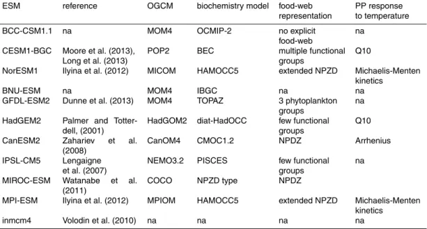
Compared to ocean physical dynamics and ocean chemistry, less is known about the response of marine biology to climate and atmospheric CO2and changes. This is
reflected by a lower degree of complexity in ocean biological models, compared to the richness of interacting biological processes in terrestrial ecosystem models. Table 1
10
identifies common sub-components of the models used in the CMIP5 project, as for in-stance same ocean circulation models for some ESMs or similar food-web structures. Due to better predictability of the physico-chemical effects and the lower importance of
biological processes, the future patterns of ocean-atmosphere are relatively more com-parable among models and the spread is smaller compared to land models, as shown
15
in Fig. 1. There is a potential that the simplicity of the ocean biological models prevents a full assessment of the possible feedbacks betweenpCO2, temperature and biologi-cal C uptake, hence when and with which degree the marine biologibiologi-cal component can provide a feedback in the carbon-climate system is still hence an open issue.
3 Uncertainty in the terrestrial carbon cycle
20
3.1 Process uncertainties
The net CO2 exchange of terrestrial ecosystems is controlled by the activity of
veg-etation and soil organisms and their respective responses to climate and CO2
con-centration perturbations (Chapin III et al., 2009; Davidson and Janssens, 2006). An-thropogenic land-use and land-use change (Houghton et al., 2012), and natural
dis-25
BGD
11, 2083–2153, 2014Challenges and opportunities to reduce uncertainty in
projections
D. Dalmonech et al.
Title Page
Abstract Introduction
Conclusions References
Tables Figures
◭ ◮
◭ ◮
Back Close
Full Screen / Esc
Printer-friendly Version Interactive Discussion
Discussion
P
a
per
|
D
iscussion
P
a
per
|
Discussion
P
a
per
|
Discuss
ion
P
a
per
which currently absorbs about a quarter of the anthropogenic CO2emission (Le Quere et al., 2013).
Here we focus on the most important, biologically controlled processes, which shape the macroscopic, decadal to century scale evolution of the net land carbon balance, be-cause of their strong dependence of climate and atmospheric CO2levels, and thus their
5
potential to give rise to land-atmospheric CO2feedbacks: (i) the response of
photosyn-thesis to elevate CO2and its potential down-regulation (Lloyd and Farquhar, 2008) ; (ii) acclimation of plant carbon uptake and release to increasing temperature (Lloyd and Farquhar, 2008); (iii) acclimation of soil fauna, microbial and fungal activity to tempera-ture (Craine et al., 2012).
10
The gross assimilation of carbon into plants responds strongly positive to ele-vated CO2at short-time scales (Ainsworth and Long, 2005). This short-term response
is encoded into current ESMs and the cause for the large negative land carbon-concentration feedback (Arora et al., 2013). However, plants may down-regulate photo-synthesis under increasing CO2acting on physiological and biochemical adjustments.
15
In addition, changes in the allocation of the assimilated carbon between short-lived (leaves, fine roots) and longer-lived (wood) tissues may alter the net C storage of plants (and ecosystems) to elevated CO2 (Körner et al., 2005; Luo et al., 2003). Next
to the carbon balance of the plants, these changes in allocation, specifically the total belowground carbon flux affect also the soil organic matter dynamics. However, these
20
characterized by significant complexity and the mechanisms explaining the interactions between these fluxes with variability in soil moisture and temperature are at the current state not enough understood (Chaplin et al., 2009).
Consequently, experimental studies indicate a wide range of responses of plant biomass to increasing atmospheric CO2, dependent on species and experimental
con-25
ditions (e.g. Poorter and Navas, 2003). Differences in CO
2response can in some cases
mod-BGD
11, 2083–2153, 2014Challenges and opportunities to reduce uncertainty in
projections
D. Dalmonech et al.
Title Page
Abstract Introduction
Conclusions References
Tables Figures
◭ ◮
◭ ◮
Back Close
Full Screen / Esc
Printer-friendly Version Interactive Discussion
Discussion
P
a
per
|
D
iscussion
P
a
per
|
Discussion
P
a
per
|
Discuss
ion
P
a
per
|
els could improve realism and reduce uncertainties. However, the complexity of the responses of plants to elevated CO2 make difficult to identify the overarching
mecha-nisms, and thus to sufficiently constrain the response of the net plant carbon balance
to CO2(Zaehle et al., 2014).
Photosynthesis, as well as plant and soil respiration increase instantaneously with
5
temperature as long as the temperature remains below a critical temperature threshold (e.g. Lloyd and Taylor, 1994). This response is implemented in the current regener-ation of ESMs, and gives rise to the positive carbon-climate interaction (Arora et al., 2013). However, acclimation of the response has been observed in many cases, in-volving several mechanisms at the tissue-level and organ level (see the review of Smith
10
and Dukes, 2013). Acclimation of photosynthesis to temperature has been observed in several species (Kositsup et al., 2008; Way and Sage, 2008) and may strongly attenu-ate the plant’s temperature response. However no general pattern of photosynthesis– temperature relationships has emerged, as data are available only at local scale and vary strongly between experiments. Consequently, few models have included such
pa-15
rameterisation (see e.g. Smith and Dukes, 2013).
Similarly to photosynthesis, plants might adjust their respiratory rate in response to changes in temperature, influenced also by other factors such as light or availability of nutrients (Atkin and Tjoelker, 2003; Atkin et al., 2005). The fairly poor understand-ing of acclimation and adaptation mechanisms at biochemistry level due to potential
20
confounding factors (i.e. vapour pressure deficit), contributes to the lack of robust pre-dictability (Lin et al., 2012). Nevertheless, Ziehn et al. (2011) identified temperature acclimation of photosynthesis and respiration, as well as the stomatal response to CO2 as explaining factors for the residual variation in the net photosynthetic rate after the assimilation of leaf-trait in the BETHY model, highlighting the importance of constrain
25
these mechanisms.
BGD
11, 2083–2153, 2014Challenges and opportunities to reduce uncertainty in
projections
D. Dalmonech et al.
Title Page
Abstract Introduction
Conclusions References
Tables Figures
◭ ◮
◭ ◮
Back Close
Full Screen / Esc
Printer-friendly Version Interactive Discussion
Discussion
P
a
per
|
D
iscussion
P
a
per
|
Discussion
P
a
per
|
Discuss
ion
P
a
per
Zhou et al., 2011). The response is further complicated changes in substrate availabil-ity for soil organic matter decomposition, as substrate limitation might cause appar-ent lower temperature sensitivity e.g. (Holland et al., 2000). Progress has been made to simulate the response of microbial activity to altered substrate availability (Wielder et al., 2013). Similarly, the role of soil vertical transport of organic matter might have
5
important implications for the stock of carbon on the long term through stabilisation mechanisms along soil depth (Braakhekke et al., 2011). However, the implication of these processes for global carbon storage has not been fully explored by global mod-els. Soil incubation experiments are typically not long enough to strongly support either hypothesis and thus to provide a constraint for soil C models. There is hence the need
10
to provide more comprehensive studies on the interactive effect of temperature and
labile carbon availability on soil respiration (Davidson and Janssens, 2006).
Uncertainties in the future response of terrestrial C store to climate change arise also from other processes. Thawing permafrost will potentially release a large amount of carbon due to warming, however, there is large uncertainty about the timing and
15
magnitude of this C flux (e.g. MacDougall et al., 2012). Although globally applicable permafrost soil models exist, none of the CMIP5 models include a representation of permafrost carbon and its potential positive climate-carbon feedback. Hence the role of carbon release from permafrost areas due to warming is still to be quantified in a coupled setting.
20
Despite the fact that functional biodiversity is better represented in terrestrial than marine ecosystem models, current global vegetation models typically fail to realistically consider demographic processes and the true diversity of plant types (Purves and Pacala, 2008; Friend et al., 2013). Rates of recruitment, competitive interactions, and rates of mortality are all likely to change as a result of future environmental change,
25
vegeta-BGD
11, 2083–2153, 2014Challenges and opportunities to reduce uncertainty in
projections
D. Dalmonech et al.
Title Page
Abstract Introduction
Conclusions References
Tables Figures
◭ ◮
◭ ◮
Back Close
Full Screen / Esc
Printer-friendly Version Interactive Discussion
Discussion
P
a
per
|
D
iscussion
P
a
per
|
Discussion
P
a
per
|
Discuss
ion
P
a
per
|
tion, and mortality rates in particular are strongly dependent on species and environ-mental conditions (Lines et al., 2010). There is therefore an urgent need to explore approaches for incorporating more realistic demographic approaches into global vege-tation models, and investigating their consequences.
The constraints on carbon cycling imposed by the cycles of macro-nutrients such as
5
nitrogen and phosphorus have been shown to limit the potential of land to sequester more carbon in response to increasing atmospheric CO2 (Oren et al., 2001; Norby
et al., 2010; Hungate et al., 2013; Zaehle et al., 2014), while alleviating only little of ter-restrial N limitation in response to warming (Melillo et al., 2011; Zaehle and Dalmonech, 2011). However, carbon-nitrogen interactions and feedbacks are only included in few
10
ESMs (Zaehle and Dalmonech, 2011). Also, the impact of tropospheric ozone on veg-etation (Anav et al., 2011; Sitch et al., 2007) is not yet simulated by ESMs.
3.2 Intra- and inter-model uncertainties
Terrestrial ecological dynamics are currently represented with diverging degree of de-tail in terms of structures, terrestrial-climate biophysical interactions and response to
15
disturbances. Contrary to marine ecosystems (Sect. 2.2), in which physics and biol-ogy of the ocean are tightly linked, differences amongst terrestrial ecosystem models
in ESMs are caused primarily because of alternative representations of carbon-cycle processes, rather than the representation of land biophysics. Similarly to ocean mod-els, Fig. 3b shows for which global land variables the models performance diverge the
20
most. Most of the spread in the model performances is associated to global land C-related variables across ESMs (i.e. GPP, global soil and vegetation C stocks), while for climate variables, models are relatively closer in terms of performance, hence less uncertain compared to C-related variables. The spread of performance referred to soil C stock is related to a clear cluster of model realizations as also emerging from Fig. 3d.
25
Anav et al. (2013a) found that the range of GPP simulated by ESMs for the present day varies between 113 and 178 Pg C yr−1. Piao et al. (2013) obtained a similar result
cli-BGD
11, 2083–2153, 2014Challenges and opportunities to reduce uncertainty in
projections
D. Dalmonech et al.
Title Page
Abstract Introduction
Conclusions References
Tables Figures
◭ ◮
◭ ◮
Back Close
Full Screen / Esc
Printer-friendly Version Interactive Discussion
Discussion
P
a
per
|
D
iscussion
P
a
per
|
Discussion
P
a
per
|
Discuss
ion
P
a
per
mate, which ranged between 110 and 150 Pg C yr−1. For two particular models, Piao
et al., 2013 show that the difference in GPP between offline and online varied up to
20 Pg C yr−1 as result of the bias in the simulated climate and as result of the
cou-pling. Large variability at the present day is also reported for soil carbon content, with some ESMs having a low limit of about 500 Pg C yr−1 and other having values up to
5
3000 Pg C yr−1(Anav et al., 2013a; Todd-Brown et al., 2012).
These differences depicted for present-day conditions must translate in differences
under future scenario. Model responses under future scenarios have been already shown to vary largely amongst terrestrial models outcome in both offline (e.g. Cramer
et al., 2001; Sitch et al., 2008) and within ESMs (Arora et al., 2013; Friedlingstein et al.,
10
2006), as several of these terrestrial ecosystem models are also included in coupled climate models.
Previous analysis of the C4MIP models output showed strong model divergence in predicted trajectories of land carbon storage, in some cases with disagreement on the sign of changes in vegetation and soil carbon pools response globally
(Friedling-15
stein et al., 2006) and regionally (e.g. Qian et al., 2010; Sitch et al., 2008). Arora and Matthews (2009) fitted the global parameters of a carbon box model to each ESMs of the C4MIP project, in order to provide a common standard to compare processes, oth-erwise differently modelled in each single ESM. Despite the fitted parameters contain
implicitly the information on the modelled climate of each ESMs, the analysis revealed
20
the lack of consensus among models in terms of magnitude of response of NPP to CO2and climate change, but also of vegetation and soil carbon turnover rate.
At regional scales, several published modelling studies agree on the pivotal role of the tropical latitudinal band in the global carbon cycle in response to climate variabil-ity both at present e.g. (Jones et al., 2001; Zeng et al., 2005) and in the future (Cox
25
BGD
11, 2083–2153, 2014Challenges and opportunities to reduce uncertainty in
projections
D. Dalmonech et al.
Title Page
Abstract Introduction
Conclusions References
Tables Figures
◭ ◮
◭ ◮
Back Close
Full Screen / Esc
Printer-friendly Version Interactive Discussion
Discussion
P
a
per
|
D
iscussion
P
a
per
|
Discussion
P
a
per
|
Discuss
ion
P
a
per
|
However, land surface models differ in the simulation of the impact of occurrence of
drought conditions on tropical vegetation. Under strong drying of the Amazon Basin, several vegetation models showed that the chance for a forest dieback will increase in the future. However, the likelihood of occurrence of this tipping point depends strongly on the model of vegetation (Huntingford et al., 2008; Poulter et al., 2010), the plant
5
physiological responses (Fisher et al., 2010; Galbraith et al., 2010; Huntingford et al., 2013) and the extend of predicted drying (Huntingford et al., 2013; Malhi et al., 2009; Shiogama et al., 2011).
Similarly to Hungtinford et al. (2013), several studies indicate the dominance of un-certainties attributable to parameters such as temperature-photosynthesis response,
10
in tropical areas (e.g. Matthew et al., 2007; Booth et al., 2012). Booth et al. (2012) in particular found a large range of possible values of the parameters regulating the op-tima in the temperature–photosynthesis relationship compatible with the atmospheric CO2for present day.
Modelled soil carbon processes are also key contributors to the uncertainty of carbon
15
patterns, both between models (e.g. Qian et al., 2011) and within model (e.g. Zaehle et al., 2005). The experiments of (Jones et al., 2005) and (Thum et al., 2011), in which different soil model structures were explored in terms of response to climate change,
showed how a difference in the model might affect the magnitude of the carbon-climate
feedback strength of the carbon sensitivity and climate-carbon feedbacks affecting the
20
response of soil respiration and hence the magnitude of the carbon release. Yurova et al. (2009) used three different soil structures, according to three different conceptual,
state-of-the-art approaches. They showed that the resultant uncertainty in projected climate change are comparable to the modelled temperature differences, which are
due to the carbon-climate interaction in C4MIP models (Zeng et al., 2004).
25
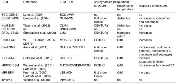
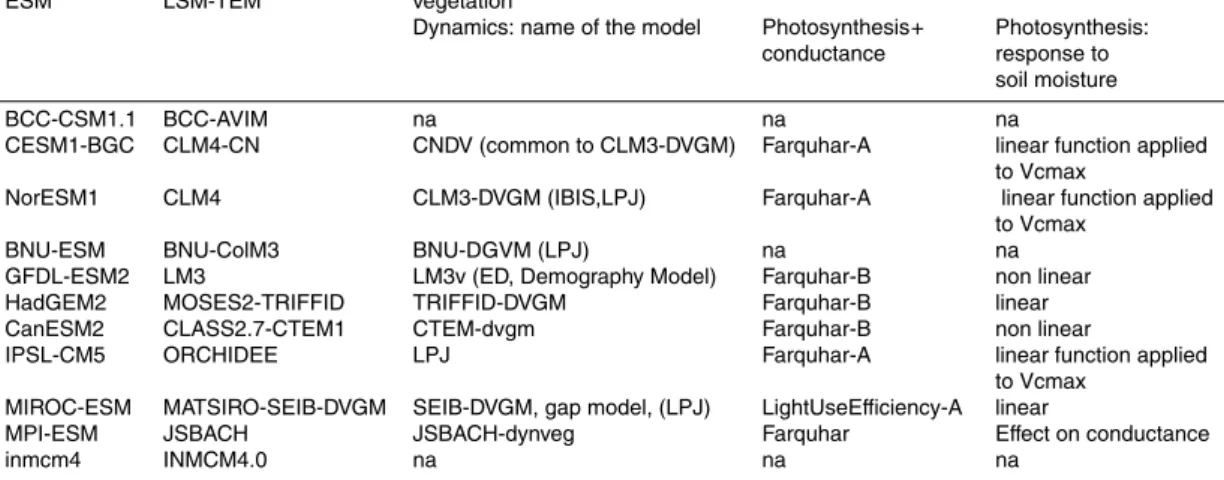
As for marine ecosystem models, Tables 2 and 3 report how processes such as soil respiration and the temperature and drought effects on photosynthesis and canopy
BGD
11, 2083–2153, 2014Challenges and opportunities to reduce uncertainty in
projections
D. Dalmonech et al.
Title Page
Abstract Introduction
Conclusions References
Tables Figures
◭ ◮
◭ ◮
Back Close
Full Screen / Esc
Printer-friendly Version Interactive Discussion
Discussion
P
a
per
|
D
iscussion
P
a
per
|
Discussion
P
a
per
|
Discuss
ion
P
a
per
most of the current ESMs use also the soil dynamics represented in the Century model (Parton et al., 1993).
It is not possible to obtain full descriptions of the main structures and key param-eterisations for all the models. Tables 2 and 3 report the main sub-units, and key-models used as reference for parameterization or structures. The degree of common
5
model structures indicated in Tables 2 and 3 shows that the projections of these mod-els might not be completely independent information. Given the above discussion, it clearly emerges that the current ensemble used in CMIP5 does not sample the entire possible space of climate responses of soil processes.
4 Constraining future projections based on observations: data and metrics
10
Given the divergence of model outcomes for the contemporary period (Anav et al., 2013) and in the future (e.g. Bopp et al., 2013; Jones et al., 2013), it is imperative to have a good understanding of the available, appropriate datasets and methodol-ogy to evaluate models (Foley et al., 2013). The development of a constraint based on observations should benefit from the richness of available datasets. Nevertheless,
15
uncertainties of the data set and their use as a constraint may limit the application of a particular data set as a constraint. Some of these uncertainties and/or limits are also common to the general model evaluation and calibration problems, such as data un-certainties (see the review of Foley et al., 2013). In this section we discuss examples and key-issues related to (i) observational constraint; (ii) selection of the appropriate
20
dataset; and (iii) performance metrics.
4.1 Observational constraints
Terrestrial and marine ecosystem models are expected to return characteristics of the system such as the average state of the system (hereafter “climatology”), and evalua-tion exercise targeting this climatology are fundamental to pinpoint model weaknesses
BGD
11, 2083–2153, 2014Challenges and opportunities to reduce uncertainty in
projections
D. Dalmonech et al.
Title Page
Abstract Introduction
Conclusions References
Tables Figures
◭ ◮
◭ ◮
Back Close
Full Screen / Esc
Printer-friendly Version Interactive Discussion
Discussion
P
a
per
|
D
iscussion
P
a
per
|
Discussion
P
a
per
|
Discuss
ion
P
a
per
|
and consecutively improve the model. However, such an evaluation does not neces-sarily translate into a constraint for the model’s capacity to make projections. An obser-vational constraint should have a strong relationship with a forecast quantity of interest (e.g. the carbon storage in 2100) and should contain a detectable trend or predictable variability, such as an anthropogenic-induced signal (Allen et al., 2000). In other words,
5
model evaluation has to be performed with respect not only to climatology, but also the carbon dynamics that are likely to be important to predict the impact of climate change and increasing atmospheric CO2on land and marine ecosystems. An example for this
would be an observational constraint, which has a clear relationship between the mea-sure of model error (here indicated with the general term “model-data” distance) and
10
the magnitude of the carbon-climate feedback.
The point related to the anthropogenic-induced signal can be solved having long temporal series of the observed quantity, where it is possible to assess that apparent trends in the data are not caused by long-time scale, but natural and system inherent variability. That is the case for long-term records of temperature (Gillett et al., 2012;
15
Rowlands et al., 2012) but is a challenge for shorter datasets, as demonstrated by (Henson et al., 2010). Nevertheless, it is important to detect features in the data that highlight underlying trends, such as the sensitivity of processes/variables to particular drivers, that we know they will be impacted in the future, as for instance evidenced in ecosystem manipulation studies. This approach assumes that the ecosystem will have
20
a response in the future, which is comparable to its present-day sensitivity to that driver. Atmospheric CO2 records from ice cores and monitoring stations (continuous and
flask data), Table 4, are one of the observational datasets most commonly used to evaluate and constrain the simulated carbon cycle in terms of climatology, but also trends and sensitivities (Cadule et al., 2010; Dalmonech and Zaehle, 2013; Dargaville
25
BGD
11, 2083–2153, 2014Challenges and opportunities to reduce uncertainty in
projections
D. Dalmonech et al.
Title Page
Abstract Introduction
Conclusions References
Tables Figures
◭ ◮
◭ ◮
Back Close
Full Screen / Esc
Printer-friendly Version Interactive Discussion
Discussion
P
a
per
|
D
iscussion
P
a
per
|
Discussion
P
a
per
|
Discuss
ion
P
a
per
change in atmospheric CO2 as response to a change in global temperature can be used as a combined constraint onγ[D2] andβ(Cox and Jones, 2008; Gregory et al., 2009; Scheffer et al., 2006).
Longer-time scale constraints require indirect measurements of changes in atmo-spheric CO2, such as derived from ice-cores. Using records of the temperature and
5
CO2 drop during the little ice age, 1500–1750 AD Cox and Jones, (2008) estimated
values of the global carbon-cycle sensitivity to climate as high as 40 ppmv◦C−1. Frank
et al. (2010) instead, using ensemble reconstructions of the past millennium, estimated the range as 1.7–21.4 ppmv◦C−1
(median of 7.7 ppmv◦C−1
), against the estimated modeled range of 2.1–15.6 ppmv◦C−1
from the C4MIP models. The values calculated
10
by Cox and Jones (2008) are assumed to be representative of the global sensitivity at centennial to multi-centennial scales, hence comparable to the carbon-climate projec-tions for the next century. (Frank et al., 2010) instead used the values as representative of the 20th century climate perturbation (the historical 0.7◦C increase of temperature).
However, these sensitivities could show a time scale-dependency (Friedlingstein and
15
Prentice, 2010; Woodwell et al., 1998; Willeit et al., 2014). In other words, the re-sponse to external drivers has its own temporal scale, which is the result of aggregated subcomponent responses of the ecosystems that act differently with different time
re-sponse. This may also depend with magnitude of change, for instance on the rate of warming, the rate of CO2increase and the initial conditions, hence the state of the
sys-20
tem e.g. (Gregory et al., 2009; Shaver et al., 2000). These points might have several implications:
Firstly, the evaluation is often performed at a specific level of aggregation of the mod-elled process (i.e. land NPP or ocean PP response to a particular stressor). However, these data do not always detect only the signal of interest (e.g. a pure climate or pure
25
CO2 effect) on the specific process, because of internal feedbacks or confounding
BGD
11, 2083–2153, 2014Challenges and opportunities to reduce uncertainty in
projections
D. Dalmonech et al.
Title Page
Abstract Introduction
Conclusions References
Tables Figures
◭ ◮
◭ ◮
Back Close
Full Screen / Esc
Printer-friendly Version Interactive Discussion
Discussion
P
a
per
|
D
iscussion
P
a
per
|
Discussion
P
a
per
|
Discuss
ion
P
a
per
|
Secondly, if the sensitivities are state-dependent, it will be important for models to also correctly return the state of the system along to the slope of the sensitivity, which will be difficult in the case of processes acting on longer time scales, such as vegetation
rebound from past disturbance, the extent of nutrient limitation, or gradual changes in the biophysical boundary conditions.
5
Lastly, the occurrence of different ecological response time scales indicates that the
model evaluation and the formulation of model constraints needs to address the dy-namics at the process level, and a relevant temporal and spatial scales, which help as-sess internal feedbacks of the system (Cox et al., 2013). Due to inherent non-linearities in the system, the short scale processes can have hence an impact also on longer
10
temporal scales relevant for the future carbon-climate evolution (Cox et al., 2013, see Sect. 5.2.1).
4.2 Global dataset
4.2.1 Terrestrial dataset
There is a large data-base of derived datasets, benefitting of extensive spatial and
15
temporal coverage (Table 4, see also Luo et al., 2012 for terrestrial data sets). Along to the already mentioned dataset, a CO2 net land and ocean fluxes database based on
inversions (Table 4), is available as a result of the TransCom3 project (Gurney et al., 2002) and it has been recently used to evaluate the ESMs participating to the CMIP5 (Anav et al., 2013a). Satellite-based dataset have been successfully used to evaluate
20
marine and terrestrial ecosystem in several regions and over the globe (Anav et al., 2013b; Dalmonech and Zaehle, 2013; Friedrichs et al., 2009; Guenet et al., 2013; Kelley et al., 2013; Randerson et al., 2009) and we can benefit of record of up to almost 30 yr of data.
Compared to most of the satellite dataset, that are related mainly to phenology or leaf
25
BGD
11, 2083–2153, 2014Challenges and opportunities to reduce uncertainty in
projections
D. Dalmonech et al.
Title Page
Abstract Introduction
Conclusions References
Tables Figures
◭ ◮
◭ ◮
Back Close
Full Screen / Esc
Printer-friendly Version Interactive Discussion
Discussion
P
a
per
|
D
iscussion
P
a
per
|
Discussion
P
a
per
|
Discuss
ion
P
a
per
carbon-process. While satellite-based datasets provide information only for the surface layer and for limited biological properties, they could be used in combination with other datasets such as vegetation height measurements (Simard et al., 2011).
Global up-scaled records as the GPP-product by (Jung et al., 2011), soil respira-tion (e.g. Bond-lamberty and Thomson, 2010), soil carbon (e.g. Nachtergaele et al.,
5
2012; FAO 2009) and vegetation carbon stocks (e.g. Gibbs et al., 2006) are valuable datasets to evaluate the “climatology” of the carbon cycle. Nevertheless caution has to be used when these dataset are implemented for a quantitative constraint, due to the inherent uncertainties associated to the upscaled procedure and the lack of a temporal dimension with which to assess current trends.
10
Currently, tropical areas lack of extensive in situ “observational” records, including manipulative experiments (Luo et al., 2006) and leaves traits (Kattge et al., 2011). This is fundamental in order to e.g. understand how fertilisation effect might counteract
the direct effect of temperature on plant physiological response, and hence supporting
plant resilience.
15
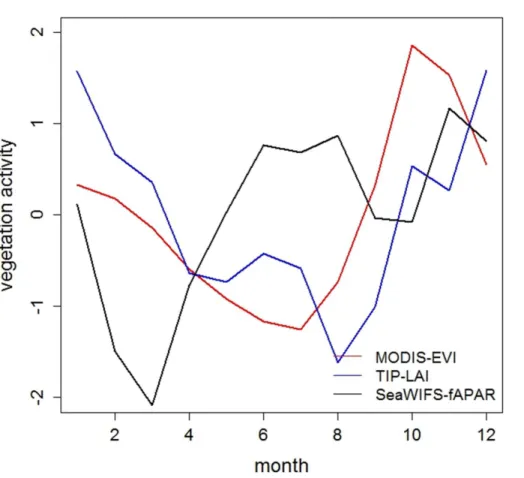
Satellite based data are also affected by high uncertainties in tropical areas (Asner
and Alencar, 2010). As an example, Fig. 4 reports the standardised seasonal signal of selected satellite-based datasets of vegetation activity aggregated over the Amazon area (Appendix A). The figure shows the lack of agreement between different records in
depicting the same underlying process and obstacles the selection of the most suitable
20
dataset and hence the evaluation and constrain exercise. Similarly, derived dataset of net CO2fluxes obtained by inversions, despite their usefulness to highlight differences
when aggregated by latitudinal band, might be a poor constrain on the tropical latitudi-nal band due to the paucity of CO2monitoring stations used in the inversion processes.
For instance, Koffiet al. (2012) assimilated data of atmospheric CO2to constrain GPP
25
BGD
11, 2083–2153, 2014Challenges and opportunities to reduce uncertainty in
projections
D. Dalmonech et al.
Title Page
Abstract Introduction
Conclusions References
Tables Figures
◭ ◮
◭ ◮
Back Close
Full Screen / Esc
Printer-friendly Version Interactive Discussion
Discussion
P
a
per
|
D
iscussion
P
a
per
|
Discussion
P
a
per
|
Discuss
ion
P
a
per
|
4.2.2 Marine dataset
Similarly as for land, TransCom 3 provides ocean air–sea CO2 fluxes database
(Ta-ble 4). The new Surface ocean CO2Atlas (SOCAT) aims to provide a comprehensive,
publicly available, regularly updated global dataset of marine CO2which is independent from the Takahashi database (Pfeil et al., 2012) (Table 4).
5
Global scale estimates of variables such as chlorophyll a and diffuse attenuation
coefficient are available from remotely sensed measurements from the Coastal Zone
Color Scanner (1978–1986), Sea-viewing Wide Field-of-view Sensor (1997–2010) and Aqua Modis (2002–2012). For marine ecosystems, the physical and the biological parts are tightly coupled and this makes the evaluation and constrain of the biological
sub-10
components difficult. For example, in Fig. 5 the timing of the blooming of chlorophyll
concentration has been computed for SeaWifs-based dataset. Although this is a robust observational feature linked to the phenology of marine PP, such information is linked not only to the marine ecosystem but also to the modelled physical ocean system via the vertical mixing. Therefore, this biogeochemical metric can be viewed as a way to
15
support a joint constrain of circulation and biogeochemistry models.
New marine dataset will allows to explore, along to stock data, information at com-munity structural level and physiological level. The new MAREDAT (MARine Ecosys-tem DATa) database (Buitenhuis et al., 2013) provides one of the first comprehensive biomass datasets to validate plankton in the ocean. The initiative provides global
grid-20
ded data for 11 plankton functional types (PFTs) including 9 of the PFTs that have been proposed as essential in simulating important biogeochemical processes in the oceans (Le Quéré et al., 2005). In addition new dataset providing information such phytoplankton physiological parameters are becoming available (Barton et al., 2013; Litchman and Klausmeier, 2008; Thomas et al., 2012).
BGD
11, 2083–2153, 2014Challenges and opportunities to reduce uncertainty in
projections
D. Dalmonech et al.
Title Page
Abstract Introduction
Conclusions References
Tables Figures
◭ ◮
◭ ◮
Back Close
Full Screen / Esc
Printer-friendly Version Interactive Discussion
Discussion
P
a
per
|
D
iscussion
P
a
per
|
Discussion
P
a
per
|
Discuss
ion
P
a
per
4.3 Metrics
Evaluation metrics can be used to synthesise the complexity of model-data compari-son, and thereby to facilitate comparing and ranking the models, as well as formulating weights to provide probabilistic forecast in multi-model ensemble and perturbed en-semble (Sects. 5.2.1 and 5.2.2). Several evaluation analysis of the recent years differ
5
in data used and metric proposed for marine e.g. (Doney et al., 2009b; Gleckler et al., 2008; Jolliffet al., 2009) and terrestrial ecosystems e.g. (Blyth et al., 2011; Dalmonech
and Zaehle, 2013; Kelley et al., 2013). This evidences how the choice of dataset and metric carries a partial but inevitable degree of subjectivity and hence uncertainty. Al-though this demonstrates that we are still far from a common standard of evaluation,
10
Foley et al. (2013) showed how it is possible to formalise and group metrics according to the concept of data-model distance and the aspects of observations that we want to depict (e.g. statistics of the populations, functional relationships) providing examples of robust choice and use of the metrics.
The use of different metrics in the evaluation analysis, might also limit the
inter-15
pretability of the numerical scores and the final global performance if, for instance, the metrics range between different values or the upper and lower limits of the scores are
not clear. (Abramowitz, 2005) and Dalmonech and Zaehle (2013) demonstrated that the use of a reference baseline reduces ambiguities in the numerical interpretation and use of the metric, and can thereby help to reduce this problem. It remains pivotal,
20
nevertheless, to make use of several metrics, because of the complexity of modelled system. It is ascertain a robust interpretation of model-data differences based on only
one metric, or expressing data-model difference in one specific field.
Similarly, in our “data-rich” world, it is important to select datasets in a way such as to avoid potential for correlation between data of the same type. Non-independent
25
for-BGD
11, 2083–2153, 2014Challenges and opportunities to reduce uncertainty in
projections
D. Dalmonech et al.
Title Page
Abstract Introduction
Conclusions References
Tables Figures
◭ ◮
◭ ◮
Back Close
Full Screen / Esc
Printer-friendly Version Interactive Discussion
Discussion
P
a
per
|
D
iscussion
P
a
per
|
Discussion
P
a
per
|
Discuss
ion
P
a
per
|
mulate e.g. weights, nevertheless in first instance should be demonstrated that metrics are related and how to future projections.
In the field of climate change prediction, M. Collins et al. (2011) indicated that it was not possible to find a simple and direct emergent relationship between climate model “errors” and future climate change trends. Instead, there was a need to explore several
5
metrics formulations of the “model error” or multivariate metrics. Murphy et al. (2004) used a likelihood weight based on a “global metric” formulated on several present-day climate variables, as estimates of the relative reliability of model versions. It appears likely that the same approach can also be applied also to the evaluation of coupled carbon-cycle climate models.
10
There is an emergent class of studies that explicitly uses present-day observations to formulate constraints for climate and carbon variables projections and the quantifi-cation of uncertainties (Sect. 5.2), in terms of model-data misfit functions (e.g. Booth et al., 2012; Gregg et al., 2009; Rayner et al., 2011; Rowlands et al., 2012) – the most simplest being the root mean square error. These misfit-functions provide a means
15
of including error estimates, when they are known e.g. (e.g. Friedrichs et al., 2007; Kidston et al., 2011; Raupach et al., 2005), but the specification of structural errors in observations is yet unresolved (Raupach et al., 2005). In these studies it has been also shown how it is possible extend the formulation of the misfit-function to more than one dataset (e.g. Model data fusion approach, Keenan et al., 2012), and increase the
20
potential to constrain the model parameters and the process of interest.
5 Constraining future projections based on models and observations
5.1 The philosophical viewpoint: the validity of constraining future projections
When designing approaches to constrain future projections, a number of philosophical issues relating to the nature of the climate-carbon system must be considered in order
BGD
11, 2083–2153, 2014Challenges and opportunities to reduce uncertainty in
projections
D. Dalmonech et al.
Title Page
Abstract Introduction
Conclusions References
Tables Figures
◭ ◮
◭ ◮
Back Close
Full Screen / Esc
Printer-friendly Version Interactive Discussion
Discussion
P
a
per
|
D
iscussion
P
a
per
|
Discussion
P
a
per
|
Discuss
ion
P
a
per
to design as robust a methodology as possible, and account for remaining uncertainties in the future projection.
Firstly, it is important to recall that when a model is used to make future projections, it is simulating a state that has not previously been encountered. ESMs contain numer-ous parameterisations of processes not explicitly represented in the models, which are
5
derived from the current state of knowledge. While applicable under past and present conditions, these parameterisations may not necessarily be applicable under diff
er-ent climate forcings. Acknowledging that complex models cannot be validated per se, but only evaluated given a set of observations and a specific task the model is set to undertake (Rykiel, 1995; Refsgaard and Henriksen, 2003), the merit of an evaluation
10
score obtained under present conditions hinges in the adequacy of the models param-eterisations under future conditions. Since judging this adequacy is extremely difficult,
the ability of present-day constraints for future projections can be generally questioned (Stainforth et al., 2007). Simulating past climates, for which suitable observations exist, provide an alternative test to the models’ ability to simulate alternative climate states
15
(e.g. Annan et al., 2005; Braconnot et al., 2012), but uncertainty in the forcing data used to drive models and in the proxy data used for evaluation (Cane et al., 2006) prevent this from being a very strong constraint.
A second issue concerns the current lack of consensus about an objective way to select specific metrics to quantify model-data differences. The climate-carbon system is
20
very complex, with multiple temporal and spatial scales of variability and trends, which overlay each other. The observational constraint of the entire system is necessarily incomplete, considering that (i) the observational target is the (small) sum of a number of (large, but uncertain) fluxes, (ii) uncertainties in measurement techniques result in ambiguous observations of similar properties. As a result, there is no single data-set
25
BGD
11, 2083–2153, 2014Challenges and opportunities to reduce uncertainty in
projections
D. Dalmonech et al.
Title Page
Abstract Introduction
Conclusions References
Tables Figures
◭ ◮
◭ ◮
Back Close
Full Screen / Esc
Printer-friendly Version Interactive Discussion
Discussion
P
a
per
|
D
iscussion
P
a
per
|
Discussion
P
a
per
|
Discuss
ion
P
a
per
|
A third critical consideration when developing methodologies to constrain future pro-jections is that while some uncertainties can be quantified or characterised in some way, depending on the basis for probabilities (Foley, 2010), there are “unknown un-knowns”, i.e. processes or feedbacks, of which “we do not even know that we do not know” them (Curry, 2011). It is impossible to address this lack of understanding in
5
a comprehensive, quantitative way and to include this into an assessment of a models predictive capacity (Van Asselt et al., 2002). Nonetheless, it is important to discuss and communicate the possibility of unexpected outcomes, outside of those predicted by the models, as failing to address them could result in overconfidence into the projections (Petersen, 2002).
10
5.2 Methodologies
Given the uncertainties associated with modelled physical and biogeochemical pro-cesses, basing the future behaviour of the Earth system on a single model experiment would be highly unreliable. As such, ensemble approaches, either perturbed param-eters or multi-model, are widely used to explore and reduce uncertainties in future
15
projections in climate modelling (M. Collins et al., 2011a; Tebaldi and Knutti, 2007) and are suitable also for carbon-climate models.
5.2.1 Multi-model ensembles
The multi-model method assumes that any existing model represents a plausible repre-sentation of the system under investigation. Thus, based on the application and
analy-20
sis of projections made by many different models, one may learn about the potential
fu-ture state of the system (and the likelihood of that state). Within climate science, many studies have demonstrated an improvement in prediction skill when multiple models are employed, compared with a single model (e.g Chikamoto et al., 2012; Reichler and Kim, 2008). Hagedorn et al. (2005) argued that the increased skill of multi-model
25